Feedback & Control System pdf

(1)

(2)

(3)

SCHAUM’S OUTLINE

OF

THEORY

AND PROBLEMS

OF

FEEDBACK

and

CONTROL SYSTEMS

Second Edition

CONTINUOUS (ANALOG) AND DISCRETE (DIGITAL)

JOSEPH J. DISTEFANO, 111,

Ph.D.

Departments of Computer Science and Medicine

University of California,

Los

Angeles

ALLEN R. STUBBERUD, Ph.D.

Department of Electrical and Computer Engineering

University

of

California, Irvine

WAN J. WILLIAMS, Ph.D.

Space and Technology Group, TR W, Inc.

SCHAUM’S OUTLINE SERIES

McGRAW-HILL

New York San Francisco Washington,

D.

C. Auckland Bogota‘

Caracas Lisbon London Madrid Mexico City Milan Montreal New Delhi San Juan Singapore

(4)

JOSEPH J. DiSTEFANO,

111 received

his

M.S.

in Control Systems and Ph.D. in Biocybernetics from the University of California,

Los

Angeles (UCLA) in

1966.

He is currently Professor

of

Computer Science and Medicine, Director

of

the Biocyber- netics Research Laboratory, and Chair of the Cybernetics Interdepartmental Pro- gram at UCLA.

He

is also on the Editorial boards of

Annals

of

Biomedical

Engineering

and

Optimal Control Applications and Methods,

and is Editor and Founder of the

Modeling Methodology Forum

in the

American Journals

of

Physiol-

ogy. He is author of more than

100

research articles and books and is actively involved in systems modeling theory and software development as well as experi- mental laboratory research in physiology.

ALLEN R. STUBBERUD

was

awarded a B.S. degree from the University of Idaho, and the

M.S.

and Ph.D. degrees from the University of California,

Los

Angeles (UCLA). He is presently Professor of Electrical and Computer Engineer- ing at the University of California, Irvine. Dr. Stubberud is the author of over 100 articles, and books and belongs to a number of professional and technical organiza- tions, including the American Institute of Aeronautics and Astronautics (AIM). He is a fellow of the Institute of Electrical and Electronics Engineers (IEEE), and the American Association for the Advancement of Science (AAAS).

WAN

J.

WILLIAMS

was awarded

B.S.,

M.S.,

and Ph.D. degrees by the University of California at Berkeley. He has instructed courses in control systems engineering at the University of California,

Los

Angeles (UCLA), and is presently a project manager at the Space and Technology Group of

TRW,

Inc.

Appendix C is jointly copyrighted 0 1995 by McGraw-Hill, Inc. and Mathsoft, Inc.

Schaum’s Outline of Theory and Problems of FEEDBACK AND CONTROL SYSTEMS

Copyright 0 1990, 1967 by The McGraw-Hill Companies, Inc. All rights reserved. Printed in the United States of America. Except as permitted under the Copyright Act of 1976, no part of this publication may be reproduced or distributed in any form or by any means, or stored in a data base or retrieval system, without the prior written permission of the publisher.

6 7 8 9 10 11 12 13 14 15 16 17 18 19 20 BAWBAW 9 9

1

s

B N

0

-

0

7

-

0

3

7

0

5 2

-

5

(Formerly published under ISBN 0-07-017047-9). Sponsoring Editor: John Aliano

Production Supervisor: Louise Karam

Editing Supervisors: Meg Tobin, Maureen Walker

Library of Congress Catalang-in-Publication Data

DiStefano, Joseph J.

Schaum’s outline of theory and problems of feedback and control systems/Joseph J. DiStefano, Allen R. Stubberud, Ivan J. Williams.

-2nd ed.

p. cm.

-

(Schaum’s outline series) ISBN 0-07-017047-9

1. Feedback control systems. 2. Control theory. I. Stubberud, Allen R. 11. Williams, Ivan J. 111. Title. IV. Title: Outline of theory and problems of feedback and control systems. TJ2165D57 1990

629.8’3 -dc20 89-14585

McGraw -Hill

- -

(5)

Feedback processes abound in nature and, over the last few decades, the word feedback, like computer, has found its way into our language far more pervasively than most others of technological origin. The conceptual framework for the theory of feedback and that of the discipline in which it is embedded-control systems engineering-have developed only since World War 11. When our first edition was published, in 1967, the subject of linear continuous-time (or analog) control systems had already attained a high level of maturity, and it was (and remains) often designated classical control by the conoscienti. This was also the early development period for the digital computer and discrete-time data control processes and applications, during which courses and books in " sampled-data" control systems became more prevalent. Computer-controlled and digital control systems are now the terminology of choice for control systems that include digital computers or microprocessors.

In this second edition, as in the first, we present a concise, yet quite comprehensive, treatment of the fundamentals of feedback and control system theory and applications, for engineers, physical, biological and behavioral scientists, economists, mathematicians and students of these disciplines. Knowledge of basic calculus, and some physics are the only prerequisites. The necessary mathematical tools beyond calculus, and the physical and nonphysical principles and models used in applications, are developed throughout the text and in the numerous solved problems.

We have modernized the material in several significant ways in this new edition. We have first of all included discrete-time (digital) data signals, elements and control systems throughout the book, primarily in conjunction with treatments of their continuous-time (analog) counterparts, rather than in separate chapters or sections. In contrast, these subjects have for the most part been maintained pedagogically distinct in most other textbooks. Wherever possible, we have integrated these subjects, at the introductory level, in a uniJied exposition of continuous-time and discrete-time control system concepts. The emphasis remains on continuous-time and linear control systems, particularly in the solved problems, but we believe our approach takes much of the mystique out of the methodologic differences between the analog and digital control system worlds. In addition, we have updated and modernized the nomenclature, introduced state variable representations (models) and used them in a strengthened chapter introducing nonlinear control systems, as well as in a substantially modernized chapter introducing advanced control systems concepts. We have also solved numerous analog and digital control system analysis and design problems using special purpose computer software, illustrat- ing the power and facility of these new tools.

The book is designed for use as a text in a formal course, as a supplement to other textbooks, as a reference or as a self-study manual. The quite comprehensive index and highly structured format should facilitate use by any type of readership. Each new topic is introduced either by section or by chapter, and each chapter concludes with numerous solved problems consisting of extensions and proofs of the theory, and applications from various fields.

Los Angeles, Irvine and Redondo Beach, California March, 1990

(6)

(7)

Chapter

1

INTRODUCTION

. . .

1

1.1 Control Systems: What They Are . . . 1

1.2 Examples of Control Systems . . . 2

1.3 Open-Loop and Closed-Loop Control Systems . . . 3

1.4 Feedback . . . 4

1.5 Characteristics of Feedback . . . 4

1.6 Analog and Digital Control Systems . . . 4

1.7 The Control Systems Engineering Problem . . . 6

1.8 Control System Models or Representations

. . .

6

Chapter

2

CONTROL SYSTEMS TERMINOLOGY

. . .

15

2.1 Block Diagrams: Fundamentals . . . 15

2.2 Block Diagrams of Continuous (Analog) Feedback Control Systems

. . .

16

2.3 Terminology of the Closed-Loop Block Diagram . . . 17

2.4 Block Diagrams of Discrete-Time (Sampled.Data, Digital) Components, Control Systems, and Computer-Controlled Systems . . . 18

2.5 Supplementary Terminology

. . .

20

2.6 Servomechanisms . . . 22

2.7 Regulators . . . 23

Chapter

3

DIFFERENTIAL EQUATIONS. DIFFERENCE EQUATIONS. AND

LINEARSYSTEMS

. . .

3.1 System Equations

. . .

3.2 Differential Equations and Difference Equations . . .

3.3 Partial and Ordinary Differential Equations . . .

3.4 Time Variability and Time Invariance

. . .

3.5 Linear and Nonlinear Differential and Difference Equations

. . .

3.6 The Differential Operator D and the Characteristic Equation . . .

3.7 Linear Independence and Fundamental Sets . . .

3.8 Solution of Linear Constant-Coefficient Ordinary Differential Equations . . . 3.9 The Free Response

. . .

3.10 The Forced Response

. . .

3.11 The Total Response

. . .

3.12 The Steady State and Transient Responses

. . .

3.13 Singularity Functions: Steps. Ramps, and Impulses

. . .

3.14 Second-Order Systems

. . .

3.15 State Variable Representation of Systems Described by Linear

Differential Equations

. . .

3.16 Solution of Linear Constant-Coefficient Difference Equations . . .

3.17 State Variable Representation of Systems Described by Linear

Difference Equations . . .

3.18 Linearity and Superposition . . .

3.19 Causality and Physically Realizable Systems . . .

(8)

Chapter

4

THE

LAPLACE TRANSFORM AND THE z-TRANSFORM

. . .

74

4.1 4.2 4.3 4.4 4.5 4.6 4.7 4.8 4.9 4.1( Introduction . . . 74

The Laplace Transform . . . 74

The Inverse Laplace Transform

. . .

75

Some Properties of the Laplace Transform and Its Inverse . . . 75

Short Table of Laplace Transforms . . . 78

Application of Laplace Transforms to the Solution of Linear Constant-Coefficient Differential Equations . . . 79

Partial Fraction Expansions . . . 83

Inverse Laplace Transforms Using Partial Fraction Expansions . . . 85

The z-Transform . . . 86

Determining Roots of Polynomials

. . .

93

1 4.11 Complex Plane: Pole-Zero Maps . . . 95

4.12 Graphical Evaluation of Residues

. . .

96

4.13 Second-Order Systems

. . .

98

~ ~~

Chapter

5

STABILITY

. . .

114

5.1 Stability Definitions . . . 114

5.2 Characteristic Root Locations for Continuous Systems . . . 114

5.3 Routh Stability Criterion . . . 115

5.4 Hurwitz Stability Criterion . . . 116

5.5 Continued Fraction Stability Criterion . . . 117

5.6 Stability Criteria for Discrete-Time Systems . . . 117

Chapter

6

'I'RANSFERFUNCI'IONS

. . .

128

6.2 Properties of a Continuous System Transfer Function . . . 129

and Controllers . . . 129

Continuous System Time Response . . . 6.5 Continuous System Frequency Response . . . 130

and Time Responses . . . 132

6.7 Discrete-Time System Frequency Response . . . 133

6.8 Combining Continuous-Time and Discrete-Time Elements . . . 134

6.1 Definition of a Continuous System Transfer Function . . . 128

6.3 6.4 6.6 Transfer Functions of Continuous Control System Compensators 130 Discrete-Time System Transfer Functions, Compensators

Chapter

7

BLOCK DIAGRAM ALGEBRA AND TRANSFER FUNCTIONS

OFSYSTEMS

. . .

154

7.1 Introduction . . . 154

7.2 Review of Fundamentals . . . 154

7.3 Blocks in Cascade . . . 155

7.4 Canonical Form of a Feedback Control System . . . 156

7.5 Block Diagram Transformation Theorems . . . 156

7.6 Unity Feedback Systems . . . 158

7.7 Superposition of Multiple Inputs . . . 159

7.8 Reduction of Complicated Block Diagrams . . . 160

Chapter

6

SIGNAL FLOW GRAPHS

. . .

179

8.1 Introduction . . . 179

(9)

CONTENTS 8.3 8.4 8.5 8.6 8.7 8.8

Signal Flow Graph Algebra

. . .

180

Definitions

. . .

181

Construction of Signal Flow Graphs

. . .

182

The General Input-Output Gain Formula

. . .

184

Transfer Function Computation of Cascaded Components

. . .

186

Block Diagram Reduction Using Signal Flow Graphs and the General Input-Output Gain Formula

. . .

187

Chapter

9

SYSTEM SENSITIVITY MEASURES AND CLASSIFICATION

OF FEEDBACK SYST'EMS

. . .

208

9.1 9.2 9.3 9.4 9.5 9.6 9.7 9.8 9.9 Introduction

. . .

208

Sensitivity of Transfer Functions and Frequency Response Functions to System Parameters

. . .

208

Output Sensitivity to Parameters for Differential and Difference Equation Models

. . .

213

Classification of Continuous Feedback Systems by Type

. . .

214

Position Error Constants for Continuous Unity Feedback Systems

. . .

215

Velocity Error Constants for Continuous Unity Feedback Systems

. . .

216

Acceleration Error Constants for Continuous Unity Feedback Systems

. . .

217

Error Constants for Discrete Unity Feedback Systems

. . .

217

Summary Table for Continuous and Discrete-Time Unity Feedback Systems

. .

217

9.10 Error Constants for More General Systems

. . .

218

Chapter

10

ANALYSIS AND DESIGN OF FEEDBACK CONTROL SYSTEMS:

OBJECIlVES AND METHODS

. . .

230

10.1 10.2 10.3 10.4 10.5 10.6 10.7 10.8 Introduction

. . .

230

Objectives of Analysis

. . .

230

Methods of Analysis

. . .

230

Design Objectives

. . .

231

System Compensation

. . .

235

Design Methods

. . .

236

(htinuous System Methods

. . .

236

The w-Transform for Discrete-Time Systems Analysis and Design Using Algebraic Design of Digital Systems. Including Deadbeat Systems

. . .

238

Chapter

11

NYQUIsTANALYSIS

. . .

246

11.1 11.2 11.3 11.4 11.5 11.6 11.7 11.8 11.9 11.10 11.11 11.12 Introduction

. . .

246

Plotting Complex Functions of a Complex Variable

. . .

246

Definitions

. . .

247

Properties of the Mapping P ( s ) or P ( z )

. . .

249

PolarPlots

. . .

250

Properties of Polar Plots

. . .

252

The Nyquist Path

. . .

253

The Nyquist Stability Plot

. . .

256

Nyquist Stability Plots of Practical Feedback Control Systems

. . .

256

The Nyquist Stability Criterion

. . .

260

Relative Stability

. . .

262

(10)

Chapter

12

NYQUIST DESIGN

. . .

12.1 Design Philosophy

. . .

12.2 Gain Factor Compensation

. . .

Gain Factor Compensation Using M-Circles

. . .

12.4 Lead Compensation

. . .

12.5 Lag Compensation

. . .

12.6 Lag-Lead Compensation

. . .

12.3

12.7 Other Compensation Schemes and Combinations of Compensators . . .

299 299 299 301 302 304 306 308

Chapter

13

ROOT-LOCUS ANALYSIS

. . .

319

13.1 Introduction

. . .

319

13.2 Variation of Closed-Loop System Poles: The Root-Locus

. . .

319

13.3 Angle and Magnitude Criteria . . . 320

13.4 Number of Loci

. . .

321

13.5 RealAxisL oci

. . .

321

13.6 Asymptotes . . . 322

13.7 Breakaway Points

. . .

322

13.8 Departure and Arrival Angles

. . .

323

13.9 Construction of the Root-Locus . . . 324

13.10 The Closed-Loop Transfer Function and the Time-Domain Response . . . 326

13.11 Gain and Phase Margins from the Root-Locus

. . .

328

13.12 Damping Ratio from the Root-Locus for Continuous Systems . . . 329

Chapter

14

ROOT-LOCUS DESIGN

. . .

343

14.1 The Design Problem

. . .

343

14.2 Cancellation Compensation

. . .

344

14.3 Phase Compensation: Lead and Lag Networks

. . .

344

14.5 Dominant Pole-Zero Approximations . . . 348

14.6 Point Design

. . .

352

14.7 Feedback Compensation

. . .

353

14.4 Magnitude Compensation and Combinations of Compensators

. . .

345

Chapter

15

BODEANALYSIS

. . .

364

15.1 Introduction

. . .

364

15.2 Logarithmic Scales and Bode Plots . . . 364

The Bode Form and the Bode Gain for Continuous-Time Systems

. . .

and Their Asymptotic Approximations . . . 15.5 Construction of Bode Plots for Continuous-Time Systems

. . .

371

15.6 Bode Plots of Discrete-Time Frequency Response Functions . . . 373

15.7 Relative Stability

. . .

375

15.8 Closed-Loop Frequency Response

. . .

376

15.3 15.4 Bode Plots of Simple Continuous-Time Frequency Response Functions 365 365 15.9 Bode Analysis of Discrete-Time Systems Using the w-Transform . . . 377

chapter

16

BODEDESIGN

. . .

387

16.1 Design Philosophy

. . .

387

16.2 Gain Factor Compensation

. . .

387

16.3 Lead Compensation for Continuous-Time Systems . . . 388

16.4 Lag Compensation for Continuous-Time Systems

. . .

392

16.5 Lag-Lead Compensation for Continuous-Time Systems . . . 393

(11)

Chapter

17

NICHOLS CHART ANALYSIS

. . .

411

17.1 Introduction

. . .

411

17.2 db Magnitude-Phase Angle Plots

. . .

411

17.3 Construction of db Magnitude-Phase Angle Plots

. . .

411

17.4 Relative Stability

. . .

416

17.5 The Nichols Chart

. . .

417

17.6 Closed-Loop Frequency Response Functions

. . .

419

Chapter

18

N1CHOI.S CHART DESIGN

. . .

433

18.1 Design Philosophy

. . .

433

18.2 Gain Factor Compensation

. . .

433

18.3 Gain Factor Compensation Using Constant Amplitude Curves

. . .

434

18.4 Lead Compensation for Continuous-Time Systems

. . .

435

18.5

Lag

Compensation for Continuous-Time Systems

. . .

438

18.7 Nichols Chart Design of Discrete-Time Systems

. . .

443

18.6 Lag-Led Compensation

. . .

440

Chapter

19

INTRODUCIlON TO NONLINEAR CONTROL SYSTEMS

. . .

453

. . .

453

19.2 Linearized and Piecewise-Linear Approximations of Nonlinear Systems

. . .

454

19.3 Phase Plane Methods

. . .

458

19.4 Lyapunov’s Stability Criterion

. . .

463

19.5 Frequency Response Methods

. . .

466

Chapter

20

INTRODUCllON TO ADVANCED TOPICS IN CONTROL SYSTEMS

ANALYSIS AND DESIGN

. . .

480

. . .

480

20.2 Controllability and Observability

. . .

480

20.3 Time-Domain Design of Feedback Systems (State Feedback)

. . .

481

20.4 Control Systems with Random Inputs

. . .

483

20.5 Optimal Control Systems

. . .

484

20.6 Adaptive Control Systems

. . .

485

APPENDIXA

. . .

486

Some Laplace Transform Pairs Useful for Control Systems Analysis

APPENDMB

. . .

488

(12)

APPENDIXC

. . .

491

SAMPLE Screens from the Companion Interactioe Outline

(13)

Chapter

1

Introduction

1.1 CONTROL

SYSTEMS:

WHAT

THEY ARE

In modern usage the word system has many meanings. So let us begin by defining what we mean when we use this word in this book, first abstractly then slightly more specifically in relation to scientific literature.

Definition 2 . 2 ~ : A system is an arrangement, set, or collection of things connected or related in such a manner as to form an entirety or whole.

Definition 1.lb: A system is an arrangement of physical components connected or related in such a manner as to form and/or act as an entire unit.

The word control is usually taken to mean regulate, direct, or command. Combining the above definitions, we have

Definition

2.2:

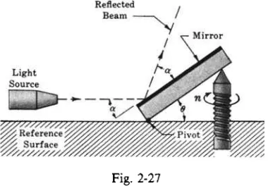
A control system is an arrangement of physical components connected or related in such a manner as to command, direct, or regulate itself or another system.

In the most abstract sense it is possible to consider every physical object a control system. Everything alters its environment in some manner, if not actively then passively-like a mirror directing a beam of light shining on it at some acute angle. The mirror (Fig. 1-1) may be considered an elementary control system, controlling the beam of light according to the simple equation “the angle of reflection a equals the angle of incidence a.”

In engineering and science we usually restrict the meaning of control systems to apply to those systems whose major function is to dynamically or actively command, direct, or regulate. The system shown in Fig. 1-2, consisting of a mirror pivoted at one end and adjusted up and down with a screw at the other end, is properly termed a control system. The angle of reflected light is regulated by means of the screw.

It is important to note, however, that control systems of interest for analysis or design purposes include not only those manufactured by humans, but those that normally exist in nature, and control systems with both manufactured and natural components.

(14)

2 INTRODUCTION [CHAP. 1

1.2 EXAMPLES OF CONTROL SYSTEMS

Control systems abound in our environment. But before exemplifying this, we define two terms: input and output, which help in identifying, delineating, or defining a control system.

Definition 1.3: The

input

is the stimulus, excitation or command applied to a control system, typically from an external energy source, usually in order to produce a specified response from the control system.

Definition

1.4: The

output

is the actual response obtained from a control system. It may or may not

be equal to the specified response implied by the input.

Inputs and outputs can have many different forms. Inputs, for example, may be physical variables, or more abstract quantities such as reference, setpoint, or desired values for the output of the control system.

The purpose of the control system usually identifies or defines the output and input. If the output and input are given, it is possible

to

identify, delineate, or define the nature of the system components. Control systems may have more than one input or output. Often all inputs and outputs are well defined by the system description. But sometimes they are not. For example, an atmospheric electrical storm may intermittently interfere with radio reception, producing an unwanted output from a loudspeaker in the form of static.

This

“noise” output

is

part of the total output as defined above, but for the purpose

of

simply identifying a system, spurious inputs producing undesirable outputs are not normally considered as inputs and outputs in the system description. However, it is usually necessary to carefully consider these extra inputs and outputs when the system is examined in detail.

The terms input and output

also

may be used in the description of any type of system, whether or not it is a control system, and a control system may be part of a larger system, in which case it is called a

subsystem

or

control subsystem,

and its inputs and outputs may then be internal variables of the larger system.

EXAMPLE 1.1.

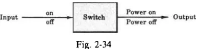
definition, the apparatus or person flipping the switch is not a part of this control system.

or off. The output is the flow or nonflow (two states) of electricity.

An

electric switch is a manufactured control system, controlling the flow of electricity. By

Flipping the switch on or off may be considered as the input. That is, the input can be in one of two states, on The electric switch is one of the most rudimentary control systems.

EXAMPLE 1.2. A thermostatically controlled heater or furnace automatically regulating the temperature of a room or enclosure is a control system. The input to this system is a reference temperature, usually specified by appropriately setting a thermostat. The output is the actual temperature of the room or enclosure.

When the thermostat detects that the output is less than the input, the furnace provides heat until the temperature of the enclosure becomes equal to the reference input. Then the furnace is automatically turned off. When the temperature falls somewhat below the reference temperature, the furnace is turned on again.

EXAMPLE 1.3. The seemingly simple act of pointing at an object with a Jinger requires a biological control system consisting chiefly of the eyes, the arm, hand and finger, and the brain. The input is the precise direction of the object (moving or not) with respect to some reference, and the output is the actual pointed direction with respect to

the same reference.

EXAMPLE 1.4. A part of the human temperature control system is the perspiration system. When the temperature of the air exterior to the skin becomes too high the sweat glands secrete heavily, inducing cooling of the skin by evaporation. Secretions are reduced when the desired cooling effect is achieved, or when the air temperature falls sufficiently.

(15)

CHAP. 11 INTRODUCTION

3

EXAMPLE 1.5. The control system consisting of a person driving an automobile has components which are clearly both manufactured and biological. The driver wants to keep the automobile in the appropriate lane of the roadway. He or she accomplishes this by constantly watching the direction of the automobile with respect to the direction of the road. In this case, the direction or heading of the road, represented by the painted guide line or lines on either side of the lane may be considered as the input. The heading of the automobile is the output of the system. The driver controls this output by constantly measuring it with his or her eyes and brain, and correcting it with his or her hands on the steering wheel. The major components of this control system are the driver’s hands, eyes and brain, and the vehicle.

1.3

OPEN-LOOP

AND

CLOSED-LOOP CONTROL SYSTEMS

Control systems are classified into two general categories:

open-loop

and

closed-loop

systems. The distinction is determined by the

control action,

that quantity responsible for activating the system to produce the output.

The term

control action

is classical in the control systems literature, but the word

action

in this expression does not always

directly

imply change, motion, or activity. For example, the control action in a system designed to have an object hit a target is usually the

distance

between the object and the target. Distance, as such, is not an action, but action (motion) is implied here, because the goal of such a control system is to reduce this distance to zero.

Definition 1.5 An

open-loop

control system is one in which the control action is independent of the output.

Definition 1.6 A

closed-loop

control system is one in which the control action is somehow dependent on the output.

Two outstanding features of open-loop control systems are:

1. Their ability to perform accurately is determined by their calibration. To

calibrate

means to establish or reestablish the input-output relation to obtain a desired system accuracy.

2. They are not usually troubled with problems

of

instability,

a concept to be subsequently discussed in detail.

Closed-loop control systems are more commonly called

feedback

control systems, and are considered in more detail beginning in the next section.

To

classify a.contro1 system as open-loop or closed-loop, we must distinguish clearly the components of the system from components that interact with but are not part of the system. For example, the driver in Example

1.5

was defined as part of that control system, but a human operator may or may not be a component of a system.

EXAMPLE 1.6. Most automatic toasters are open-loop systems because they are controlled by a timer. The time required to make ‘‘good toast” must be estimated by the user, who is not part of the system. Control over the quality of toast (the output) is removed once the time, which is both the input and the control action, has been set. The time is typically set by means of a calibrated dial or switch.

(16)

4 INTRODUCTION [CHAP. 1

1.4 FEEDBACK

Feedback is that characteristic

of

closed-loop control systems which distinguishes them from open-loop systems.

Definition 1.7: Feedback is that property of a closed-loop system which permits the output (or some other controlled variable)

to

be compared with the input to the system (or an input to some other internally situated component or subsystem) so that the appropriate control action may be formed as some function of the output and input.

More generally, feedback is said to exist in a system when a closed sequence of cause-and-effect relations exists between system variables.

EXAMPLE 1.8. The concept of feedback is clearly illustrated by the autopilot mechanism of Example 1.7. The input is the specified heading, which may be set on a dial or other instrument of the airplane control panel, and the output is the actual heading, as determined by automatic navigation instruments. A comparison device continuously monitors the input and output. When the two are in correspondence, control action is not required. When a difference exists between the input and output, the comparison device delivers a control action signal to the controller, the autopilot mechanism. The controller provides the appropriate signals to the control surfaces of the airplane to reduce the input-output difference. Feedback may be effected by mechanical or electrical connections from the navigation instruments, measuring the heading, to the comparison device. In practice, the comparison device may be integrated within the autopilot mechanism.

1.5

CHARACTERISTICS OF FEEDBACK

The presence of feedback typically imparts the following properties to a system.

1.

2.

3.

4. 5. 6.

Increased accuracy. For example, the ability to faithfully reproduce the input. This property is illustrated throughout the text.

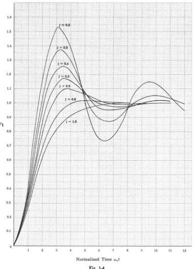
Tendency toward oscillation or instability. This all-important characteristic is considered in detail in Chapters

5

and 9 through 19.

Reduced sensitivity of the ratio of output to input to variations in system parameters and other characteristics (Chapter 9).

Reduced effects of nonlinearities (Chapters

3

and 19).

Reduced effects of external disturbances or noise (Chapters 7, 9, and 10).

Increased bandwidth. The bandwidth of a system is a frequency response measure of how well the system responds to (or filters) variations (or frequencies) in the input signal (Chapters 6, 10, 12, and 15 through 18).

1.6

ANALOG AND DIGITAL CONTROL SYSTEMS

The signals in a control system, for example, the input and the output waveforms, are typically functions of some independent variable, usually time, denoted t.

Definition 1 . 8 A signal dependent on a continuum of values of the independent variable t is called a continuous-time signal or, more generally, a continuous-data signal

or

(less fre- quently) an analog signal.

(17)

CHAP. 11 INTRODUCTION

5

We remark that

digital

is a somewhat more specialized term, particularly in other contexts. We use it as a synonym here because it is the convention in the control systems literature.

EXAMPLE 1.9. The continuous, sinusoidally varying voltage o ( t ) or alternating current i ( t ) available from an ordinary household electrical receptable is a continuous-time (analog) signal, because it is defined at each and eoery instant of time t electrical power is available from that outlet.

EXAMPLE 1.10. If a lamp is connected to the receptacle in Example 1.9, and it is switched on and then immediately off every minute, the light from the lamp is a discrete-time signal, on only for an instant every minute.

EXAMPLE 1.11. The mean temperature T in a room at precisely 8 A.M. (08 hours) each day is a discrete-time

signal. This signal may be denoted in several ways, depending on the application; for example T(8) for the temperature at 8 o’clock-rather than another time; T(l), T(2),

. . .

for the temperature at 8 o’clock on day 1, day 2, etc., or, equivalently, using a subscript notation, T,,

c,

etc. Note that these discrete-time signals are sampled values

of a continuous-time signal, the mean temperature of the room at all times, denoted T( t).

EXAMPLE 1.1 2. The signals inside digital computers and microprocessors are inherently discrete-time, or discrete-data, or digital (or digitally coded) signals. At their most basic level, they are typically in the form of sequences of voltages, currents, light intensities, or other physical variables, at either of two constant levels, for example, f 1 5 V; light-on, light-off etc. These binary signals are usually represented in alphanumeric form (numbers, letters, or other characters) at the inputs and outputs of such digital devices. On the other hand, the

signals of analog computers and other analog devices are continuous-time.

Control systems can be classified according to the types of signals they process: continuous-time (analog), discrete-time (digital), or a combination of both (hybrid).

Definition

I . 10:

Continuous-time control systems,

also called

continuous-data control systems,

or

analog control systems,

contain or process only continuous-time (analog) signals and components.

Definition

1.11:

Discrete-time control systems,

also called

discrete-data control systems,

or

sampled-

data control systems,

have discrete-time signals or components at one or more points in the system.

We note that discrete-time control systems can have continuous-time as well as discrete-time signals; that is, they can be hybrid. The distinguishing factor is that a discrete-time or digital control system

must

include at least one discrete-data signal. Also, digital control systems, particularly of sampled-data type, often have both open-loop and closed-loop modes of operation.

EXAMPLE 1.13. A target tracking and following system, such as the one described in Example 1.3 (tracking and pointing at an object with a finger), is usually considered an analog or continuous-time control system, because the distance between the “tracker” (finger) and the target is a continuous function of time, and the objective of such a Fntrol system is to continuously follow the target. The system consisting of a person driving an automobile (Example 1.5) falls in the same category. Strictly speaking, however, tracking systems, both natural and manufactured, can have digital signals or components. For example, control signals from the brain are often treated as

“pulsed” or discrete-time data in more detailed models which include the brain, and digital computers or microprocessors have replaced many analog components in vehicle control systems and tracking mechanisms.

(18)

6

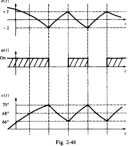
INTRODUCTION [CHAP. 1

continuous-time signal at its input, the actual room temperature, and it delivers a discrete-time (binary) switching signal at its output, turning the furnace on or off. Actual room temperature thus varies continuously between 66"

and 7OoF, and mean temperature is controlled at about 68"F, the setpoint of the thermostat.

The terms discrete-time and discrete-data, sampled-data, and continuous-time and continuous-data are often abbreviated as

discrete, sampled,

and

continuous

in the remainder of the book, wherever the meaning is unambiguous.

Digital

or

analog

is also used in place of discrete (sampled) or continuous where appropriate and when the meaning is clear from the context.

1.7

THE

CONTROL SYSTEMS ENGINEERING PROBLEM

Control systems engineering consists of

analysis

and

design

of control systems configurations.

Analysis

is the investigation

of

the properties of an existing system. The

design

problem is the Two methods exist for design:

1. Design by analysis 2. Design by synthesis

Design by analysis

is accomplished by modifying the characteristics of an existing

or

standard system configuration, and

design by synthesis

by defining the form of the system directly from its specifications.

choice and arrangement

of

system components to perform a specific task.

1.8

CONTROL SYSTEM MODELS OR REPRESENTATIONS

To

solve a control systems problem, we must put the specifications or description of the system Three basic representations (models) of components and systems are used extensively in the study configuration and its components into a form amenable to analysis or design.

of

control systems:

1.

2. Block diagrams

3.

Signal flow graphs

Mathematical models of control systems are developed in Chapters

3

and 4. Block diagrams and signal flow graphs are shorthand, graphical representations of either the schematic diagram of a system, or the set

of

mathematical equations characterizing its parts. Block diagrams are considered in detail in Chapters 2 and

7,

and signal flow graphs in Chapter

8.

Mathematical models are needed when quantitative relationships are required, for example, to represent the detailed behavior of the output of a feedback system to a given input. Development of mathematical models is usually based on principles from the physical, biological, social, or information sciences, depending on the control system application area, and the complexity of such models varies widely. One class of models, commonly called

linear systems,

has found very broad application in control system science. Techniques for solving linear system models are well established and docu- mented in the literature of applied mathematics and engineering, and the major focus of this book is linear feedback control systems, their analysis and their design. Continuous-time (continuous, analog) systems are emphasized, but discrete-time (discrete, digital) systems techniques are

also

developed throughout the text, in a unifying but not exhaustive manner. Techniques for analysis and design

of

nonlinear

control systems are the subject of Chapter 19, by way of introduction to this more complex subject

.

(19)

CHAP. 11 INTRODUCTION

7

In order to communicate with

as

many readers as possible, the material in this book is developed from basic principles in the sciences and applied mathematics, and specific applications in various engineering and other disciplines are presented in the examples and in the solved problems at the end

of

each chapter.

Solved

Problems

INPUT

AND OUTPUT

1.1. Identify the input and output for the pivoted, adjustable mirror of Fig.

1-2.

The input is the angle of inclination of the mirror 8, varied by turning the screw. The output is the angular position of the reflected beam 8

+

a from the reference surface.

1.2. Identify a possible input and a possible output for a rotational generator

of

electricity.

The input may be the rotational speed of the prime mover (e.g., a steam turbine), in revolutions per minute. Assuming the generator has no load attached to its output terminals, the output may be the induced voltage at the output terminals.

Alternatively, the input can be expressed as angular momentum of the prime mover shaft, and the output in units of electrical power (watts) with a load attached to the generator.

13. Identify the input and output for an automatic washing machine.

Many washing machines operate in the following manner. After the clothes have been put into the machine, the soap or detergent, bleach, and water are entered in the proper amounts. The wash and spin cycle-time is then set on a timer and the washer is energized. When the cycle is completed, the machine shuts itself off.

If the proper amounts of detergent, bleach, and water, and the appropriate temperature of the water are predetermined or specified by the machine manufacturer, or automatically entered by the machine itself, then the input is the time (in minutes) for the wash and spin cycle. The timer is usually set by a human operator.

The output of a washing machine is more difficult to identify. Let us define clean as the absence of foreign substances from the items to be washed. Then we can identdy the output as the percentage of cleanliness. At the start of a cycle the output is less than 100%, and at the end of a cycle the output is ideally equal to 100% (clean clothes are not always obtained).

For most coin-operated machines the cycle-time is preset, and the machine begins operating when the

coin is entered. In this case, the percentage of cleanliness can be controlled by adjusting the amounts of

detergent, bleach, water, and the temperature of the water. We may consider all of these quantities as

inputs.

Other combinations of inputs and outputs are also possible.

1.4. Identify the organ-system components, and the input and output, and describe the operation of the biological control system consisting of a human being reaching for

an

object.

The basic components of this intentionally oversimplified control system description are the brain, arm and hand, and eyes.

The brain sends the required nervous system signal to the arm and hand to reach for the object. This signal is amplified in the muscles of the arm and hand, which serve as power actuators for the system. The eyes are employed as a sensing device, continuously “feeding back” the position of the hand to the brain.

(20)

8

INTRODUCTION [CHAP. 1

The objective of the control system is to reduce the distance between hand position and object position to zero. Figure 1-3 is a schematic diagram. The dashed lines and arrows represent the direction of information flow.

OPEN-LOOP AND CLOSED-LOOP SYSTEMS

1.5. Explain how a closed-loop automatic washing machine might operate.

Assume all quantities described as possible inputs in Problem 1.3, namely cycle-time, water volume, water temperature, amount of detergent, and amount of bleach, can be adjusted by devices such as valves and heaters.

A closed-loop automatic washer might continuously or periodically measure the percentage of cleanliness (output) of the items being washing, adjust the input quantities accordingly, and turn itself off when 100% cleanliness has been achieved.

1.6. How are the following open-loop systems calibrated: ( a ) automatic washing machine, ( b ) automatic toaster, ( c ) voltmeter?

Automatic washing machines are calibrated by estimating any combination of the following input quantities: (1) amount of detergent, (2) amount of bleach or other additives, (3) amount of water, (4) temperature of the water, ( 5 ) cycle-time.

On some washing machines one or more of these inputs is (are) predetermined. The remaining quantities must be estimated by the user and depend upon factors such as degree of hardness of the water, type of detergent, and type or strength of the bleach or other additives. Once this calibration has been determined for a specific type of wash (e.g., all white clothes, very dirty clothes), it does not normally have to be redetermined during the lifetime of the machine. If the machine breaks down and replacement parts are installed, recalibration may be necessary.

Although the timer dial for most automatic toasters is calibrated by the manufacturer (e.g., light- medium-dark), the amount of heat produced by the heating element may vary over a wide range. In addition, the efficiency of the heating element normally deteriorates

with

age. Hence the amount of time required for “good toast” must be estimated by the user, and this setting usually must be periodically readjusted. At first, the toast is usually too light or too dark. After several successively different estimates, the required toasting time for a desired quality of toast is obtained.

In general, a voltmeter is calibrated by comparing it with a known-voltage standard source, and appropriately marking the reading scale at specified intervals.

1.7. Identify the control action in the systems of Problems 1.1,

1.2,

and

1.4.

For the mirror system of Problem 1.1 the control action is equal to the input, that is, the angle of

rotational speed or angular momentum of the prime mover shaft. The control action of the human reaching

Mathcad inclination of the mirror 6 . For the generator of Problem 1.2 the control action is equal to the input, the

(21)

CHAP. 11

INTRODUCTION

9

1.8.

Mathcad

a

1.9.

1.10.

Which of the control systems in Problems 1.1, 1.2, and 1.4 are open-loop? Closed-loop?

Since the control action is equal to the input for the systems of Problems 1.1 and 1.2, no feedback exists and the systems are open-loop. The human reaching system of Problem 1.4 is closed-loop because the control action is dependent upon the output, hand position.

Identify the control action in Examples

1.1

through 1.5.

The control action for the electric switch of Example 1.1 is equal to the input, the on or off command. The control action for the heating system of Example 1.2 is equal to the difference between the reference and actual room temperatures. For the finger pointing system of Example 1.3, the control action is equal to the difference between the actual and pointed direction of the object. The perspiration system of Example 1.4 has its control action equal to the difference between the "normal" and actual skin surface temperature. The difference between the direction of the road and the heading of the automobile is the control action for the human driver and automobile system of Example 1.5.

Which of the control systems in Examples 1.1 through 1.5 are open-loop? Closed-loop?

The electric switch of Example 1.1 is open-loop because the control action is equal to the input, and therefore independent of the output. For the remaining Examples 1.2 through 1.5 the control action is clearly a function of the output. Hence they are closed-loop systems.

FEEDBACK

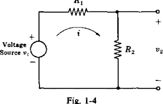
1.11. Consider the voltage divider network of Fig. 1-4. The output is U, and the input is ul.

Fig. 1-4

( a ) Write an equation for u2 as a function of U,,

R,,

and

R,.

That is, write an equation for u2

which yields an open-loop system.

( b ) Write an equation for U, in closed-loop

form,

that is, u2 as a function of U,, U,,

R,,

and

This problem illustrates how a passive network can be characterized as either

an

open-loop

R 2 .

or a closed-loop system.

( a ) From Ohm's law and Kirchhoffs voltage and current laws we have

U 1

U, = R2i i=-

Rl + R 2

Therefore

[image:21.567.202.367.360.466.2]

(22)

10 INTRODUCTION [CHAP. 1

1.12. Explain how the classical economic concept known as the Law of Supply and Demand can be interpreted as a feedback control system. Choose the market price (selling price) of a particular item as the output of the system, and assume the objective of the system is to maintain price stability.

The Law can be stated in the following manner. The market demand for the item decreases as its price increases. The market supply usually increases as its price increases. The Law of Supply and Demand says that a stable market price is achieved if and only if the supply is equal to the demand.

The manner in which the price is regulated by the supply and the demand can be described with feedback control concepts. Let us choose the following four basic elements for our system: the Supplier, the Demander, the Pricer, and the Market where the item is bought and sold. (In reality, these elements generally represent very complicated processes.)

The input to our idealized economic system is price stability the “desired” output. A more convenient way to describe this input is zeropricefluctuation. The output is the actual market price.

The system operates as follows: The Pricer receives a command (zero) for price stability. It estimates a price for the Market transaction with the help of information from its memory or records of past transactions. This price causes the Supplier to produce or supply a certain number of items, and the Demander to demand a number of items. The difference between the supply and the demand is the control action for this system. If the control action is nonzero, that is, if the supply is not equal to the demand, the Pricer initiates a change in the market price in a direction which makes the supply eventually equal to the demand. Hence both the Supplier and the Demander may be considered the feedback, since they determine the control action.

MISCELLANEOUS PROBLEMS

1.13. ( a ) Explain the operation of ordinary traffic signals whrch control automobile traffic at roadway intersections. ( b ) Why are they open-loop control systems? ( c ) How can traffic be controlled more efficiently? ( d ) Why is the system of (c) closed-loop?

( a ) Traffic lights control the flow of traffic by successively confronting the traffic in a particular direction (e.g., north-south) with a red (stop) and then a green (go) light. When one direction has the green signal, the cross traffic in the other direction (east-west) has the red. Most traffic signal red and green light intervals are predetermined by a calibrated timing mechanism.

Control systems operated by preset timing mechanisms are open-loop. The control action is equal to the input, the red and green intervals.

Besides preventing collisions, it is a function of traffic signals to generally control the volume of traffic. For the open-loop system described above, the volume of traffic does not influence the preset red and green timing intervals. In order to make traffic flow more smoothly, the green light timing interval must be made longer than the red in the direction containing the greater traffic volume. Often a traffic officer performs this task.

The ideal system would automatically measure the volume of traffic in all directions, using appropriate sensing devices, compare them, and use the difference to control the red and green time intervals, an ideal task for a computer.

( d ) The system of ( c ) is closed-loop because the control action (the difference between the volume of traffic in each direction) is a function of the output (actual traffic volume flowing past the intersection in each direction).

( b )

( c )

1.14. ( a ) Describe, in a simplified way, the components and variables of the biological control system involved in walking in a prescribed direction. ( b ) Why is walking a closed-loop operation? (c) Under what conditions would the human walking apparatus become an open-loop system? A sampled-data system? Assume the person has normal vision.

( a ) The major components involved in walking are the brain, eyes, and legs and feet. The input may be chosen as the desired walk direction, and the output the actual walk direction. The control action is determined by the eyes, which detect the difference between the input and output and send this information to the brain. The brain commands the legs and feet to walk in the prescribed direction. Walking is a closed-loop operation because the control action is a function of the output.

(23)

CHAP. 13 INTRODUCTION 11

( c ) If the eyes are closed, the feedback loop is broken and the system becomes open-loop. If the eyes are

opened and closed periodically, the system becomes a sampled-data one, and wallung is usually more accurately controlled than with the eyes always closed.

1.15. Devise a control system to fill a container with water after it is emptied through a stopcock at the bottom. The system must automatically shut off the water when the container is filled.

The simplified schematic diagram (Fig. 1-5) illustrates the principle of the ordinary toilet tank filling system.

The ball floats on the water. As the ball gets closer to the top of the container, the stopper decreases the flow of water. When the container becomes full, the stopper shuts off the flow of water.

1.16. Devise a simple control system which automatically turns on a room lamp at dusk, and turns it off in daylight.

A simple system that accomplishes t h s task is shown in Fig. 1-6.

At dusk, the photocell, which functions as a light-sensitive switch, closes the lamp circuit, thereby lighting the room. The lamp stays lighted until daylight, at which time the photocell detects the bright outdoor light and opens the lamp circuit.

1.17. Devise a closed-loop automatic toaster.

(24)

12 INTRODUCTION [CHAP. 1

The toaster is initially calibrated for a desired toast quality by means of the color adjustment knob. T h ~ s setting never needs readjustment unless the toast quality criterion changes. When the switch is closed, the bread is toasted until the color detector “sees” the desired color. Then the switch is automatically opened by means of the feedback linkage, which may be electrical or mechanical.

1.18. Is the voltage divider network in Problem 1.11 an analog or digital device? Also, are the input and output analog or digital signals?

It is clearly an analog device, as are all electrical networks consisting only of passive elements such as

resistors, capacitors, and inductors. The voltage source u1 is considered an external input to this network. If it produces a continuous signal, for example, from a battery or alternating power source, the output is a continuous or analog signal. However, if the voltage source u1 is a discrete-time or digital signal, then so is the output U? = u1 R 2 / (

R,

+

R 2 ) . Also, if a switch were included in the circuit, in series with an analog voltage source, intermittent opening and closing of the switch would generate a sampled waveform of the voltage source and therefore a sampled or discrete-time output from t h s analog network.

1.19. Is the system that controls the total cash value of a bank account a continuous or a discrete-time system? Why? Assume a deposit is made only once, and no withdrawals are made.

If the bank pays no interest and extracts no fees for maintaining the account (like putting your money “under the mattress”), the system controlling the total cash value of the account can be considered continuous, because the value is always the same. Most banks, however, pay interest periodically, for example, daily, monthly, or yearly, and the value of the account therefore changes periodically, at discrete times. In t h s case, the system controlling the cash value of the account is a discrete system. Assuming no withdrawals, the interest is added to the principle each time the account earns interest, called compounding, and the account value continues to grow without bound (the “greatest invention of mankind,” a comment attributed to Einstein).

1.20. What type of control system, open-loop or closed-loop, continuous or discrete, is used by an ordinary stock market investor, whose objective is to profit from his or her investment.

Stock market investors typically follow the progress of their stocks, for example, their prices, periodically. They might check the bid and ask prices daily, with their broker or the daily newspaper, or more or less often, depending upon individual circumstances. In any case, they periodically sample the pricing signals and therefore the system is sampled-data, or discrete-time. However, stock prices normally rise and fall between sampling times and therefore the system operates open-loop during these periods. The feedback loop is closed only when the investor makes his or her periodic observations and acts upon the information received, which may be to buy, sell, or do nothmg. Thus overall control is closed-loop. The measurement (sampling) process could, of course, be handled more efficiently using a computer, which also can be programed to make decisions based on the information it receives. In this case the control system remains discrete-time, but not only because there is a digital computer in the control loop. Bid and ask prices do not change continuously but are inherently discrete- time signals.

Supplementary Problems

1.21. Identify the input and output for an automatic temperature-regulating oven.

1.22. Identify the input and output for an automatic refrigerator.

(25)

CHAP. 11

INTRODUCTION

13

1.24.

1.25.

1.26.

1.27.

1.28.

1.29.

130.

131.

132.

133.

134.

135.

Devise a control system to automatically raise and lower a lift-bridge to permit ships to pass. No continuous human operator is permissible. The system must function entirely automatically.

Explain the operation and identify the pertinent quantities and components of an automatic, radar-controlled antiaircraft gun. Assume that no operator is required except to initially put the system into an operational mode.

How can the electrical network of Fig. 1-8 be given a feedback control system interpretation? Is this system analog or digital?

t r 0

Fig. 1-8

Devise a control system for positioning the rudder of a ship from a control room located far from the rudder. The objective of the control system is to steer the ship in a desired heading.

What inputs in addition to the command for a desired heading would you expect to find acting on the system of Problem 1.27?

Can the application of “laissez faire capitalism” to an economic system be interpreted as a feedback control system? Why? How about “socialism” in its purest form? Why?

Does the operation of a stock exchange, for example, buying and selling equities, fit the model of the Law

of Supply and Demand described in Problem 1.12? How?

Does a purely socialistic economic system fit the model of the Law of Supply and Demand described in

Problem 1.12? Why (or why not)?

Which control systems in Problems 1.1 through 1.4 and 1.12 through 1.17 are digital or sampled-data and which are continuous or analog? Define the continuous signals and the discrete signals in each system.

Explain why economic control systems based on data obtained from typical accounting procedures are sampled-data control systems? Are they open-loop or closed-loop?

Is a rotating antenna radar system, which normally receives range and directional data once each revolution, an analog or a digital system?

(26)

14 INTRODUCTION [CHAP. 1

Answers to

Some

Supplementary Problems

1.21. The input is the reference temperature. The output is the actual oven temperature. 1.22. The input is the reference temperature. The output is the actual refrigerator temperature.

(27)

Chapter

2

Control Systems Terminology

2.1 BLOCK DIAGRAMS: FUNDAMENTALS

A

block

diagram is a shorthand, pictorial representation of the cause-and-effect relationship between the input and output of a physical system. It provides a convenient and useful method for characterizing the ‘functional relationships among the various components of a control system. System components are alternatively called elements of the system. The simplest form of the block diagram is the single block, with one input and one output, as shown in Fig.

2-1.

The interior of the rectangle representing the block usually contains a description of or the name of the element, or the symbol for the mathematical operation to be performed on the input to yield the output. The arrows represent the direction of information or signal flow.

EXAMPLE 2.1

The operations of addition and subtraction have a special representation. The block becomes a small circle, called a summing point, with the appropriate plus

or

minus sign associated with the arrows entering the circle. The output is the algebraic sum of the inputs. Any number of inputs may enter a summing point.

EXAMPLE 2.2

Fig. 2-3

(28)

16 CONTROL SYSTEMS TERMINOLOGY [CHAP. 2

Some authors put a cross in the circle: (Fig.

2-4)

Fig. 2-4

This notation is avoided here because it is sometimes confused with the multiplication operation. In order to have the same signal or variable be an input to more than one block or summing point, a

takeoff

point is used. This permits the signal to proceed unaltered along several different paths to several destinations.

EXAMPLE 2.3

t x

Takeoff Point

* x

-

(a) x

Takeoff Point

Fig. 2-5

2.2 BLOCK DIAGRAMS OF CONTINUOUS (ANALOG) FEEDBACK CONTROL SYSTEMS

The blocks representing the various components of a control system are connected in a fashion which characterizes their functional relationships within the system. The basic configuration of a simple closed-loop (feedback) control system with a single input and a single output (abbreviated

SISO)

is illustrated in Fig. 2-6 for a system with continuous signals only.

Fig. 2-6

(29)

CHAP. 21 CONTROL SYSTEMS TERMINOLOGY

17

1.2 is often chemical, from burning fuel oil, coal, or gas. But this energy source would not appear in the closed control loop of the system.

2.3

TERMINOLOGY

OF THE CLOSED-LOOP BLOCK DIAGRAM

It is important that the terms used in the closed-loop block diagram be clearly understood. Lowercase letters are used to represent the input and output variables of each element as well as the symbols for the blocks g,, g,, and

h .

These quantities represent functions of time, unless otherwise specified.

EXAMPLE 2.4. r = r( t )

In subsequent chapters, we use capital letters to denote Laplace transformed or z-transformed quantities, as functions of the complex variable s, or z , respectively, or Fourier transformed quantities (frequency functions), as functions of the pure imaginary variable j w . Functions of s or

z

are often abbreviated to the capital letter appearing alone. Frequency functions are never abbreviated.

EXAMPLE 2.5. R ( s ) may be abbreviated as R , or F ( z ) as F. R(jo) is never abbreviated.

The letters r , c, e, etc., were chosen to preserve the generic nature

of

the block diagram. This convention is now classical.

Definition 2. I :

Definition 2 . 2

Definition 2.3:

Definition 2.4

Definition

2.5

Definition 2.7:

The

plant

(or

process,

or

controlled system)

g 2 is the system, subsystem, process, or object controlled by the feedback control system.

The

controlled output

c is the output variable of the plant, under the control of the feedback control system.

The

forward path

is the transmission path from the summing point to the controlled output c.

The

feedforward (control) elements

g, are the components of the forward path that generate the control signal U or m applied to the plant. Note: Feedforward elements

typically include controller(s), compensator( s) (or equalization elements), and/or amplifiers.

The

control

signal U (or

manipulated variable

rn) is the output signal of the

feedforward elements g, applied as input to the plant g,.

The

feedback path

is the transmission path from the controlled output c back to the summing point.

The

feedback elements

h establish the functional relationship between the controlled output c and the primary feedback signal

b.

Note: Feedback elements typically include sensors of the controlled output c, compensators, and/or controller element s.

(30)

18

Decfinition 2.9:

Defiition 2.10:

Defiition 2.11:

CONTROL SYSTEMS TERMINOLOGY [CHAP. 2

The primary feedback signal b is a function of the controlled output c, algebraically summed with the reference input r to obtain the actuating (error) signal

e ,

that is, r f b = e. Note: An open-loop system has no primary feedback signal.

The actuating (or error) signal is the reference input signal r plus or minus the primary feedback signal b. The control action is generated by the actuating (error) signal in a feedback control system (see Definitions 1.5 and 1.6). Note: In an open-loop system, which has no feedback, the actuating signal is equal to r .

Negative feedback means the summing point is a subtractor, that is, e = r - b.

Positive feedback means the summing point is an adder, that is, e = r

+

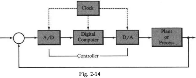
b.

2.4 BLOCK DIAGRAMS OF DISCRETE-TIME (SAMPLED-DATA, DIGITAL) COMPONENTS,

CONTROL SYSTEMS, AND COMPUTER-CONTROLLED SYSTEMS

A discrete-time (sampled-data or digital) control system was defined in Definition 1.11 as one having discrete-time signals or components at one or more points in the system. We introduce several common discrete-time system components first, and then illustrate some of the ways they are interconnected in digital control systems. We remind the reader here that discrete-time is often abbreviated as discrete in this book, and continuous-time as continuous, wherever the meaning is unambiguous.

EXAMPLE 2.6. A digital computer or microprocessor is a discrete-time (discrete or digital) device, a common component in digital control systems. The internal and external signals of a digital computer are typically discrete-time or digitally coded.

EXAMPLE 2.7. A discrete system component (or components) with discrete-time input U( t , ) and discrete-time

output y ( t k ) signals, where t, are discrete instants of t