Efficient encoding and decoding of binaural sound with resonance audio

Conference

Paper

68

Presented

at

the

Conference

on

Immersive

and

Interactive

Audio

2019

March

27

–

29,

York,

UK

Thispaperwaspeer-reviewedasacompletemanuscriptforpresentationatthisconference.ThispaperisavailableintheAES E-Library(http://www.aes.org/e-lib)allrightsreserved. Reproductionofthispaper,oranyportionthereof,isnotpermitted withoutdirectpermissionfromtheJournaloftheAudioEngineeringSociety.

Efficient Encoding and Decoding of Binaural Sound with

Resonance Audio

Marcin Gorzel1_{, Andrew Allen}1_{, Ian Kelly}1_{, Julius Kammerl}1_{, Alper Gungormusler}1_{, Hengchin Yeh}1_{, and Francis}

Boland1,2

1_{Google Inc.}

2_{Trinity College Dublin}

Correspondence should be addressed to Marcin Gorzel ([email protected])

ABSTRACT

Resonance Audio is an open source project designed for creating and controlling dynamic spatial sound in Virtual & Augmented Reality (VR/AR), gaming or video experiences. It also provides integrations with popular game development platforms and digital audio workstations (as a preview plugin). Resonance Audio binaural decoder is used in YouTube to provide binaural rendering of 360/VR videos. This paper describes the core sound spatialization algorithms used in Resonance Audio and can be treated as a companion to the Resonance Audio C++ /MATLAB

librarysource code.

1

Introduction

Resonance Audio is an open source project which al-lows developers to create and control complex virtual auditory environments in real-time. The Resonance Au-dio Software Development Kit (SDK) consists of the C++ library,MATLABlibrary of helper Digital Signal Processing (DSP) functions and also platform integra-tions which allow for immediate use of Resonance Audio within game engines and audio / video editing software. It supports all major platforms (Android, iOS, Windows, MacOS, Linux) and addresses a range of re-quirements for efficient high quality audio rendering, especially on mobile platforms, such as: thread-safety, non-blocking APIs (critical in VR/AR to ensure high frame rate and maximum CPU utilization), minimum audio processing latency (no buffered processing of audio data, single-threaded audio processing pipeline)

and a small binary footprint.

Resonance Audio users can create virtual sound sources to be rendered in a virtual 3D space with a fine control over sources’ directivity patterns, occlusion or near-field settings. They can also simulate specific acoustic environments via early reflections and late reverbera-tion.

The “spatializer" is the core concept of the Resonance Audio system which encapsulates algorithms responsi-ble for efficient encoding of sound events into an inter-mediate format - Ambisonics [1,2], manipulation and, finally, binaural decoding of Ambisonic soundfields.

at a constant storage and computational cost with an arbitrary level of spatial accuracy, as will be explained in more detail in Section1.2. This representation is used to render an approximation of the original sound-field using either loudspeakers or headphones. The decoding part only is used in cinematic 360/VR video experiences (like YouTube 360/VR) where the spatial audio content is streamed along with the video content.

This paper describes the core algorithms used in the Resonance Audio’s spatializer. It is organized as fol-lows: The reminder of this section explains the con-ventions used in this paper and provides background information about encoding, decoding and binaural re-production of spatial audio using Ambisonics. Section 1.2.1describes a novel method of efficient encoding of sound sources into Ambisonic soundfield representa-tion. It also talks about controlling the angular spread of sound sources. Section3describes an optimized method of binaural decoding of Ambisonic soundfields based on pre-computed, spherical harmonic-encoded binaural filters. Finally, Section4summarizes the pa-per and suggest some future research and development directions.

1.1 Conventions Used in Resonance Audio

1.1.1 3D Coordinate System

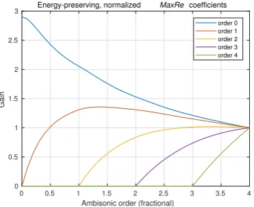
The 3D coordinate system used in this paper is pre-sented in Figure1. It usesx,yandzaxes pointing to the front, left and up respectively.φis the azimuth angle with an anti-clockwise rotation andθis the elevation angle calculated from the x-y plane. The conversion between spherical and Cartesian coordinates is defined as:

x = k~rkcos(φ)cos(θ) y = k~rksin(φ)cos(θ) z = k~rksin(θ)

(1)

1.1.2 Ambisonic Channel Sequence and Normalization

Resonance Audio uses the AmbiX Ambisonic conven-tion for encoding and decoding of sound objects, as defined in [4]. It uses Schmidt semi-normalized har-monics (SN3D normalization) and Ambisonic Chan-nel Number (ACN) sequencing of spherical harmonics (SHs) - the basis functions used in Ambisonics.

roll

yaw

pitch

x

y z

r

θ 0

φ

Fig. 1:3D spherical coordinate system used in this

paper, as proposed in [3]

1.1.3 Other Conventions

Traditional maths and physics use the terms degree

(usually denoted asl) andorder(usually denoted as

m) where 0≤l≤+∞and−m≤l ≤mto describe SHs. In contrast, inFirst Order Ambisonics(FOA) orHigher Order Ambisonics(HOA), the termsorder

(usually denoted asn) anddegree(usually denoted as

m) are used in the opposite meaning [4].

The Resonance Audio source code, whenever we are concerned with spherical harmonics directly, uses the traditional naming convention (for example a spherical harmonic of degreeland order−m≤l≤m).

However, when it is more natural to use the Ambisonic convention, we use the wordAmbisonicexplicitly, for exampleAmbisonic orderand (less often)Ambisonic degree.

To obtain the ACN from a given Ambisonic order and degree, one has to do the following:

ACN=n2+n+m (2)

Conversely, to retrieve the Ambisonic order and degree information from a given Ambisonic channel in an ACN sequence:

n=b√ACNc (3)

m=ACN−n2−n (4)

1.2 Higher Order Ambisonic Soundfields

1.2.1 Encoding Ambisonics

To encode a sound source into an Ambisonic soundfield, we take an outer product of the monophonic pressure signal corresponding to the sound source,s, and the vectoryof SH coefficientsYm

n(φ,θ):

B=s⊗y (5)

Spherical harmonic coefficients are defined as:

Y_nm(φ,θ) =Nn|m|P |m|

n (sin(θ))

cos(|m|φ) ifm≥0 sin(|m|φ) ifm<0 (6)

whereφis the source horizontal angle,θis the source vertical angle,nis the Ambisonic order,mis the Am-bisonic degree1_,P|m|

n are the associated Legendre

func-tions (with the Condon-Shortley phaseundone).Nn|m|

is the SN3D normalization term which is computed according to the following formula:

Nn|m|= s

(2−δm)

(n− |m|)!

(n+|m|)! (7)

Note that we skip the ₄1

π term in the normalization

which means that we are preserving the original source amplitude in the 0thorder Ambisonic channel.

1.2.2 Ambisonic Transformations

An arbitrary Ambisonic transformation can be de-scribed as:

e

B=BT (8)

where the new, transformed Ambisonic signalBeis

ob-tained by applying a matrixTto the Ambisonic input signalB.

There are different types of transformations that can be applied to an Ambisonic soundfield [5]. For example, rotation can be applied to a single soundfield which can consist of multiple point sources. Another transforma-tion used in Resonance Audio which is applied on a

1_{Please see Section1.1.3for explanation of the conventions used.}

per-sound source basis is angular spread control (see Section2.2).

Sound sources encoded into an Ambisonic represen-tation are assumed to be dynamic, i.e. their position relative to the listener’s head can change at an arbi-trary rate and independently of the other sound sources. Hence, to re-position an individual sound source in the 3D space it suffices to re-encode it with updated SH coefficients.

There are situations, however, where rotating an Am-bisonic soundfield is a better solution. One such sit-uation is when multiple sound sources are used and when the sources have already been encoded into the Ambisonic representation, for example, using a micro-phone array.

FOA rotation is trivial and consists in applying a 3 x 3 rotation matrix to the velocity components of the soundfield whereas keeping the pressure component un-modified. This is equivalent to a simple vector rotation inR3. In Resonance Audio, this transformation is

ap-plied by theFoaRotatorNodewith the underlying DSP implemented by theFoaRotatorclass.

HOA rotation is more complex since it requires rota-tions of vectors whose dimensionality is higher than 3. Numerous methods have been proposed to com-pute the required rotation matrices in_R4 _{and above,}

for example in [5]. Resonance Audio uses an effi-cient computation of SH rotation matrices by recursion, used in other fields like physical chemistry or com-puter graphics [6,7,8]. HOA rotation is applied by the

HoaRotatorNodewith the underlying DSP imple-mented by theHoaRotatorclass.

1.2.3 Decoding Ambisonics

The decoding of an Ambisonic signal Bis done by multiplying it with the inverse of the loudspeaker re-encodingmatrixLwhich encodes each loudspeaker’s direction into SHs:

L=



   

Y₀0(Φ1,Θ1) Y00(Φi,Θi) . . . Y00(ΦN,ΘN)

Y₁−1(Φ1,Θ1) Y₁−1(Φi,Θi) . . . Y₁−1(ΦN,ΘN)

..

. ... ... ...

Ym

n(Φ1,Θ1) Ynm(Φi,Θi) . . . Ynm(ΦN,ΘN) 

   

whereΦiandΘiare azimuth and vertical angles of the

ithloudspeaker in the array. The resultant loudspeaker signalsGare obtained by:

G=BD (10)

whereDis a Moore-Penrose pseudo-inverse ofL:

D=L†=LT(LLT)−1 (11)

1.2.4 Frequency-dependent Decoder Optimization

In Ambisonics, the area of correct soundfield recon-struction is located around the so-called “sweet-spot". The size of this area depends on the frequency con-tent of the soundfield and the Ambisonic order of a system. For example, Danielet al.in [3] and [9] eval-uated soundfield reconstruction errors for Ambisonic orders of 1 to 5 and proposed cut-off frequencies below which the Ambisonic reconstruction can be considered as accurate.

Gerzon proposed objective criteria for good localiza-tion in multi-loudspeaker systems in [10,11] by eval-uating velocity and energy vectors characterizing the soundfield. For example, low frequency localization for humans is mainly based on the interaural phase differences. On the other hand, in the mid- and high-frequency range, interaural level differences start to play a much greater role in localization. That is why, Gerzon suggested to optimize the velocity vectors at low frequencies and the energy vectors at mid- and high frequencies.

One way to apply these optimizations in Ambisonic playback is to use different decoder types in their most optimal frequency bands. Decoders that utilize differ-ent decoding schemes in differdiffer-ent frequency ranges are known as shelf-filter decoders or dual-band decoders [12,13,14]. In such decoders, phase-matched shelf-filters are typically used to split the Ambisonic signal spectrum into low- and mid/high-frequency bands. The cross-over frequency of the filters is usually set so that thebasic decoder operates only at low frequencies, where the soundfield reconstruction errors do not ex-ist or are minimal. This decoder already maximizes the lengths of velocity vectors. Above the crossover frequency, a different decoding scheme is used which maximizes the lengths of energy vectors and thus, the

energy concentration in the direction of an encoded sound source. This is known as the maximum-energy orMaxRedecoder.

Different decoding schemes are applied by changing the ratios of the pressure and velocity soundfield com-ponents at different Ambisonic orders. The closed-form closed-formulae for obtaining (MaxRe) decoder coeffi-cients (as well as other decoder types) have been given, for example, by Daniel in [3].

Resonance Audio implements dual-band decoders where cut-off frequencies are based on the soundfield reconstruction errors proposed by Daniel in [3]. The cross-over frequencies at Ambisonic orders 1 to 5 are set to the following values: 690Hz, 1250Hz, 1831Hz, 2423Hz, 3022Hz. These values can be modified by changing the ambishelffilter MATLAB func-tion and re-generating the binaural Ambisonic decoders. The binaural Ambisonic decoders in Resonance Audio are pre-emphasized using shelf-filters which greatly reduces computational load at run-time (please see Sec-tion3for more details).

1.3 Binaural Reproduction of Ambisonic Soundfields

Binaural reproduction of Ambisonic soundfields is typ-ically done using “virtual loudspeakers". This method was first introduced by McKeag and McGrath [15] and examples of its adoption can be found in work by Nois-terniget al.[16] or Dalenbacket al.[17].

In this method, loudspeaker signals are first generated by decoding an Ambisonic soundfield. Next, they are convolved with the Head Related Impulse Responses (HRIRs) corresponding to the physical loudspeaker locations. Lastly, left channel signals are summed to-gether to create the left feed of a binaural signal. The same process is repeated for the right feed. For exam-ple, to obtain the left and right ear headphone signals

plandprwe have to perform:

pl=

N

∑

i=1

hLi∗gi (12)

pr= N

∑

i=1

HRIR measurement

(a)

Binaural Playback Virtual source

(b)

Fig. 2:The “virtual loudspeakers" reproduction con-cept: (a) measurement of HRIRs corresponding to the spatial locations of all the loudspeakers required by the decoder; (b) two or more loud-speaker signals are convolved with the corre-sponding HRIRs and summed together, form-ing a 2-channel binaural output

where hLi and hRi HRIRs for the left and right ear

respectively, corresponding to theith_loudspeaker

loca-tion;giis theithloudspeaker signal and∗denotes the

convolution process2.

In the “virtual loudspeakers" approach, HRIRs are mea-sured at the “sweet spot" and then selected measure-ments are used by the decoder. Resonance Audio uses measurements provided in the open sourceSADIE Bin-aural Measurementsdatabase [18]. Decoder config-urations used for Ambisonic orders 1 to 5 are: Cube, Dodecahedron, 26-point Lebedev grid, Pentakis Dodec-ahedron and Pentakis IcosidodecDodec-ahedron respectively. The concept of forming the “virtual loudspeakers" from an array of loudspeakers is illustrated in Figure2.

The number of convolutions necessary in the “virtual loudspeakers" method is equal to twice the number of loudspeakers used in the Ambisonic decoder. For ex-ample, for the 1st order cube decoder, 16 convolutions would be used; for the 3rdorder Lebedev grid decoder, 52 convolutions would be used, etc. In practice, Res-onance Audio uses several optimizations that signifi-cantly reduce the number of convolutions required and thus minimizes the computational load at run-time. For more information, please see Section3.

2_{Please note that HRIR convolution in the time domain is}

equiv-alent with the HRTF multiplication in the frequency domain. We use HRIR convolution in the below examples although it is implied that these operations are performed more efficiently in the frequency domain.

2

Efficient Encoding of Sound Sources

Real-time computation of SH coefficients is CPU in-tensive, as can be inferred from Equations6and 7. Ideally, the SH coefficients would be pre-computed and stored in a Look Up Table (LUT) to minimize run-time complexity while keeping the memory footprint and pre-computation initialization time at a minimum.

Resonance Audio uses a novel method which exploits symmetries of SH functions to efficiently pre-compute, index and store and then retrieve the coefficients at run-time. This allows a reduction of the memory footprint and pre-computation speed up of∼8x.

2.1 Exploiting Symmetries of Spherical Harmonics

SH functions can be symmetric against x, y and/or z Cartesian axes. For example:

Y_nm(φ,θ) =Y_nm(−φ,θ) (14)

indicates thatYm

n(φ,θ)is symmetric with respect to the

sagittal plane (i.e. left-right symmetry) but at the same time is anti-symmetric with respect to the horizontal plane (e.g. up-down anti-symmetry):

Y_nm(φ,θ) =−Y_nm(φ,−θ) (15)

An SH which exhibits the above properties is, for ex-ample,Y₁0(φ,θ)(ACN=2):

Fig. 3:Front-back symmetric / left-right symmetric /

up-down anti-symmetric SH functionY₁0(φ,θ)

It is also possible that an SH is left-right and up-down symmetric, but front-back anti-symmetric, for example:

Y_nm(φ,θ) =−Y_nm(φ,−θ) (16)

Fig. 4:Front-back symmetric / left-right anti-symmetric / up-down anti-symmetric SH function

Y3 3(φ,θ)

In general, and without a formal proof, symmetry/anti-symmetry-related sign flip for a given SHY_nm(φ,θ) with respect to they,z, andxaxis can be written as:

ξy(n,m) =

1 ifm≥0

−1 ifm<0 (17)

ξz(n,m) = (−1)n+m (18)

ξx(n,m) =

(−1)m ifm≥0

−(−1)|m| ifm<0 (19)

whereξ is a symmetry-related phase coefficient for the relevant axis. Therefore, if we pre-compute and store only one sphere quadrant of the SH coefficients, we can utilize the above symmetry information to retrieve an arbitrary SH coefficient of the same order and degree. Whether to employ a given phase coefficient depends on which quadrant we decide to pre-compute as well as which quadrant the sound source is located in. For example, with the pre-computed front-left-top quadrant (0≤φ≤π₂, 0≤θ≤π₂) to retrieve an SH coefficient for an arbitrary angle pair in the rear-right-bottom quadrant (−π≤φ≤ −π₂,−π₂≤θ≤0) we can do:

Y_nm(φ,θ) =ξy(n,m)ξz(n,m)ξx(n,m)Ynm(π− |φ|,|θ|)

(20)

Similar logic can be applied to find the SH coeffi-cients for other sound source directions (i.e. in other sphere quadrants), by simply dropping the redundant symmetry-related phase coefficients and constraining the angle look-up to the[0,π

2]range.

In Resonance Audio, AmbisonicLookupTable

implements the above method for fast retrieval of SH coefficients. It first computes a limited size LUT of SH coefficients for angles in the[0,π

2]range

at 1◦ resolution (ComputeEncoderTable,

as well as the symmetry information LUT

ComputeSymmetriesTable on system start-up. Then, at run-time, the SH encoding coef-ficients can be rapidly retrieved by calling the

GetEncodingCoeffsmethod.

Similarly, MATLAB users can

uti-lize the described algorithm by using

getencodertable, getshsymmetries

and ambencodecoeffsymmetric functions respectively.

Apart from fast encoding of the sound source direction, Resonance Audio also allows to efficiently model its angular spread, which has multiple uses in sound design (for example, to simulate sound source width or create volumetric sound sources). This will be described in more detail in the next section.

2.2 Controlling Sound Source Spread

Angular spread of an Ambisonic sound source can be directly related to the metric of the spread of its acoustic energy across the unit sphere [3,19]. This relationship can be defined as:

φS=arccos(kr~Ek) (21)

whereφSis the angular spread (width) of the source

in radians andkr~Ek is the magnitude of the energy

vector pointing in the direction of that sound source. An alternative definition was given by Epainet al.in [20] (note conversion to radians):

φS=2 arccos(2||~rE|| −1) (22)

Also, Frank in [21] proposed another relationship between the energy vector magnitude and perceived spread, based on subjective listening tests (also note conversion to radians):

φS= [186.4(1− ||~rE||) +10.7]

π

180 (23)

For the latter, it has to be noted that it was developed for only relatively large values of||~rE||[0.75, 1]. Also,

conditions this bias could approach the minimum au-dible angle for humans, but that would require further experimental verification.

Note that the above equations can produce vastly dif-ferent results, particularly at low||~rE||values (i.e. low

Ambisonic orders). By default, Resonance Audio uti-lizes the relationship described in Equation21, with the exception that the curve is modified for very low values of||~rE||(below Ambisonic order 1). This way

the sound source spread reaches 2π instead ofπ

2 when

||~rE||=0.

In Section 1.2.4 we have already established that

MaxRedecoding maximizes energy concentration in the direction of a sound source, thus minimizing its spread. For example, the maximum theoreticalkr~Ek

for a 3rd_{orderbasicAmbisonic decoder is 0.75 (φ}

S=

0.7227 or approx. 41.4◦), whereas for the same order

MaxRedecoderkr~Ek=0.861 (φS=0.5336 or approx.

30.6◦).

-1 1 -0.5 0

z

0.5 1

y

0

Basic decoder, order: 3

1

x

0 -1_-1

-1 1 -0.5 0

z

0.5 1

y

0

MaxRe decoder, order: 3

1

x

0 -1_-1

Fig. 5:Virtual microphone patterns produced using

third order basic and MaxRe Ambisonic de-coders

Figure5shows virtual microphone patterns produced using 3rdorderbasicandMaxReAmbisonic decoders. Although the former looks sharper, the visible side lobes, which correspond to signal components at di-rections other than the direction of the sound source, result in a wider overall energy spread.

Knowing the desired spread for a given sound source, we can now invert the relationship and figure out the re-quiredkr~Ekand thus the minimum required Ambisonic

ordernto create such a sound source. In Resonance Audio, this relationship is approximated using the fol-lowing exponential curve:

n=d13.15e−2.74φS_{e (24)}

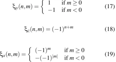
To sum up the discussion so far, by usingMaxRegain coefficients described already in Section1.2.4we al-ready have a step-wise control over the sound source spread. That can be achieved by multiplying the HOA input signal vector by a lower order set of coefficients. That in turn will a) change the relative energy ratios of channels of different order; b) zero-out higher order channel contributions. This process is visualized in Figure6.

0 1 2 3 4

Ambisonic order

0 0.2 0.4 0.6 0.8 1 1.2 1.4 1.6 1.8

Gain

MaxRe coefficients for different Ambisonic orders

order 0 order 1 order 2 order 3 order 4

Fig. 6:MaxRe gain coefficients for Ambisonic

de-coders of orders 0 to 4 (horizontal axis). Each color represents gain values (vertical axis) that each Ambisonic channel of a given order should be scaled by in order to obtain aMaxRedecoder of a given order.

However, there are two challenges with the above ap-proach. Firstly, smooth transitions between different source spreads are impossible due to Ambisonic or-ders defined as discrete values. Being able to transition smoothly between different source spreads (as opposed to keeping a constant angular spread) is critical, for ex-ample, to simulate a virtual sound source of a constant size in 3D space (for example, avolumetricsource). Secondly, the total output energy of a sound source would change when changing the spread. Recall that

MaxRecoefficients derived in Section 1.2.4ensured energy preservation when transforming between the

basicandMaxRedecoders, butnotbetween decoders of different Ambisonic orders.

To deal with the first issue, we numerically find the best polynomial approximation of eachMaxRecoefficient gain curve from figure6. This is implemented in the

set of smoothMaxRecoefficient curves is shown in Figure7.

0 0.5 1 1.5 2 2.5 3 3.5 4

Ambisonic order (fractional)

0 0.2 0.4 0.6 0.8 1 1.2 1.4 1.6 1.8

Gain

MaxRe coefficients for different Ambisonic orders

order 0 order 1 order 2 order 3 order 4

Fig. 7:MaxRe gain coefficients for fractional

Am-bisonic decoder orders ranging from 0 to 4 (hor-izontal axis). Each color represents gain values (vertical axis) that each Ambisonic channel of a given order should be scaled by in order to obtain aMaxRedecoder of a given order.

Then, we can modify the Equation24to return a frac-tional Ambisonic order which will be used by the en-coder (please note the lack of thed·eceiling operators):

n=13.15e−2.74φS ₍₂₅₎

The above formula is used in the

spread2ambiorder MATLABfunction which can be further modified if needed (for example, to allow for the relationships defined in Equations22or23).

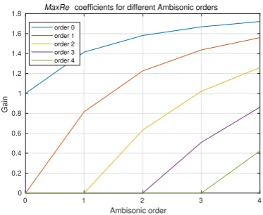
To deal with the second issue, we must ensure that when widening the sound source, we not only apply the new gain ratio to the Ambisonic channels but also the total energy of the soundfield is preserved. For example, using a maximum Ambisonic order 4 in the system, theMaxRecoefficients for Ambisonic order 4 would result in the narrowest source spread with a default amplitude. By reducing the Ambisonic order, we would make the sound source appear wider, but also quieter. To combat that, we must compensate the lower (fractional) orderMaxRecoefficients so that the sound source is equally loud, no matter how wide it is. The effect of such a compensation is illustrated in Figure8.

To compute the energy-preservingMaxRecoefficients, we first compute the energy of the soundfield at a given

0 0.5 1 1.5 2 2.5 3 3.5 4

Ambisonic order (fractional) 0

0.5 1 1.5 2 2.5 3 3.5 4 4.5 5 5.5

Gain

Energy-preserving MaxRe coefficients

order 0 order 1 order 2 order 3 order 4

Fig. 8:Energy-preservingMaxRegain coefficients for

fractional Ambisonic decoder orders ranging from 0 to 4.

Ambisonic ordern, which corresponds to the desired source spread, and compare it to the energy of the soundfield at the maximum Ambisonic orderN. The compensation gainγn,Nis a square root of this ratio:

En,N= N

∑

i=0

(2i+1)×MaxRen,N(i)2 (26)

EN,N= N

∑

i=0

(2i+1)×MaxReN,N(i)2 (27)

γn,N= s

EN,N

En,N

(28)

Finally, the energy-preserving set ofMaxRecoefficients at an arbitrary source ordernin an Ambisonic order system of orderN, is simply the raw set ofMaxRen,N

multiplied by the compensation gainγn,N.

ˆ

MaxRen,N=γn,N×MaxRen,N (29)

Of note, Resonance Audio applies the rawMaxRe cor-rection directly to the binaural decoder filters (using shelf-filters) off-line as will be explained in Section3.2. This allows for significant performance improvements at run-time. However, it means the energy-preserving

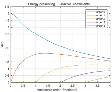
achieved by simply dividing the energy-preserving co-efficients by the coco-efficients corresponding to the max-imum Ambisonic orderN:

ˆˆ

MaxRen,N =

ˆ

MaxRen,N

MaxReN,N

(30)

The final set of coefficients is illustrated in Figure9.

0 0.5 1 1.5 2 2.5 3 3.5 4

Ambisonic order (fractional)

0 0.5 1 1.5 2 2.5 3

Gain

Energy-preserving, normalized MaxRe coefficients order 0 order 1 order 2 order 3 order 4

Fig. 9:Energy-preserving, normalizedMaxRegain

co-efficients for fractional Ambisonic decoder or-ders ranging from 0 to 4.

In Resonance Audio,maxrespread MATLAB func-tion is used to generate the energy-preserving, nor-malized MaxRe gain coefficients. The final en-coding coefficients are subsequenctly pre-computed and the LUT written into a C++-style header file using a helper MATLAB function generateco-efftable. The table is the accessed at run-time by the C++GetEncodingCoeffs method of the

AmbisonicLookupTableclass.

The drawback of the above optimization technique is that the sound source widening can result in incorrect coefficients at very low frequencies, where thebasic

decoder is in operation. To combat that, an input sound-field should be split into frequency bands at run-time and a separate set of coefficients applied to each band, which would greatly increase the CPU consumption. After informal listening tests it was decided that this inconsistency is perceptually negligible and the result of the widening process is convincing and with min-imal coloration added to the sound source. However, future work should look at evaluating these perceptual differences more formally.

2.3 Mixing in the Ambisonic domain

All sound sources within Resonance audio are mixed exclusively in the Ambisonic domain. This allows the application of all head related rotations simulta-neously and ensures that all sound sources, whether point sources encoded into soundfields, or pre-recorded soundfields, are mixed before convolution with the HRTFs. As stated, performing a fixed number of con-volutions, regardless of the number of sources, allows a large reduction in computational complexity.

To mix Ambisonic channels efficiently, Resonance Au-dio takes advantage of Single instruction multiple data (SIMD) processor instructions to add the individual samples of an Ambisonic channel to the resulting mix buffer. On Intel, the Streaming SIMD Extensions (SSE) instruction set extension; and on ARM, the NEON in-struction set, allow the execution of 128-bit inin-structions. This means that one can add four 32-bit single preci-sion floating point samples into a channel of the mix buffer simultaneously.

The related SIMD optimized code can be found in the AddPointwise function within

resonance_audio/base/simd_utils.cc.

2.4 Near-field Sound Sources

Resonance Audio also allows for simulating near-field sound sources(for example, sound sources that appear closer than the HRTF array radius which currently is 1m). Detailed description of the approximated near-field algorithm is going to be provided in a separate publication.

3

Efficient Binaural Decoding

By assuming symmetry of a human head, the complex-ity of the binaural decoding can be reduced by a factor of two compared to the approach described earlier in Section1.3.

pL=0.5 N/2

∑

i=1

[(hLi+hRi)∗(g2i−1+g2i)

+(hLi−hRi)∗(g2i−1−g2i)]

(31)

pR=0.5 N/2

∑

i=1

[(hLi+hRi)∗(g2i−1+g2i)

−(hLi−hRi)∗(g2i−1−g2i)]

(32)

From the above, we can define the convolution terms as:

c_sum,i= (hLi+hRi)∗(g2i−1+g2i) (33)

cdiff,i= (hLi−hRi)∗(g2i−1−g2i) (34)

which simplify the binaural decoding equations to:

pL=0.5 N/2

∑

i=1

(csum,i+cdiff,i) (35)

pR=0.5 N/2

∑

i=1

(csum,i−cdiff,i) (36)

Since the convolution termsc_sum,iandc_diff,iin Equa-tions35and36are identical, they are computed once. Thus, we can see that the total number of convolutions is reduced from 2Nin Equations12and13toN.

Of note, for HRIRs in the sagittal plane, we also assume left-right symmetry and hence the virtual loudspeaker contribution can be obtained by convolving the input with only one of the HRIR channels and duplicating the output to the other channel. This way, the assumption that the maximum number of convolutions equals the number of virtual loudspeakers still holds.

3.1 Symmetric HRIR convolution in the SH domain

By representing the HRIRs using SH functions and by taking advantage of the inherent symmetries and anti-symmetries of the SHs, we can further reduce the number of convolutions and make them independent of the number of HRTFs used. By doing so, we can guarantee that the maximum number of convolutions will always equal the number of SHs used in the spatial-izer. For example, for the 3rdorder Ambisonic binaural decoder using the 26-point Lebedev grid, that means reduction from 26 to 16 convolutions (∼62%).

Also, the HRTF positions in principal no longer need to conform to any symmetry. That said, the performance of the decoder is still expected to be better for regular layouts (i.e. when the loudspeaker positions are at the vertices of a platonic solid). In addition, the generation of the SH HRIRs is greatly simplified if that is the case.

In order to encode the HRIRs into SH representation, we first compute the decoding matrixDas in equation 10, where the ordering of HRTF angles follows the left-right symmetry rule: if the first HRTF is at+45◦ azimuth angle and−35.26◦elevation angle the next one should be at−45◦azimuth angle and−35.26◦, etc. The HRTFs at the sagittal plane can be added at an arbitrary order.

Next, we compose a HRIR signal matrixH, by con-catenating HRIRs in the same order that was used to compute the decoding matrixD. Following our exam-ple above, the first two columns of the matrix would be channels left and right of the HRIR corresponding to the+45◦azimuth angle and−35.26◦. The symme-try assumption means that the same HRIR is used to represent virtual loudspeakers at angles+45◦azimuth /−35.26◦elevation and−45◦azimuth /−35.26◦ ele-vation.

Finally, our SH HRIR decompositionHˆ is computed as:

ˆ

H=HDT (37)

and the binaural decoding equations for an arbitrary Ambisonic order simplify to:

pL=

∞

∑

n=0

n

∑

m=−n

pR=

∞

∑

n=0

n

∑

m=−n

bm_n ∗ˆhm

n ifm≥0

−bm_n ∗ˆhm

n ifm<0

(39)

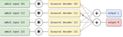
In Equation 39 the first sum over n,m corresponds to symmetric terms with respect to the forward axis, while the second sum overn,mcorresponds to anti-symmetric terms with respect to the forward axis. That is, the symmetric terms maintain their sign upon reflec-tion about the forward axis, while the anti-symmetric terms change their sign upon reflection about the for-ward axis. In practical terms, it means that the convo-lution is performed only once per Ambisonic channel, and when summing the channels to create the right ear output, channels corresponding to anti-symmetric SHs (i.e.m<0) have their phase inverted. This is illustrated in figure10for the 1st _{order Ambisonic case.}

Fig. 10:Optimized binaural decoding of Ambisonic

soundfields

3.2 Pre-filtering of SH HRIRs

The improved binaural decoding technique described above also allows for zero run-time costMaxRe sound-field optimization (see Section 1.2.4). MaxRe SH weights are typically applied using shelf-filters at the soundfield decoding stage, before the loudspeaker sig-nals are obtained. However, when using binaural decod-ing via SH HRIRs the decoddecod-ing stage is performed off-line when creating the binaural decoding filters. Hence, the shelf-filtering can also be preformed off-line once the HRIRs are represented in the SH domain. Remov-ing both decodRemov-ing matrix and shelf-filterRemov-ing from the real-time processing pipeline results in significant CPU savings and allows for efficient binaural decoding of HOA even on low-end or mobile devices.

4

Summary

This paper described the core algorithms used by the Resonance Audio’s spatializer and, at the time of writ-ing, may be used as a reference to thesource code con-tained within the Resonance Audio C++ andMATLAB

libraries. Note however, that future algorithms within the Resonance Audio might change, as new methods and DSP algorithms are constantly being developed. It is intended to record such changes as separate doc-uments referencing this paper. Also, note that not all the algorithms used by Resonance Audio have been described here, but only the ones directly pertaining to the Resonance Audio’s spatializer. For example, room effects algorithms (early reflections and late re-verberation) are mostly documented in the code itself. However, some critical parts of the late reverberation algorithm are published in [22]. Also, the near-field effect and directivity control algorithms are intended to be documented separately. Future work should fo-cus on, for example: practical ways of individualiza-tion of SH HRIRs in the Resonance Audio binaural decoder, adding efficient decoding for regular and ir-regular, physical loudspeaker setups, simulation of ad-vanced sound source radiation patterns and API meth-ods for creating volumetric sound sources, as well as further quality (for example, better modelling of spread functions at low frequencies) and efficiency improve-ments to existing algorithms.

5

Acknowledgments

The authors gratefully acknowledge Jan Skoglund, Damien Kelly, Dillon Cower, Wayne Jackson and Brian O’Toole, for their input into the project and help in preparation of this manuscript. We would also like to thank the reviewers for their insightful comments and suggestions.

References

[1] Gerzon, M. A., “Periphony: With-height sound reproduction,”Journal of the Audio Engineering Society, 21, pp. 2–10, 1973.

[2] Malham, D., “Higher order Ambisonic systems for the spatialisation of sound,” inProceedings of the International Computer Music Conference’99, Beijing, China, 1999.

[4] Nachbar, C., Zotter, F., Deleflie, E., and Son-tacchi, A., “AMBIX - A Suggested Ambisonics Format,” inProceedings of the 3rd Ambisonics Symposium, Lexington, KY, USA, 2011.

[5] Kronlachner, M.,Spatial Transformations for the Alteration of Ambisonic Recordings, Master’s the-sis, University of Music and Performing Arts, Graz, Austria, 2014.

[6] Ivanic, J. and Ruedenberg, K., “Rotation Matri-ces for Real Spherical Harmonics. Direct Deter-mination by Recursion,”The Journal of Physical Chemistry, 100(15), pp. 6342–6347, 1996, doi: 10.1021/jp953350u.

[7] Ivanic, J. and Ruedenberg, K., “Additions and Corrections: Rotation Matrices for Real Spherical Harmonics. Direct Determination by Recursion,”

The Journal of Physical Chemistry, 102(45), pp. 9099–9100, 1998, doi:10.1021/jp953350u.

[8] Green, R., “Spherical harmonic lighting: The gritty details,”Archives of the Game Developers Conference, 2003.

[9] Daniel, J., Rault, J.-B., and Polack, J.-D., “Am-bisonics Encoding of Other Audio Formats for Multiple Listening Conditions,” inProceedings of the 105th Audio Engineering Society Conven-tion, San Francisco, CA, USA, 1998.

[10] Gerzon, M. A., “General Metatheory for Auditory Localisation,” inProceedings of the 92nd Audio Engineering Society Convention, Vienna, Austria, 1992.

[11] Gerzon, M. A., “Panpot Laws for Multispeaker Stereo,” in Proceedings of the 92nd Audio En-gineering Society Convention, Vienna, Austria, 1992.

[12] Lee, R., “Shelf Filters for Ambisonic Decoders,” Technical report, http://ambisonic. info/info/ricardo/shelfs.html, 2008.

[13] Heller, A., Lee, R., and Benjamin, E., “Is My De-coder Ambisonic? (Revision 2),” inProceedings of the 125th Audio Engineering Society Conven-tion, San Francisco, CA, USA, 2008.

[14] Benjamin, E., Heller, A., and Lee, R., “Design of Ambisonic Decoders for Irregular Arrays of Loudspeakers by Non-Linear Optimization,” in

Proceedings of the 129th Audio Engineering Soci-ety Convention, San Francisco, CA, USA, 2010.

[15] McKeag, A. and McGrath, D., “Sound Field For-mat to Binaural Decoder with Head-Tracking,” in

Proceedings of the AES 6th Australian Regional Convention, Melbourne, Australia, 1996.

[16] Noisternig, M., Sontacchi, A., Musil, T., and Höldrich, R., “A 3D Ambisonic Based Binau-ral Sound Reproduction System,” inProceedings of the Audio Engineering Society 24th Interna-tional Conference on Multichannel Audio, Banff, Alberta, Canada, 2003.

[17] Dalenbäck, B. and Strömberg, M., “Real time walkthrough auralization - the first year,” Pro-ceedings of the Institute of Acoustics, 28(2), 2006.

[18] Kearney, G. and Doyle, T., “An HRTF Database for Virtual Loudspeaker Rendering,” in Proceed-ings of the 139th Audio Engineering Society Con-vention, 2015.

[19] Bertet, S., Daniel, J., Parizet, E., and Warusfel, O., “Investigation on Localisation Accuracy for First and Higher Order Ambisonics Reproduced Sound Sources,”Acta Acustica united with Acus-tica, Hirzel Verlag, 99, pp. 642–657, 2013.

[20] Epain, N., Jin, C. T., and Zotter, F., “Ambisonic Decoding With Constant Angular Spread,”Acta Acustica United with Acustica, 100, pp. 928–936, 2014.

[21] Frank, M., “Source Width of Frontal Phantom Sources: Perception, Measurement, and Model-ing,”Archives of Acoustics, 38(3), pp. 311–319, 2013.

[22] Kelly, I. J., Gorzel, M., and Güngörmüsler, A., “Efficient externalized audio reverberation with