Solving Third Order Ordinary Differential Equations Using One-Step Block Method with Four Equidistant Generalized Hybrid Points

(1)

Solving Third Order Ordinary Differential

Equations Using One-Step Block Method with

Four Equidistant Generalized Hybrid Points

Oluwaseun Adeyeye and Zurni Omar

Abstract—The application of a hybrid block method to solving third order ordinary differential equations is considered in this article. The hybrid method is developed for a set of equidistant hybrid points using a new generalized linear block method (GLBM). The equations for the GLBM takes a similar form as the conventional linear multistep method, however the form produces the needed family of schemes required to simultaneously evaluate the solution of the third order ordinary differential equations at individual grid points in a self-starting mode. The hybrid block method obtained using GLBM is investigated and the block method possesses good basic property of a numerical method which is displayed in the numerical results obtained. Furthermore, the comparison to works of the past authors shows that the new hybrid block gives impressive results in terms of error and consistency particularly for large intervals.

Index Terms—Hybrid Block Method, Generalized Linear Block Methods, Third Order, One-Step, Ordinary Differential Equations.

I. INTRODUCTION

The direct numerical approximation of general third order initial value problems (IVPs) of the form (1) below

y000=f(x, y, y0, y00), y(xn) =a, y0(xn) =b, y00(xn) =c (1) (where a, b and c are given constants) have been vastly considered in literature by several authors such as [1]–[7] amongst others. These authors focused on the direct solution of (1) due to the shortcomings of reduction to a system of three first order initial value problems which include both human and computational burden [8], [9].

Hybrid block methods are one of numerical methods adopted for directly approximating (1). It is seen to perform favourably well when numerically approximating solutions to initial value problems as it combines the advantages of block method and overcoming the zero stability barrier in linear multistep method [7].

Some authors who have presented hybrid block methods include [1], [7], [10], [11], however the generalized form for equidistant hybrid points was not attempted. In addi-tion, when considering large intervals, the numerical results obtained in comparison to the exact solution can also be improved. This informs the motivation for this article to develop a new block method with generalized equidistant

Manuscript received April 03, 2017

Corresponding Author: O. Adeyeye is a PhD candidate at Department of Mathematics, School of Quantitative Sciences, Universiti Utara Malaysia, Sintok, Kedah, Malaysia, e-mail:adeyeye oluwaseun@ahsgs.uum.edu.my

Z. Omar is a Professor of Numerical Analysis at Department of Mathe-matics, School of Quantitative Sciences, Universiti Utara Malaysia, Sintok, Kedah, Malaysia, e-mail:zurni@uum.edu.my

hybrid pointsrξ. A new linear block method is introduced in the methodology and detailed explanations on the application is discussed in the following sections.

II. DEVELOPMENT OF THEBLOCKMETHOD

Consider the generalized linear block method in the equa-tion below

yn+rξ =

2

X

i=0

(rξh)i

i! y

(i)

n +

4

X

i=0

(φξifn+ri), ξ= 1,2,3,4

(2) whose corresponding derivatives are

y(_na₊)_rξ =P3−(a+1)

i=0

(rξh)i i! y

(i+a)

n +P4_i₌₀(ωξiafn+ri); a= 1(ξ=1,2,3,4), a= 2(ξ=1,2,3,4)

(3) wherer is the distance between consecutive hybrid points, ξ represents the hybrid points which in this article is ξ = 1,2,3,4. These equations presented in equations (2) and (3) above are used to develop the hybrid block method for solving third order ordinary differential equations.

Expanding (2) and (3) yields

yn+r=yn+rhyn0 +

(rh)2 2! y

00 n

+ (φ10fn+φ11fn+r+φ12fn+2r+φ13fn+3r+φ14fn+4r) yn+2r=yn+ 2rhy0n+

(2rh)2

2! y

00 n

(3rh)2

2! y

00 n

(4rh)2

2! y

00 n

+ (φ40fn+φ41fn+r+φ42fn+2r+φ43fn+3r+φ44fn+4r) (4) y0_n₊_r=y_n0 + (rh)y_n00+ (ω101fn+ω111fn+r

+ω121fn+2r+ω131fn+3r+ω141fn+4r) y0_n₊₂_r=y_n0 + (2rh)y00_n+ (ω201fn+ω211fn+r

+ω221fn+2r+ω231fn+3r+ω241fn+4r) y0_n₊₃_r=y_n0 + (3rh)y00_n+ (ω301fn+ω311fn+r

+ω321fn+2r+ω331fn+3r+ω341fn+4r) y0n+4r=yn0 + (4rh)y00n+ (ω401fn+ω411fn+r

+ω421fn+2r+ω431fn+3r+ω441fn+4r)

y00

n+r=yn00+ (ω102fn+ω112fn+r+ω122fn+2r

+ω132fn+3r+ω142fn+4r)

y00_n₊₂_r=y_n00+ (ω202fn+ω212fn+r+ω222fn+2r

+ω232fn+3r+ω242fn+4r)

y00_n₊₃_r=y_n00+ (ω302fn+ω312fn+r+ω322fn+2r

+ω332fn+3r+ω342fn+4r)

y00_n₊₄_r=y_n00+ (ω402fn+ω412fn+r+ω422fn+2r

+ω432fn+3r+ω442fn+4r)

(5)

IAENG International Journal of Applied Mathematics, 49:2, IJAM_49_2_15

(2)

To obtain the unknown φ and ω coefficients, Taylor ex-pansion as discussed in [12] is adopted. Now, the Taylor expansion fory(_nn₊)_r=y(n)₍_xn₊_rh₎_about_xn _{is defined as}

y(n)₍_x

n+rh) =y(n)(xn) +rhy(n+1)(xn)

+(rh_2!)2y(n+2)₍_x

n) +. . .

(6)

wherey(q)(xn)₌ d q_y

dxq|x=xn, q= 1,2, . . .

Expanding each individual term in the first expression of equation (4) using equation (6) above gives

yn+ (rh)yn0 +

(rh)2

2! y

00 n+

(rh)3

3! y

000 n +

(rh)4

4! y

iv n +

(rh)5

5! y

v n

+(rh_6!)6yvi n +

(rh)7

7! y

vii

n +· · ·=yn+ (rh)yn0 +

(rh)2

2! y

00 n

+(φ10yn000+φ11(y000n + (rh)yniv+

(rh)2

2! y

v n+

(rh)3

3! y

vi n

+(rh_4!)4yvii

n +. . .) +φ12(yn000+ (2rh)yniv+

(2rh)2 2! y

v n

+(2rh_3!)3yvi n +

(2rh)4 4! y

vii

n +. . .) +φ13(yn000+ (3rh)yniv

+(3rh_2!)2yv n+

(3rh)3 3! y

vi n +

(3rh)4 4! y

vii

n +. . .) +φ14(y000n

+(4rh)yiv n +

(4rh)2 2! y

v n+

(4rh)3 3! y

vi n +

(4rh)4 4! y

vii n +. . .) which can be written in the matrix form Ax1=B1 where

A=       

1 1 1 1 1

0 (rh_1!)1 (2rh_1!)1 (3rh_1!)1 (4rh_1!)1 0 (rh_2!)2 (2rh_2!)2 (3rh_2!)2 (4rh_2!)2 0 (rh_3!)3 (2rh_3!)3 (3rh_3!)3 (4rh_3!)3 0 (rh_4!)4 (2rh_4!)4 (3rh_4!)4 (4rh_4!)4

       ,

x1=

      φ10 φ11 φ12 φ13 φ14      

, B1=

       

(rh)3

3! (rh)4

4! (rh)5

5! (rh)6

6! (rh)7

7!        

Adopting matrix inverse approach, the φ−coefficients are obtained to be

[φ10, φ11, φ12, φ13, φ14]T

=h113₁₁₂₀r3h3,107₁₀₀₈r3h3,−103r3_h3

1080 , 43r3_h3

1680 ,− 47r3_h3

10080

iT

(7) Similarly, expanding each individual term in the second expression of equation (4) using equation (6) yields

yn+ (2rh)y0_n+(2rh_2!)2y00_n+(2rh_3!)3y_n000+(2rh_4!)4yiv n +

(2rh)5 5! y

v n

+(2rh_6!)6yvi n +

(2rh)7 7! y

vii

n +· · ·=yn+ (2rh)y0n+

(2rh)2 2! y

00 n

+(φ20yn000+φ21(y000n + (rh)y iv n +

(rh)2 2! y

v n+

(rh)3 3! y

vi n

+(rh_4!)4y_nvii+. . .) +φ22(yn000+ (2rh)y iv n +

(2rh)2 2! y

v n

+(2rh_3!)3ynvi+

(2rh)4 4! y

vii

n +. . .) +φ23(yn000+ (3rh)yniv

+(3rh_2!)2ynv+

(3rh)3

3! y

vi n +

(3rh)4

4! y

vii

n +. . .) +φ24(y000n

+(4rh)yniv+

(4rh)2

2! y

v n+

(4rh)3

3! y

vi n +

(4rh)4

4! y

vii n +. . .) with corresponding matrix formAx2=B2 where

x2=

      φ20 φ21 φ22 φ23 φ24      

, B2=

       

(2rh)3

3! (2rh)4

4! (2rh)5

5! (2rh)6

6! (2rh)7

7!        

The resulting φ−coefficients from matrix inverse approach are

[φ20, φ21, φ22, φ23, φ24]

T

=h331₆₃₀r3h3,332₃₁₅r3h3,−8r3h3

21 , 52r3h3

315 ,− 19r3h3

630

iT (8)

Considering the third expression of equation (4), individual terms are expanded using equation (6) to obtain

yn+ (3rh)yn0 +

(3rh)2

2! y

00 n+

(3rh)3

3! y

000 n +

(3rh)4

4! y

iv n

+(3rh_5!)5yv n+

(3rh)6

6! y

vi n +

(3rh)7

7! y

vii

n +· · ·=yn+ (3rh)y0n

+(3rh_2!)2y00_n+ (φ30yn000+φ31(yn000+ (rh)yniv+

(rh)2

2! y

v n

+(rh_3!)3yvi n +

(rh)4 4! y

vii

n +. . .) +φ32(y000n + (2rh)yniv

+(2rh_2!)2yv n+

(2rh)3 3! y

vi n +

(2rh)4 4! y

vii

n +. . .) +φ33(yn000

+(3rh)yiv n +

(3rh)2 2! y

v n+

(3rh)3 3! y

vi n +

(3rh)4 4! y

vii n +. . .)

+φ34(y000n + (4rh)yivn +

(4rh)2 2! y

v n+

(4rh)3 3! y

vi n

+(4rh_4!)4yvii n +. . .)

having matrix formAx3=B3 with

x3=

      φ30 φ31 φ32 φ33 φ34      

, B3=

       

(3rh)3

3! (3rh)4

4! (3rh)5

5! (3rh)6

6! (3rh)7

7!         and

[φ30, φ31, φ32, φ33, φ34]

T

=h1431₁₁₂₀r3h3,1863₅₆₀r3h3,−243r3h3

560 , 45r3h3

112 ,− 81r3h3

1120

iT

(9) Likewise, considering the fourth and last expression of equation (4), individual terms are expanded using equation (6) to obtain

yn+ (4rh)y_n0 +(4rh_2!)2y00_n+(4rh_3!)3y_n000+(4rh_4!)4yiv n

+(4rh_5!)5yv n+

(4rh)6 6! y

vi n +

(4rh)7 7! y

vii

n +· · ·=yn

+(4rh)y_n0 +(4rh_2!)2y00_n+ (φ40y000n +φ41(yn000+ (rh)yivn

+(rh_2!)2yv n+

(rh)3 3! y

vi n +

(rh)4 4! y

vii

n +. . .) +φ42(y000n

+(2rh)y_niv+(2rh_2!)2y_nv+(2rh_3!)3yvi_n +(2rh_4!)4yvii_n +. . .) +φ43(y000n + (3rh)y

iv n +

(3rh)2 2! y

v n+

(3rh)3 3! y

vi n

+(3rh_4!)4ynvii+. . .) +φ44(yn000+ (4rh)yniv+

(4rh)2 2! y

v n

+(4rh_3!)3ynvi+

(4rh)4

4! y

vii n +. . .) written in the matrix formAx4=B4,

x4=

      φ40 φ41 φ42 φ43 φ44      

, B4=

       

(4rh)3 3! (4rh)4

4! (4rh)5

5! (4rh)6

6! (4rh)7

7!        

and Theφ−coefficients are obtained as

[φ40, φ41, φ42, φ43, φ44]

T

=h248₁₀₅r3h3,2176₃₁₅r3h3,32₁₀₅r3h3,128₁₀₅r3h3,−8r3_h3

63

iT (10)

Moving on to obtaining theω−coefficients in equation (5). Expanding each individual term in the first expression of

IAENG International Journal of Applied Mathematics, 49:2, IJAM_49_2_15

(3)

equation (5) using equation (6) above gives

y_n0 + (rh)y_n00+(rh_2!)2y000_n +(rh_3!)3yiv n +

(rh)4

4! y

v n+

(rh)5

5! y

vi n

+(rh_6!)6yvii

n +· · ·=yn0 + (rh)yn00+ (ω101y000n +ω111(y000n

+(rh)yiv n +

(rh)2

2! y

v n+

(rh)3

3! y

vi n +

(rh)4

4! y

vii n +. . .)

+ω121(yn000+ (2rh)yniv+

(2rh)2 2! y

v n+

(2rh)3 3! y

vi n +

(2rh)4 4! y

vii n

+. . .) +ω131(y000n + (3rh)yivn +

(3rh)2 2! y

v n+

(3rh)3 3! y

vi n

+(3rh_4!)4yvii

n +. . .) +ω141(y000n + (4rh)yivn +

(4rh)2 2! y

v n

+(4rh_3!)3yvi n +

(4rh)4 4! y

vii n +. . .)

which can be written in the matrix form Ax5=B5 where

x5=

      ω101 ω111 ω121 ω131 ω141      

, B5=

       

(rh)2

2! (rh)3

3! (rh)4

4! (rh)5

5! (rh)6

6!        

and The matrix inverse approach is also adopted to obtain the ω−coefficients as

[ω101, ω111, ω121, ω131, ω141]T

=h367₁₄₄₀r2h2,3r₈2h2,−47r2_h2

240 , 29r2_h2

360 ,− 7r2_h2

480

iT (11)

For the second expression in equation (5), each individual term are likewise expanded using equation (6) to obtain

y_n0 + (2rh)y00_n+(2rh_2!)2y000_n +(2rh_3!)3yiv n +

(2rh)4 4! y

v n

+(2rh_5!)5y_nvi+(2rh_6!)6y_nvii+· · ·=y_n0 + (2rh)y00_n+ (ω201yn000

+ω211(yn000+ (rh)y iv n +

(rh)2 2! y

v n+

(rh)3 3! y

vi n +

(rh)4 4! y

vii n

+. . .) +ω221(y000n + (2rh)y iv n +

(2rh)2 2! y

v n+

(2rh)3 3! y

vi n

+(2rh_4!)4ynvii+. . .) +ω231(y000n + (3rh)yivn +

(3rh)2 2! y

v n

+(3rh_3!)3ynvi+

(3rh)4

4! y

vii

n +. . .) +ω241(y000n + (4rh)yivn

+(4rh_2!)2ynv+

(4rh)3

3! y

vi n +

(4rh)4

4! y

vii n +. . .)

which can be written in the matrix form Ax6=B6 where

x6=

      ω201 ω211 ω221 ω231 ω241      

, B6=

       

(2rh)2

2! (2rh)3

3! (2rh)4

4! (2rh)5

5! (2rh)6

6!         and

[ω201, ω211, ω221, ω231, ω241]

T

=h53r₉₀2h2,8r2₅h2,−r2h2

3 , 8r2h2

45 ,−

r2h2

30

iT (12)

Moving to the third expression in equation (5). In same manner, equation (6) and (7) are adopted to expand its individual terms to obtain

y0

n+ (3rh)y00n+

(3rh)2

2! y

000 n +

(3rh)3

3! y

iv n +

(3rh)4

4! y

v n

+(3rh_5!)5yvi n +

(3rh)6

6! y

vii

n +· · ·=y0n+ (3rh)yn00

+(ω301y000n +ω311(y000n + (rh)yniv+

(rh)2

2! y

v n+

(rh)3

3! y

vi n

+(rh_4!)4yvii

n +. . .) +ω321(y000n + (2rh)yivn +

(2rh)2

2! y

v n

+(2rh_3!)3yvi n +

(2rh)4

4! y

vii

n +. . .) +ω331(y000n + (3rh)yivn

+(3rh_2!)2yv n+

(3rh)3

3! y

vi n +

(3rh)4

4! y

vii

n +. . .) +ω341(yn000

+(4rh)yiv n +

(4rh)2

2! y

v n+

(4rh)3

3! y

vi n +

(4rh)4

4! y

vii n +. . .)

in the matrix formAx7=B7 where

x7=

      ω301 ω311 ω321 ω331 ω341      

, B7=

       

(3rh)2

2! (3rh)3

3! (3rh)4

4! (3rh)5

5! (3rh)6

6!         and

[ω301, ω311, ω321, ω331, ω341]

T

=h147r2h2

160 , 117r2h2

40 , 27r2h2

80 , 3r2h2

8 ,− 9r2h2

160

iT (13)

Now consider the fourth expression in equation (5), which is the last expression for the first derivative schemes. Individual terms are also expanded using equation (6) to obtain

y0n+ (4rh)yn00+

(4rh)2

2! y

000 n +

(4rh)3

3! y

iv n +

(4rh)4

4! y

v n

+(4rh_5!)5yvi n +

(4rh)6

6! y

vii

n +· · ·=yn0 + (4rh)y00n

+(ω401yn000+ω411(yn000+ (rh)yivn +

(rh)2

2! y

v n+

(rh)3

3! y

vi n

+(rh_4!)4yvii

n +. . .) +ω421(yn000+ (2rh)yivn +

(2rh)2

2! y

v n

+(2rh_3!)3yvi n +

(2rh)4

4! y

vii

n +. . .) +ω431(yn000+ (3rh)yivn

+(3rh_2!)2yv n+

(3rh)3

3! y

vi n +

(3rh)4

4! y

vii

n +. . .) +ω441(y000n

+(4rh)yiv n +

(4rh)2

2! y

v n+

(4rh)3

3! y

vi n +

(4rh)4

4! y

vii n +. . .) which can be written in the matrix formAx8=B8 where

x8=

      ω401 ω411 ω421 ω431 ω441      

, B8=

       

(4rh)2

2! (4rh)3

3! (4rh)4

4! (4rh)5

5! (4rh)6

6!        

with resultingω−coefficients obtained to be

[ω401, ω411, ω421, ω431, ω441]

T

=h56r₄₅2h2,64r₁₅2h2,16r₁₅2h2,64r₄₅2h2,0i

T ₍₁₄₎

The fifth expression in equation (5) is the first expression for the second derivative schemes. Expanding each individual term in this fifth expression of equation (5) using equation (6) above gives

y00

n+ (rh)y000n +

(rh)2

2! y

iv n +

(rh)3

3! y

v n+

(rh)4

4! y

vi n +

(rh)5

5! y

vii n

+· · ·=y_n00+ (ω102y000n +ω112(yn000+ (rh)yniv+

(rh)2

2! y

v n

+(rh_3!)3yvi n +

(rh)4

4! y

vii

n +. . .) +ω122(yn000+ (2rh)yniv

+(2rh_2!)2yv n+

(2rh)3

3! y

vi n +

(2rh)4

4! y

vii

n +. . .) +ω132(y000n

+(3rh)yiv n +

(3rh)2

2! y

v n+

(3rh)3

3! y

vi n +

(3rh)4

4! y

vii n +. . .)

+ω142(y000n + (4rh)yniv+

(4rh)2

2! y

v n+

(4rh)3

3! y

vi n

+(4rh_4!)4yvii n +. . .)

implying the matrix formAx9=B9 with

x9=

      ω102 ω112 ω122 ω132 ω142      

, B9=

       

(rh)1

1! (rh)2

2! (rh)3

3! (rh)4

4! (rh)5

5!        

Theω−coefficients are obtained to be

[ω102, ω112, ω122, ω132, ω142]

T

=251rh

720 , 323rh

320 ,− 11rh

30 , 53rh

360,− 19rh

720

T (15)

IAENG International Journal of Applied Mathematics, 49:2, IJAM_49_2_15

(4)

Similarly, expanding each individual term in the sixth ex-pression in equation (5) using equation (6) yields

y_n00+ (2rh)y000_n +(2rh_2!)2y_niv+(2rh_3!)3y_nv+(2rh_4!)4yvi_n

+(2rh_5!)5ynvii+· · ·=yn00+ (ω202y000n +ω212(y000n + (rh)yniv

+(rh_2!)2ynv+

(rh)3 3! y

vi n +

(rh)4 4! y

vii

n +. . .) +ω222(yn000

+(2rh)yniv+

(2rh)2

2! y

v n+

(2rh)3

3! y

vi n +

(2rh)4

4! y

vii n +. . .)

+ω232(yn000+ (3rh)yniv+

(3rh)2

2! y

v n+

(3rh)3

3! y

vi n

+(3rh_4!)4yvii

n +. . .) +ω242(y000n + (4rh)yivn +

(4rh)2

2! y

v n

+(4rh_3!)3yvi n +

(4rh)4

4! y

vii n +. . .)

with corresponding matrix formAx10=B10 where

x10=

      ω202 ω212 ω222 ω232 ω242      

, B10=

       

(2rh)1

1! (2rh)2

2! (2rh)3

3! (2rh)4

4! (2rh)5

5!         and

[ω202, ω212, ω222, ω232, ω242]

T

=29rh

90 , 62rh 45 , 4rh 15, 2rh

360,−

rh

90

T (16)

For the seventh expression in equation (5), individual terms are expanded using equation (6) to obtain

yn00+ (3rh)y000n +

(3rh)2

2! y

iv n +

(3rh)3

3! y

v n+

(3rh)4

4! y

vi n

+(3rh_5!)5ynvii+· · ·=yn00+ (ω302y000n +ω312(y000n + (rh)yniv

+(rh_2!)2ynv+

(rh)3

3! y

vi n +

(rh)4

4! y

vii

n +. . .) +ω322(yn000

+(2rh)yiv n +

(2rh)2

2! y

v n+

(2rh)3

3! y

vi n +

(2rh)4

4! y

vii n +. . .)

+ω332(yn000+ (3rh)yniv+

(3rh)2

2! y

v n+

(3rh)3

3! y

vi n +

(3rh)4

4! y

vii n

+. . .) +ω342(y000n + (4rh)yivn +

(4rh)2

2! y

v n+

(4rh)3

3! y

vi n

+(4rh_4!)4yvii n +. . .)

written in the matrix form Ax11=B11 where

x11=

      ω302 ω312 ω322 ω332 ω342      

, B11=

       

(3rh)1

1! (3rh)2

2! (3rh)3

3! (3rh)4

4! (3rh)5

5!         and

[ω302, ω312, ω322, ω332, ω342]

T

=27₈₀rh,51₄₀rh,9₁₀rh,21₄₀rh,−3rh

80

T (17)

Finally, for the eighth expression in equation (5) which is the last expression for the derivative schemes, individual terms are also expanded using equation (6) as given

y00

n+ (4rh)y000n +

(4rh)2

2! y

iv n +

(4rh)3

3! y

v n+

(4rh)4

4! y

vi n

+(4rh_5!)5yvii

n +· · ·=yn00+ (ω402y000n +ω412(y000n + (rh)yniv

+(rh_2!)2yv n+

(rh)3

3! y

vi n +

(rh)4

4! y

vii

n +. . .) +ω422(yn000

+(2rh)yiv n +

(2rh)2

2! y

v n+

(2rh)3

3! y

vi n +

(2rh)4

4! y

vii n +. . .)

+ω432(yn000+ (3rh)yniv+

(3rh)2

2! y

v n+

(3rh)3

3! y

vi n

+(3rh_4!)4yvii

n +. . .) +ω442(y000n + (4rh)yivn +

(4rh)2

2! y

v n

+(4rh_3!)3yvi n +

(4rh)4

4! y

vii n +. . .)

with corresponding matrix formAx12=B12 where

x12=

      ω402 ω412 ω422 ω432 ω442      

, B12=

       

(4rh)1

1! (4rh)2

2! (4rh)3

3! (4rh)4

4! (4rh)5

5!         and

[ω402, ω412, ω422, ω432, ω442]T

=14rh

45 , 64rh 45 , 8rh 15, 64rh 45 , 14rh 45 T (18)

Substituting the values obtained for the unknown coefficients in equations (7), (8), (9) and (10), into equation (4) gives the block form

I4Ynr=A1Zn+A2Zn1+A3Zn2+B1Fn+B2Fnr (19)

where

I4=



  

1 0 0 0

0 1 0 0

0 0 1 0

0 0 0 1



  

, Ynr = 

  

yn+r yn+2r yn+3r yn+4r



  

,

A1=



  

0 0 0 1



  

, Zn=



  

yn−3r yn−2r yn−r

yn



  

A2=



  

0 0 0 rh

0 0 0 2rh

0 0 0 3rh

0 0 0 4rh



  

, Zn1=



  

y_n0₋₃_r y_n0₋₂_r y_n0₋_r

y0_n



  

,

A3=



   

0 0 0 (rh_2!)2 0 0 0 (2rh_2!)2 0 0 0 (3rh_2!)2 0 0 0 (4rh_2!)2



   

, Zn2=



  

y00n−3r y00

n−2r y00

n−r y_n00



  

B1=



   

0 0 0 113r3h3

1120

0 0 0 331₆₃₀r3h3 0 0 0 1431₁₁₂₀r3h3 0 0 0 248₁₀₅r3h3



   

, Fn = 

  

fn−3r fn−2r fn−r

fn     ,

B2=



   

107r3_h3

1008 −

103r3_h3

1680

43r3_h3

1680 −

47r3_h3

10080 332r3_h3

315 −

8r3_h3

21

52r3_h3

315 −

19r3_h3

630 1863r3h3

560 −

243r3h3

560

45r3h3

112 −

81r3h3

1120 2176r3_h3

315

32r3_h3

105

128r3_h3

105 −

8r3_h3

63      ,

and Fnr=



  

fn+r fn+2r fn+3r fn+4r



  

.

Substituting the values obtained for the unknown coefficients in equations (10)-(18), into equation (5) gives the block form

I4Y (1)

nr =A1Zn1+A2Zn2+B (1) 1 Fn+B

(1) 2 Fnr

I4Y (2)

nr =A1Zn2+B (2) 1 Fn+B

(2)

2 Fnr

(20)

IAENG International Journal of Applied Mathematics, 49:2, IJAM_49_2_15

(5)

where

I4=



  

1 0 0 0

0 1 0 0

0 0 1 0

0 0 0 1



  

, Ynr(1)=



  

yn0+r yn0+2r yn0+3r y0

n+4r



  

,

A1=



  

0 0 0 1



  

, Zn1=



  

yn0−3r yn0−2r

y0 n−r y0_n



  

A2=



  

0 0 0 rh

0 0 0 2rh

0 0 0 3rh

0 0 0 4rh



  

, Zn2=



  

y00 n−3r y00

n−2r y00_n₋_r

y_n00



  

,

B₁(1)= 

   

0 0 0 367₁₄₄₀r2h2 0 0 0 53r₉₀2h2 0 0 0 147₁₆₀r2h2 0 0 0 56r₄₅2h2



   

, Fn= 

  

fn−3r fn−2r fn−r

fn



  

,

B₂(1)= 

   

3r2h2

8 −

47r2h2

240

29r2h2

360 −

7r2h2

480 8r2_h2

5 −

r2_h2

3

8r2_h2

45 −

r2_h2

30 117r2_h2

40

27r2_h2

80

3r2_h2

8 −

9r2_h2

160 64r2h2

15

16r2h2

15

64r2h2

45 0



   

,

Fnr= 

  

fn+r fn+2r fn+3r fn+4r



  

, Ynr(2)=



  

y00 n+r y00

n+2r y_n00₊₃_r y_n00₊₄_r



  

,

B₁(2)= 

  

0 0 0 251₇₂₀rh 0 0 0 29₉₀rh 0 0 0 27₈₀rh 0 0 0 14₄₅rh



  

, and

B(2)₂ = 

  

323rh

360 −

11rh

30 53rh

360 −

19rh

720 62rh

45

4rh

15

2rh

45 −

rh

90 51rh

40

9rh

10

21rh

40 −

3rh

80 64rh

45

8rh

15

64rh

45

14rh

45



  

.

III. ANALYSIS OF THEBLOCKMETHOD

In this section, the properties investigated for the block method will be limited to the properties needed to ensure the block method is convergent. As conventionally known, a linear multistep method is convergent iff it is consistent and zero-stable [13]

Definition 3.1: A linear multistep method isconsistent if it has order p≥1.

A. Order of the Block Method

To obtain the order of the block method, the y and f−

values in equation (19) are expanded to obtain

P7

i=0 (rξh)i

i! y (i)

n −P2_i₌₀(rξh) i i! y

(i)

n

−P4

j=0φξj

P7

i=3 (rξh)i

i! y (i)

n

;ξ= 1,2,3,4 = [0,0,0,0]

(21)

This gives the order of the block method to be of order

[5,5,5,5]T with error constants[139₄₀₃₂₀r8,r₄₅8,243₄₄₈₀r8,32₃₁₅r8]

B. Zero-Stability of the Block Method

To analyze the block method (19) for zero stability, the roots of the first characteristic polynomialρ(r) =|rI4−A1|

must be simple or less than one. This implies that

ρ(r) =|rI4−A1|

=

r



  

1 0 0 0

0 1 0 0

0 0 1 0

0 0 0 1



  

−



  

0 0 0 1



  

=r3(r−1)

which has rootsr= 0,0,0,1and this implies that the block method is zero-stable.

C. Convergence of the Block Method

The block method is consistent and zero-stable, hence the block method is convergent.

IV. NUMERICALEXAMPLES

Problem 1: y000 + ex = 0, y(0) = 1, y0(0) =

−1, y00(0) = 3.

Exact solution:y(x) = 2x2−ex+ 2 withh= 0.1.

This third order initial value problem was solved by [7] using an hybrid block method of order 5.

Problem 2: y000 + 4y0 = x, y(0) = y0(0) = 0, y00(0) = 1.

Exact solution:y(x) =₁₆3(1−cos 2x) +1₈x2

This third order initial value problem was solved by [11] using a combination of predictor of order 6 and the corrector of order 7 and also [2].

Problem 3: y000 + y = 0, y(0) = 1, y0(0) =

−1, y00(0) = 1,[0,1].

Exact solution:y(x) =e−x+ 2withh= 0.1.

This third order initial value problem was solved by [5] and [7] using block methods of order 8 and 5 respectively. The maximum error at the end of the interval is considered

Problem 4: y000 − xy00 + x2_y2 ₌ _xsinx ₋ _cosx ₊

x2_sin2_x, _y_{(0) = 0}_, _y0_{(0) = 1}_, _y00_{(0) = 0}_,_[0_,_1]_. Exact solution:y(x) =sinxwithh= 0.1.

This nonlinear initial value problem in third order ordinary differential equation was sourced from [14].

Problem 5: y000 = ₈3_y5, y(x0) = 0, y0(x0) = 1

2, y

00₍_x

0) =−1₄ where0≤x≤2.

Exact solution:y(x) =√1 +xwithh= 0.1.

This special nonlinear initial value problem in third order ordinary differential equation was sourced from [15]. The authors did not provide a numerical approximation of this problem, thus Table 5 displays only the numerical solution using the hybrid block method in comparison to the exact solution.

IAENG International Journal of Applied Mathematics, 49:2, IJAM_49_2_15

(6)

[image:6.595.48.351.71.195.2]

Table 1: Comparison of results with [7] for solving Problem 1

x Exact Solution Computed Solution withr=1₄

Error [7] Error (Hybrid Block Method) 0.1 0.91482908192435231 0.91482908192436851 1.110223E-14 1.620926E-14 0.2 0.85859724183983022 0.85859724183989627 1.607603E-13 6.605827E-14 0.3 0.83014119242399698 0.83014119242414974 6.310508E-13 1.527667E-13 0.4 0.82817530235872971 0.82817530235900927 1.623146E-12 2.795542E-13 0.5 0.85127872929987181 0.85127872930032200 3.359091E-12 4.501954E-13 0.6 0.89788119960949109 0.89788119961015944 6.084133E-12 6.683543E-13 0.7 0.96624729252952335 0.96624729253046260 1.006994E-11 9.392487E-13 0.8 1.05445907150753240 1.05445907150879940 1.561595E-11 1.266987E-12 0.9 1.16039688884305030 1.16039688884470800 2.305356E-11 1.657785E-12 1.0 1.28171817154095450 1.28171817154307190 3.274958E-11 2.117417E-12

Table 2: Comparison of results for solving Problem 2

Awoyemi (2003) Zanariah et al (2012) Hybrid Block Method with

r=1 4

Step-size

b TS Maximum Error

[image:6.595.303.549.411.622.2]

0.025 5.0 200 3.94E-6 5.0 46 4.66E-7 5.0 46 1.20E-10 56 9.14E-8 56 3.69E-11 88 1.53E-10 88 2.44E-12 0.025 10.0 400 3.80E-6 10.0 61 4.66E-7 10.0 61 5.54E-09 91 2.43E-8 91 5.04E-10 136 1.53E-10 136 4.53E-11 0.025 15.0 600 2.29E-6 15.0 76 4.66E-7 15.0 76 2.67E-08 110 2.63E-8 110 2.91E-09 180 1.54E-10 180 1.52E-10 0.025 20.0 800 1.30E-6 20.0 91 4.66E-7 20.0 91 5.29E-08 129 2.63E-8 129 6.54E-09 204 1.28E-9 204 4.19E-10

Table 3: Comparison of results with [5] and [7] for solving Problem 3

Maximum Error [5] 8.200535E-11

Maximum Error [7] 3.443523E-12

Maximum Error (Hybrid Block Method with r= 1₄)

1.184275E-12

x Exact Solution Computed Solution withr=1

4

Error (Hybrid Block Method) 0.1 0.099833416646828155 0.099833416646827489 6.661338E-16 0.2 0.198669330795061220 0.198669330795057300 3.913536E-15 0.3 0.295520206661339600 0.295520206661327170 1.243450E-14 0.4 0.389418342308650520 0.389418342308621660 2.886580E-14 0.5 0.479425538604203010 0.479425538604146990 5.601075E-14 0.6 0.564642473395035370 0.564642473394938450 9.692247E-14 0.7 0.644217687237691020 0.644217687237536360 1.546541E-13 0.8 0.717356090899522680 0.717356090899290090 2.325917E-13 0.9 0.783326909627483300 0.783326909627148680 3.346212E-13 1.0 0.841470984807896390 0.841470984807431990 4.644063E-13

Problems 1 to 5 have considered sample third order ODEs ranging from linear to nonlinear problems. The results displayed of each Problem are displayed in Tables 1 to 5 respectively and the hybrid block methods shows impressive accuracy when compares to other authors. For Problem 5, [15] displayed the maximum error for solving Problem 5 using a five-step explicit method as

1.02939×10−7 over the defined interval.

x Exact Solution Computed Solution withr=1₄

Error (Hybrid Block Method) 0.1 1.048808848170151600 1.048808848176159900 6.008305E-12 0.2 1.095445115010332100 1.095445115032145100 2.181300E-11 0.3 1.140175425099138100 1.140175425143080500 4.394241E-11 0.4 1.183215956619923200 1.183215956690615500 7.069234E-11 0.5 1.224744871391588900 1.224744871492748900 1.011600E-10 0.6 1.264911064067351800 1.264911064202180800 1.348290E-10 0.7 1.303840481040529700 1.303840481211909800 1.713800E-10 0.8 1.341640786499873800 1.341640786710470700 2.105969E-10 0.9 1.378404875209022100 1.378404875461343400 2.523213E-10 1.0 1.414213562373095100 1.414213562669522500 2.964273E-10 1.1 1.449137674618943700 1.449137674961753900 3.428102E-10 1.2 1.483239697419132600 1.483239697810508700 3.913760E-10 1.3 1.516575088810310000 1.516575089252350800 4.420408E-10 1.4 1.549193338482966800 1.549193338977691300 4.947245E-10 1.5 1.581138830084189800 1.581138830633542500 5.493528E-10 1.6 1.612451549659710000 1.612451550265563600 6.058536E-10 1.7 1.643167672515498400 1.643167673179656700 6.641583E-10 1.8 1.673320053068151300 1.673320053792351400 7.242000E-10 1.9 1.702938636592640200 1.702938637378554900 7.859147E-10 2.0 1.732050807568877400 1.732050808418116800 8.492393E-10

Therefore, the new hybrid block method has better accuracy with its maximum error of8.492393×10−10_.

To further show the usability of the hybrid block method, certain benchmark models of third order ODEs are considered as discussed in the following sections.

IAENG International Journal of Applied Mathematics, 49:2, IJAM_49_2_15

(7)

V. APPLICATION TOSOLVENONLINEARGENESIO

EQUATION

The section considers the non-linear chaotic system from [16]

x000+Ax00+Bx0−f(x(t)) = 0 (22)

with

f(x(t)) =−Cx(t) +x2(t) (23)

subject to the following conditions:

x(0) = 0.2, x0(0) =−0.3, x00(0) = 0.1, t∈[0, b]

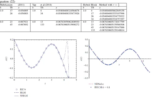
[image:7.595.314.538.111.270.2]

where A = 1.2, B = 2.92 and C = 6 are positive constants satisfying AB < C to guarantee the existence of the solution of (22). The new hybrid block method is adopted to solve (22) in self-starting mode where the block method simultaneously integrates (22) at all grid points. The numerical results obtained from the new hybrid block method are compared with the solutions obtained in [17]–[19]. Table 6 shows the comparison in the numerical approximation of x at the end points b = 1 and b = 4. It is the observed that the new hybrid block method obtains convergent results as [17] variable step three-point block multistep method and [19] block hybrid collocation method. Figure 2 displays the numerical solutions for the nonlinear Genesio equation (22) in the interval [0, 4.5] as depicted in the separate works of [18] and [19]. The numerical approximations obtained by the new hybrid block method is further seen to be in agreement with the authors.

Table 6:Comparison of results for the nonlinear Genesio equation (22)

Mehrkanoon (2011) Yap et al (2014) Hybrid Block Method withr=1₄

b TS x b TS x b TS x

1.0 17 -0.054005 1.0 4 -0.05400408324564678 1.0 4 -0.054004085662849158 26 -0.054003 34 -0.05400408355473926 17 -0.054004083555107996 26 -0.054004083554779522 34 -0.054004083554757297 4.0 23 -0.067921 4.0 13 -0.06763059062408930 4.0 13 -0.067630605172017799 45 -0.067692 133 -0.06763060515900272 23 -0.067630605159560306 45 -0.067630605159147886 133 -0.067630605159140614

Fig. 1. Solutions obtained for (22) using seven- and eight-order Runge Kutta method (RK78), homotopy analysis method (HAM), new variant of HAM (NHAM) [18] and block hybrid collocation method [19]

-0.25 -0.2 -0.15 -0.1 -0.05 0 0.05 0.1 0.15 0.2 0.25

0 0.5 1 1.5 2 2.5 3 3.5 4 4.5 5

x(

t)

t

Hybrid Block Method

Fig. 2. Solutions obtained for (22) using Hybrid Block Method

IAENG International Journal of Applied Mathematics, 49:2, IJAM_49_2_15

[image:7.595.53.542.419.736.2]

(8)

VI. APPLICATION TOSOLVEPROBLEM INTHINFILM

FLOW

Consider the problem concerned with the flow of thin films of viscous fluid with a free surface in which surface tension effects play a role typically leading to third-order ordinary differential equations governing the shape of the free surface of the fluid, y = y(x). One of such equation is the fluid dynamics problem formulated as an autonomous third order ODE

y000=f(y) (24)

where

f(y) =−1 +y−2_,

f(y) =−1 + (1 +δ+δ2₎_y−2₋₍_δ₊_δ2₎_y−3_,

f(y) =y−2₋_y−3_,

f(y) =y−2_.

(25)

Numerical methods for solving third order ODEs have been extended to solve these resultant third order ODE problem in thin film flow [20] of the form

y000=y−k (26)

with initial conditions y(0) = y0(0) = y00(0) = 1 for the casesk= 2 andk= 3.

[20] applied the three-stage fifth order Runge Kutta method to solve the third order physical problem (27) directly while [21] adopted the seven-stage fifth-order Runge-Kutta. The new hybrid block method is also applied to solve (27) directly. The results are presented in the following tables in comparison to [21] and [20].

Table 7:Numerical results for problem in Thin Film Flow (27) withh= 0.01,k= 2

x Exact Solu-tion

Error [21] Error [20] Error (Hybrid Block Method) 0.0 1.000000000 1.0000000000 1.0000000000 1.0000000000 0.2 1.221211030 1.2212100045 1.2212100045 1.2212100045 0.4 1.488834893 1.4888347799 1.4888347799 1.4888347799 0.6 1.807361404 1.8073613977 1.8073613977 1.8073613977 0.8 2.179819234 2.1798192339 2.1798192339 2.1798192339 1.0 2.608275822 2.6082748676 2.6082748676 2.6082748676

Table 7 demonstrates that the new hybrid block method is suitable to solve the thin film flow model withh= 0.01and k = 2. This is observed in the convergent results between the [21], [20] and the new hybrid block method.

The next case considered if for k= 3 withh= 0.01. This case actual has no analytic solution. Table 8 shows the numerical results.

Table 8:Numerical results for problem in Thin Film Flow (27) withh= 0.01,k= 3

x Error [21] Error [20] Error (Hybrid Block Method) 0.0 1.0000000000 1.0000000000 1.0000000000 0.2 1.2211551424 1.2211551423 1.2211551424 0.4 1.4881052842 1.4881052838 1.4881052842 0.6 1.8042625481 1.8042625471 1.8042625481 0.8 2.1715227981 2.1715227960 2.1715227981 1.0 2.5909582591 2.5909582556 2.5909582591

As a result of the inability to obtain the exact solution to (27) for k = 3, comparison is made between the adopted approaches. Further convergence is also displayed by the

new hybrid block method in Table 8. The results obtained by the hybrid block method are exactly same to [21] although the three-stage fifth order Runge Kutta method by [20] also gave close results.

VII. CONCLUSION

From the tables above, the hybrid block method has shown better accuracy with less and equal number of steps in comparison to [2] and [11] respectively. Also, in comparison to previous existing methods having equal and higher order [5], [7], [15], the hybrid block method has also competed favourably. The properties of convergence and consistency can also been seen from the numerical results. In addition, the suitability of the hybrid block method in application to the nonlinear Genesio equation and the physical problem modelling thin film flow was also investigated. Convergence in solution and improved accuracy were properties displayed by the hybrid block method when solving these additional models. Thus, this new generalized hybrid block method suitable for numerical approximation of third order initial value problems.

ACKNOWLEDGMENT

This work was supported by Universiti Utara Malaysia.

REFERENCES

[1] D. O. Awoyemi and O. M.Idowu, “A class of hybrid collocation methods for third-order ordinary differential equations,” Journal of Computer

Mathematics, vol. 82, no. 1, pp. 1287-1293, 2005.

[2] D. O. Awoyemi, “A P-stable linear multistep method for solving general third order ordinary differential equations,” International Journal of

Computer Mathematics, vol. 80, no. 8, pp. 985-991, 2003.

[3] A. O. Adesanya and B. Abdulqadri and Y. S. Ibrahim, “Hybrid one step block method for the solution of third order initial value problems of ordinary differential equations,” International Journal of Applied

Mathematics and Computation, vol. 6, no. 1, pp. 10-16, 2005.

[4] M. O. Udoh and D. O. Awoyemi, “An algorithm for solving initial value problems of third order ordinary differential equations,”Global Journal

of Mathematical Sciences, vol. 8, no. 2, pp. 123-130, 2009.

[5] Z. Omar and J. O. Kuboye, “Developing block method of order seven for solving third order ordinary differential equations directly using multistep collocation approach,”International Journal of Applied

Mathematics and Statistics, vol. 53, no. 3, pp. 165-173, 2015.

[6] U. Mohammed and R. B. Adeniyi, “A three step implicit hybrid linear multistep method for the solution of third order ordinary differential equations,”Gen. Math Notes, vol. 25, no. 1, pp. 62-74, 2014. [7] Z. Omar and R. Abdelrahim, “Application of single step with three

generalized hybrid points block method for solving third order ordinary differential equations,”Journal of Nonlinear Sciences and Applications, vol. 9, pp. 2705-2717, 2016.

[8] O. Adeyeye and Z. Omar, “Maximal order block method for the solution of second order ordinary differential equations,” IAENG In-ternational Journal of Applied Mathematics, vol. 46, no. 4, pp. 1-9, 2016.

[9] T. A. Anake and D. O. Awoyemi and A. O. Adesanya, “One-step implicit hybrid block method for the direct solution of general second order ordinary differential equations,” IAENG International Journal of Applied Mathematics, vol. 42, no. 4, pp. 1-5, 2012.

[10] A. O. Adesanya and M. O. Udoh and A. M. Ajileye, “A new hybrid block method for the solution of general third order initial value problems of ordinary differential equations,”International Journal of

Pure and Applied Mathematics, vol. 86, no. 2, pp. 365-375, 2013.

[11] Z. A. Majid and N. A. Azmi and M. Suleiman and Z. B. Ibrahim, “Solving directly general third order ordinary differential equations using two-point four step block method,” Sains Malaysiana, vol. 41, no. 5, pp. 623-632, 2012.

[12] J. D. Lambert,Computational methods in ordinary differential

equa-tions London: Wiley, 1973.

[13] S. O. Fatunla, Numerical methods for initial value problems in

ordinary differential equations New York: Academic Press, 1988.

IAENG International Journal of Applied Mathematics, 49:2, IJAM_49_2_15

(9)

[14] P. Pue-on and N. Viriyapong, “Modified Adomian Decomposition Method for Solving Particular Third-Order Ordinary Differential Equa-tions,”Applied Mathematical Sciences, vol. 6, no. 30, pp. 1463-1469, 2012.

[15] M. Rajabi and F. Ismail and N. Senu, “Linear 3 and 5-step methods using Taylor series expansion for solving special 3rd order ODEs,”AIP

Conference Proceedings, vol. 1739, pp. 020036-1 -020036-8, 2016.

[16] R. Genesio and A. Tesi, “Harmonic balance methods for the analysis of chaotic dynamics in nonlinear systems,”Automatica, vol. 28, no. 3, pp. 531-548, 1992.

[17] S. Mehrkanoon, “A direct variable step block multistep method for solving general third-order ODEs,”Numerical Algorithms, vol. 57, no. 11, pp. 53-66, 2011.

[18] A. S. Bataineh and M. S. M. Noorani and I. Hashim, “Direct solution of nth-order IVPs by homotopy analysis method,”Differential Equations

and Nonlinear Mechanics, vol. 2009, no. 842094, pp. 1-15, 2009.

[19] L. K. Yap and F. Ismail and N. Senu, “An Accurate Block Hybrid Collocation Method for Third Order Ordinary Differential Equations,”

Journal of Applied Mathematics, vol. 2014, no. 549597, pp. 1-7, 2014.

[20] M. Mechee and N. Senu and F. Ismail and B. Nikouravan and Z. Siri, “A three-stage fifth-order Runge-Kutta method for directly solving special third-order differential equation with application to thin film flow problem,”Mathematical Problems in Engineering, vol. 2013, no. 795397, pp. 1-7, 2013.

[21] J. R. Dormand, Numerical Methods for Differential Equations, A

Computational Approach Boca Raton: CRC Press, 1996.