Paddy Availability Modeling in Indonesia Using
Spatial Regression
Yuliana Susanti
1, Sri Sulistijowati H.
2, Hasih Pratiwi
3, and Twenty Liana
4 ∗Abstract—Paddy is one of Indonesian staple food in which its availability is highly needed. A predic-tion model of paddy availability in future such as by means of spatial regression is deemed necessary. The purpose of this study is to construct a spatial regres-sion model to predict paddy production in Indonesia. The result of the research showed that paddy pro-duction could be presented using lag spatial regres-sion with some influencing factors including harvested area, monthly average temperatures and numbers of workers.
Keywords: spatial regression, Lagrange multiplier, lag spatial regression, error spatial regression.
1
Introduction
Paddy is Indonesian staple food consumed by most of In-donesian citizens. It is a commodity that has political and strategic value since the stability of its availability and commodity price become the indicators to measure Indonesian government success. For the reason, avail-ability and adequacy of paddy must be continuously well concerned. The too high price of paddy most frequently stimulates the social issues.
According to BPS [2] paddy production in 2011 decreased by 23 tons (1.85 percent) compare to the one in 2010. In 2012 (prediction number I), paddy production was projected to rise until 21 tons (1.72 percent) compare to paddy production last 2011. Until recently, the ef-forts to fulfill national staple food needs through food self-sufficiency of strategic commodity of paddy have not shown an optimal result. This situation is clearly re-flected in availability levels of some domestic food com-modities that are relied highly upon the import such as soybean at 70 percent while paddy is only about 5 per-cent. Nevertheless, under the development program of
∗1Mathematics Department, Faculty of Mathematics and Nat-ural Sciences Sebelas Maret University, Jl. Ir. Sutami 36A Surakarta, Indonesia Email: [email protected] 2Mathematics Department, Faculty of Mathematics and Natural Sciences Sebelas Maret University, Jl. Ir. Sutami 36A Surakarta, Indonesia Email: [email protected] 3Mathematics De-partment, Faculty of Mathematics and Natural Sciences Sebe-las Maret University, Jl. Ir. Sutami 36A Surakarta, Indonesia Email: [email protected] 4Assessment Institute for Agri-cultural Technology of Kalimantan Tengah, Jl. G. Obos Km. 5 Palangkaraya, Indonesia Email: [email protected]
national food security in 2012, the paddy production as the commodity of carbohydrates food increased by 2.74 percent. The policy of stable food price is one of impor-tant instrument to maintain national food security. Con-sidering that food price is highly determined by the avail-ability or food production, an attempt to predict paddy production in future is deemed essential. There are some methods that can be applied to predict paddy produc-tion and to analyze its influencing factors, one of which is through regression analysis.
Regression analysis is one of the methods applied to ob-serve the relation between variables and to estimate or predict. Zhang [7] stated that the use of the least square method in regression analysis will not be accurate in sol-ving problems which contain outliers or extreme obser-vation. In this case, paddy production which is reached beyond general production can be categorized as outliers; thus, the use of the least square method to estimate the regression parameters is considered inappropriate (Su-santi and Pratiwi [5], Yohai [6]). Besides, paddy produc-tion is influenced by geographic and demographic factors. The relation of the factors to paddy production can be identified through spatial regression analysis. Something closely related to the others rather than distant relation has a more significant influence (Anselin [1]). Lag spatial regression model is a regression model which input spatial or position impacts. This model follows both an autore-gressive process which can be observed from dependency between one area with another related area and error re-gression model which focuses on error values dependency of an area with errors in another related one. Based on that, regression model of paddy production with spatial regression is needed.
2
RESEARCH METHOD
This research uses secondary data gathered from related government department, which is Indonesian Ministry of Agriculture and Statistics Indonesia in 2012. The data included the amount of paddy production in provincei -th (Yi), harvested area of paddy in provincei-th (X1i), average monthly rainfall in province i-th (X2i), aver-age monthly humidity in province i-th (X3i), average monthly temperature in province i-th (X4i), average monthly time of irradiation in province i-th (X5i), a-verage rice price in consumers level in provincei-th (X6i)
IAENG International Journal of Applied Mathematics, 45:4, IJAM_45_4_19
and number of workers in sub sector of food plantation in provincei-th (X7i).
In this research, the data was provided for each area unit or province; thus, the spatial effects testing become criti-cal. In contrast, the ignorance of spatial effect can make the estimation inefficient and conclusion inappropriate. This study was started by determining the best regression model by means of gradual regression method and regres-sion model assumption testing. Further, it was followed by testing on spatial autocorrelation, position and space effects using Lagrange multiplier test. When finding spa-tial autocorrelation and space impact, spaspa-tial regression modeling might be conducted using spatial weighting ma-trix. It was continued by conducting spatial regression model assumption testing and finally by predicting the paddy availability in Indonesia.
3
SPATIAL REGRESSION MODEL
Common model of spatial regression (Spatial Autore-gressive Moving Average, SARMA) in matrix form (Lesage [4], Anselin [1]) could be written asy=ρWy+Xβv+u u=λWu+ε ε∼N(0, σ2)
(1)
withy as dependent variable vector ofn×1,X as inde-pendent variable matrix of n×(k+ 1), β as regression parameter coefficient vector of (k+ 1)×1,ρas spatial lag dependent variable of coefficient parameter, λas spatial lag error of coefficient parameter,u, εas error vector of n×1, W as weighting matrix of n×n, n as the num-bers of location,kas the numbers of independent variable (k= 1,2, . . . , l) andIas identity matrix ofn×n. Spatial regression model could be improved from model (1), that is if ρ = 0 and λ = 0 so model (1) is regression linear modely=Xβ+ε, if valueρ= 0 andλ= 0 so model (1) is lag spatial regression,y=ρW y+Xβ+ε, and if value ρ= 0 dan λ= 0 so model (1) is error spatial regression model, y = Xβ +λW u+ε. Next Moran index scat-ter diagram could be applied to test spatial dependency. This diagram is a diagram used to see a relation between observation value in a location and average observation value based on neighborhood locations and related loca-tions (Lee and Wong, [3]).
To decide spatial regression model used, Lagrange lag multiplier and error testing should be done. Lagrange lag multiplier testing was used to observe spatial depen-dency in dependent variable while Lagrange error mul-tiplier testing was used to see error spatial dependency model. The statistic of lag Lagrange multiplier testing is
LMp= (1/T)(eW y/σ2)2∼X2(1) where
T = trace (W +W).∗W
σ2=ee/n
e: residual value of MKT n: number of observation C: Wqueen standard matrix
The decision making here isH0is rejected if valueLMρ> X2(α; 1) or p-value < α. Meanwhile, statistic of error
Lagrange multiplier testing is
LMλ= (eW e/σ2)[T22−(T21)2var(ρ)]−1∼X2(1) where
T22=trace(W ∗W +WW),
T21=trace(W ∗CA−1+WCA−1),
A= (In−ρC)
with decision making thatH0is rejected if valueLMρ > X2(α; 1) orp-value< α.
3.1
Parameter Estimate of Spatial
Regres-sion Model
In equation (1) if valueρ= 0 andλ= 0, spatial regression model would be lag spatial regression model (Anselin, [1]) with equation:
y=ρWy+Xβ+ε
whereε∼N(0, σ2I).
Likelihood maximum method was used to estimate lag spatial regression model parameter. The likelihood func-tion forε∼N(0, σ2I) could be formulated as
L(ε, σ2) = 1
(2π)n/2σn exp
−εTε
2σ2
whereε=y−ρWy−Xβ.
Partial derivative of likelihood function from lag spatial regression model for dependent variable (y) is
∂∂yε=∂y−ρWy−Xβ
∂y =|I−ρW|
Thus, likelihood function for dependent variable can be written as
L(λ, β, σ2) = |I−ρW| (2π)n/2σn× exp
−(y−ρW y−Xβ)T(y−ρW y−Xβ)
2σ2
with its log likelihood function as
lnL(λ, β, σ2)=−n
2 ln(2π)− n 2(σ
2) + ln|I−ρW|−
(y−ρW y−Xβ)T(y−ρW y−Xβ) 2σ2
(2)
IAENG International Journal of Applied Mathematics, 45:4, IJAM_45_4_19
To obtain the estimation of σ2, β and λ could be con-ducted by maximizing log likelihood function in equa-tion (2). Thus, the estimaequa-tion for σ2 obtained was as follows:
σ2= (y−ρW y−Xβ)T(y−ρW y−Xβ)
2σ2 and estimation forβ is
ˆ
β = (XTX)−1XT(I−ρW)y
Parameter estimation for λ could be done through an approach with numeric method. Next, based on equa-tion (1), if value W1 = 0 or ρ = 0, spatial regression model would be error spatial model with equation of
y=Xβ+λW2+ε
where ε∼N(0, σ2I). Maximum likelihood method was used to estimate error spatial regression model parame-ter. Likelihood function for ε ∼ N(0, σ2I) in equation above is
L(ε, σ2) = 1
(2π)n/2σn exp
−εTε
2σ2
whereε= (I−λW)(y−Xβ). Likelihood function from error spatial regression model for dependent variable (y) is
∂y∂ε=∂(I−λW)(y−Xβ)
∂y =|I−λW| Thus, likelihood function for dependent variable is
L(λ, β, σ2) = |I−λW| (2π)n/2σn× exp
−(I−λW)T(I−λW)(y−Xβ)T(y−Xβ)
2σ2
Therefore, likelihood log function is
lnL(λ, β, σ2)=−n
2 ln(2π)− n 2(σ
2) + ln|I−λW|−
(I−λW)T(I−λW)(y−Xβ)T(y−Xβ) 2σ2
(3)
To obtain the estimator ofλ, β, σ2 the derivation of (3) was conducted to each parameter to obtain
∂lnL(λ, β, σ2
∂y = Σni=11−−ωtλωt−
(y−Xβ)T(I−λW)(y−Xβ) 2σ2
∂lnL(λ, β, σ2 ∂β
=−X
T(I−λW)T(I−λW)(y−Xβ)
2σ2
∂lnL(λ, β, σ2 ∂σ2
= −n 2σ2 +
(y−Xβ)T(I−λW)T(I−λW)(y−Xβ)
2σ22
so that
ˆ
β= [(X−λWrX)T(X−λW X)]−1(X−λW y)T(y−λW)y
According to Anselin [1], determination coefficient (R2) in regression model could be stated as
R2= 1− eT(I−λW)T(I−λW)e
(−Ayw)T(I−λW)T(I−λW)(y−Ayw)
whereA is unit vector (nx1),yw=n(λ−1)2. Determi-nation coefficient is nonnegative with 0≤R2 ≤1. The closer the valueR2with 1, the more suitable model with the data.
3.2
Significance Test for Spatial Regression
Model
Significance testing of parameter model was conducted using likelihood ratio test. It was done to see which pa-rameter influenced model significantly. The steps to test parameter include:
(i) H0:ρ, λ= 0 (spatial parameter was not significantly influenced)
H1 : ρ, λ = 0 (spatial parameter was significantly
influenced)
(ii) Significance level (α)
(iii) Critical area: rejectsH0 ifLRTρ,λ> χ2(α;1)
(iv) Statistic of likelihood ratio testing for lag spatial re-gression model is
LRTρ =−2[lnL(ρ, β, σ2)−lnL(β, σ2)] =−2[−n
2ln(2π)− n 2(σ
2) + ln|I−ρW|
−(y−ρWy−Xβ)T(y−ρWy−Xβ)
2σ2 +n
2 ln(2π) + n 2(σ
2) +(y−Xβ)T(y−Xβ)
2σ2 ] =−2 ln|I−ρW|
+(y−ρWy−Xβ)
T(y−ρW
y−Xβ) 2σ2
−(y−Xβ)T(y−Xβ)
2σ2
Meanwhile, the statistic of likelihood ratio testing
IAENG International Journal of Applied Mathematics, 45:4, IJAM_45_4_19
for error spatial regression model is
LRTλ=−2[lnL(λ, β, σ2)−lnL(β, σ2)] =−2[−n
2 ln(2π)− n 2(σ
2) + ln|I−λW|
−(y−Xβ)T(I−λW)T(I−λW)(y−Xβ)
2σ2 +n
2ln(2π) + n 2(σ
2) +(y−Xβ)T(y−Xβ)
2σ2 ] =−2 ln|I−λW|
+(y−Xβ)
T(I−λW)T(I−λW)(y−Xβ)
2σ2
−(y−Xβ)T(y−Xβ)
2σ2
(v) Conclusion: If LRT > χ2(α;1), spatial parameter is significantly affected to the model.
4
RESULTS AND DISCUSSION
Linear regression model of paddy production in Indonesia in 2011 by using ILS method can be written by
Yi= 8563420 + 4.894764X1i−453.7847X2i
−24534.28X3i−250119.5X4i−64.33128X5i + 15.44982X6i+ 0.4266961X7i
(4)
In linear regression model (4), there are some variables which are not significantly affected. For this, it was ne-cessary to conduct the best regression model using step method. In a paddy plantation production case in 2011, the best regression model that was obtained was a model by adding independent variables such as the paddy har-vested area, average monthly temperature and numbers of farming workers in sub sector food plantation. The linear regression model was conducted through a step method as follows:
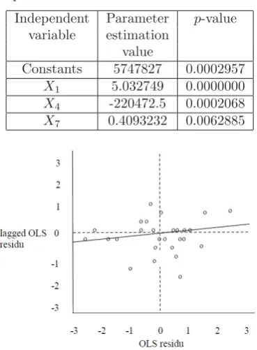
[image:4.595.326.511.127.378.2]Yi= 5747827+5.032749X1i−220472.5X4i+0.4093232X7i with valueR2was 0.994140. It means that 99.4 % paddy production in Indonesia in 2011 could be explained by the paddy harvested area, average monthly temperature and numbers of farming workers in sub sector food plan-tation. Meanwhile, the rest at 0.586 % was explained by other unobserved factors in this study. In the en-tire test on the best regression model, it was obtained the value of 4.5515×10⁻³³ < α= 0.05; thus, it can be concluded that at least there was one regression para-meter significantly influential for the paddy production in Indonesia in 2011. The values of parameter estimation and p-value to each parameter could be observed in Ta-ble 1. As seen in TaTa-ble 1, three parameters in regression model have a significant influence because each ofp-value < α= 0.05. Then, regression assumption model testing was done with the result showing the fulfilled normal-ity, homogeneity and non multi collinearity assumptions.
Table 1: Parameter estimation value andp-value to each parameter
Independent Parameter p-value variable estimation
value
Constants 5747827 0.0002957 X1 5.032749 0.0000000
X4 -220472.5 0.0002068
X7 0.4093232 0.0062885
Figure 1: Scatter Diagram of Moran Index for Paddy Production
However, error on closed-relation area may connect or was spatially correlated. The indicators of any auto spa-tial correlation effects could be observed from Moran in-dex in scatter diagram as seen in Figure 1. Diagonal lines were closed to zero, meaning no spatial autocorrelation in the model by using spatial regression model. Further-more, steps to construct spatial regression model were conducted by testing spatial effects with Lagrange multi-plier, maximum likelihood estimation, parameter signifi-cance testing, assumptions testing.
4.1
Lag Spatial Model
The Moran’s scatter diagram can only be applied to iden-tify the existence of spatial autocorrelation in a certain area but cannot discover spatial autocorrelation in model. Hence Lagrange lag and error testing were highly needed. The Lagrange lag multiplier testing included:
1. H0: there was no lag spatial dependency (ρ= 0) H1: there was lag spatial dependency (ρ= 0).
2. Significance level (α) = 0.05.
3. Critical area
H0 was rejected ifLMp> χ2(0.05,1) = 3.841.
4. Statistic value,LMp= 5.3173358.
5. Conclusion
Since LMp = 5.3173358 > 3.841 so we concluded
IAENG International Journal of Applied Mathematics, 45:4, IJAM_45_4_19
that H0 was rejected meaning that there was lag spatial dependency in the model.
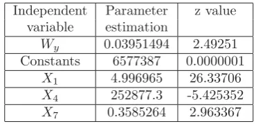
Therefore, regression model had spatial autocorrelation in lag; thus, it could be presented with lag spatial re-gression model. The value of parameter estimation of lag spatial regression model and z could be calculated as seen in Table 2. Model of lag spatial discussed can be seen as follows:
Y =0.03951494Wy+ 4.996965X1−252877.3X4
+ 0.3585264X7. (5)
[image:5.595.68.255.301.391.2]Based on Table 2 it could be seen that absolute value of z
Table 2: Parameter estimation value and z value calculated in lag spatial regression model
Independent Parameter z value variable estimation
Wy 0.03951494 2.49251 Constants 6577387 0.0000001
X1 4.996965 26.33706
X4 252877.3 -5.425352
X7 0.3585264 2.963367
calculated in each independent variable was greater than z0.025= 1.96; thus, it can be concluded that paddy har-vested area, average monthly temperature and numbers of farming workers in sub sector food plantation had sig-nificant influence on Indonesia paddy production in 2011. After obtaining the estimation of parameter model, the significance testing of parameter model was conducted using likelihood ratio testing that included:
1. H0: ρ = 0 (spatial parameter was not significantly influenced)
H1: ρ= 0 (spatial parameter was significantly
influ-enced).
2. Significance level (α) = 0.05.
3. Critical area
H0 was rejected ifLRTρ > χ2(0.05,4) = 3.841.
4. Statistic value,LRTρ= 5.716419.
5. Conclusion
Since LRTρ = 5.716419 > 3.841, it could be con-cluded thatH0was rejected meaning that lag spatial parameter was significantly influenced.
Furthermore, homoscedastic testing was conducted to de-termine whether a spatial lag regression models met the assumptions. Homoscedastic test performed by Breusch-Pagan could be seen as follows:
1. H0: There was no heteroscedasticityH1: There was heteroscedasticity
2. Significance level (α) = 0.05.
3. Critical area
H0 was rejected ifBP > χ2(0.05,2)= 9.488.
4. Statistic value,BP = 1.453798.
5. Conclusion
Since BP= 1.453798<9.488, it then could be con-cluded thatH0 was not rejected meaning that there was no heteroscedasticity in the model.
4.2
Error Spatial Model
The initial step in presenting error spatial model of In-donesia paddy production data in 2011 is Lagrange mul-tiplier testing:
1. H0: λ= 0 (spatial parameter was not significantly influenced)
H1: λ= 0 (spatial parameter was significantly
influ-enced).
2. Significance level (α) = 0.05.
3. Critical area
H0 was rejected ifLRTλ> χ2(0.05,4)= 3.841.
4. Statistic value,LRTλ= 0.2367617.
5. Conclusion
Since LRTλ = 0.2367617 <3.841, it could be con-cluded thatH0was not rejected meaning that error spatial parameter was not significantly influenced.
Based on Lagrange error multiplier testing, it could be concluded that this model did not have any spatial auto-correlation in error. Thus, given lag spatial dependency and no error spatial dependency causes Indonesia paddy production in 2011 could be presented as lag spatial re-gression model. Model (5) shows that an increase of one hectare of paddy harvested area would increase paddy production as 4.996965 tons. Each increasing of 10C aver-age monthly temperature would reduce paddy production as 252877.3 tons and each of increase of one agricultural labor in food crop sub sector would increase paddy pro-duction as 0.3585264 ton. Spatial autocorrelation at lag in the model (5) is shown by the spatial lag parameter value of 0.03951494.
Based on lag spatial model, paddy production in all provinces was estimated so the production map in In-donesia could be created (Figure 2). There are 21 provinces that are included in the low category and 9 provinces included in the moderate category. Provinces with highest paddy production are Central Java, East Java and West Java.
IAENG International Journal of Applied Mathematics, 45:4, IJAM_45_4_19
Figure 2: Prediction of Paddy Production in Indonesia
References
[1] Anselin, L., Spatial Econometrics: Methods and Models, Kluwer Academic Press, London, 1988.
[2] Badan Pusat Statistik, Production of Paddy, Maizze, and Soybeans, www.bps.go.id/releases/ Pro-duction of Paddy Maizze and Soybeans, 2012.
[3] Lee, J., and Wong, D.W.S,Statistical Analysis with ArcView GIS, John Wiley and Sons, Inc., New York, 2001.
[4] Lesage, J.P., The Theory and Practice of Spatial Econometrics, Dept. of Economics, University of Toledo, Ohio, 1999.
[5] Susanti, Y. and Pratiwi, H., Robust Regression Model for Predicting the Soybean Production in In-donesia, Canadian Journal on Scientific and Indus-trial Research, Vol. 2, No. 9, pp. 318-328, 2001.
[6] Yohai, V.J., High Breakdown Point and High Effi-ciency Robust Estimates for Regression,The Annals of Statistics, Vol. 15, No. 20, pp. 642-656, 1987.
[7] Zhang, Z., Robust Estimations, http: //www.sop. Inria.tr/robust/personel/zzhang, 1996.