Automated Segmentation of Lumbar Vertebrae in
Digital Videofluoroscopic Images
Yalin Zheng*, Mark S. Nixon, and Robert Allen
Abstract—Low back pain is a significant problem in the industrialized world. Diagnosis of the underlying causes can be extremely difficult. Since mechanical factors often play an important role, it can be helpful to study the motion of the spine. Digital videofluoroscopy has been developed for this study and it can provide image sequences with many frames, but which often suffer due to noise, exacerbated by the very low radiation dosage. Thus, determining vertebra position within the image sequence presents a considerable challenge.
There have been many studies on vertebral image extraction, but problems of repeatability, occlusion and out-of-plane motion per-sist. In this paper, we show how the Hough transform (HT) can be used to solve these problems. Here, Fourier descriptors were used to describe the vertebral body shape. This description was incor-porated within our HT algorithm from which we can obtain affine transform parameters, i.e., scale, rotation and center position. The method has been applied to images of a calibration model and to images from two sequences of moving human lumbar spines. The results show promise and potential for object extraction from poor quality images and that models of spinal movement can indeed be derived for clinical application.
Index Terms—Low back pain, videofluoroscopy, Hough trans-form, Fourier descriptors, lumbar spine.
I. INTRODUCTION
T
HE spine constitutes the central axis of the body and con-sequently is a very important three-dimensional (3-D) me-chanical structure. It maintains several vital functions for the human body. It can support the weight of the trunk, transfer the weight to the pelvis, provide a wide range of mobility and provide necessary shock-absorbing resilience as well as protect the spinal cord from damage. The spinal column is described in terms of the cervical, thoracic, lumbar spine and sacroiliac regions. The lumbar spine is especially “designed” to bear con-siderable loads and to provide a large range of mobility. The spinal column system also includes ligaments and muscles. The ligaments take tensile loads and the muscles supply forces to maintain spine stability [1].Manuscript received October 1, 2002; revised June 7, 2003. The Associate Editor responsible for coordinating the review of this paper and recommending its publication was P. Cinquin.Asterisk indicates corresponding author.
*Y. Zheng was with the Electronics and Computer Science Department, Uni-versity of Southampton SO17 1BJ Southampton, U.K. He is now with the Com-putational Imaging Science Group, Division of Imaging Sciences, Guy’s, King’s and St. Thomas’ School of Medicine, King’s College London, London SE1 9RT, U.K. (e-mail: yalin.zheng@kcl.ac.uk).
M. S. Nixon is with the Electronics and Computer Science Depart-ment, University of Southampton, Southampton, SO17 1BJ, U.K. (e-mail: msn@ecs.soton.ac.uk).
R. Allen is with the Institute of Sound and Vibration Research, University of Southampton, Southampton SO17 1BJ, U.K. (e-mail: ra@soton.ac.uk).
Digital Object Identifier 10.1109/TMI.2003.819927
Analysis of the movement of the spine can be helpful in clin-ical diagnosis of low back pain (LBP). We shall first describe the basis of our work, the goals and their problems. Then we shall describe appropriate image modalities, highlighting that radio-graphic approaches compromise between image quality and ra-diation dosage. As this compromise often results in images of low quality, manual detection of landmarks (the currently fa-vored practice) can be difficult. In contrast, computer vision of-fers feature extraction techniques which are here shown to good effect by providing automated spinal analysis at what appears to be a reasonable level.
A. Spinal Problems
The low back is the area between T12 (T means the th vertebra of thoracic spine while L means the th vertebra of Lumbar Spine) and the hips [2]. LBP is defined as pain per-ceived as arising from either the lumbar spine or the sacroiliac region, or from a combination of both [3]. Its differential diag-nosis is complicated by its origin from multiple diseases and disorders [2]. Furthermore, understanding is also limited by the structural complexity of the spine and the difficulty of under-takingin vivodiagnosis and testing.
Humans have struggled against backache for many years [4]. LBP has been (and continues to be) one of the enigmas in modern medicine even though considerable technical advances have been made in diagnosis, treatment and rehabilitation. Both the problem and its associated disability have appeared to escalate with time [5]. Back pain is the second most common reason for a clinical visit [6].
There are, as yet, no well-accepted standards to determine the causes of LBP. Some studies tend to classify LBP as specific and nonspecific [7]. The latter are also called “mechanical low back problems.” As the cause of pain is biomechanical in nature whist the pain may also cause abnormal motion, many attempts have been made to establish the relationships between motion and LBP [8]. Mechanical disorders can be described by joint kinematics and knowledge of the forces acting on the structures involved. As the forces are difficult to measurein vivo, clinical studies of spinal biomechanics primarily focus on joint kine-matics.
An important mechanical cause of LBP is spinal instability and, indeed, might be one of the most common causes. It is esti-mated that 20%–30% of LBP patients have spinal instability [9]. Controversy surrounds the word “instability” when describing potential causes of LBP [8], particularly since hypermobility is seen in many patients who have little or no pain. Similarly, many patients presenting with LBP have no demonstrable instability
[10]. Links between potentially painful spinal pathology and ab-normal spinal movements may then help clinicians to formulate and evaluate their own definition of spinal instability [11]. Char-acterising spinal motion is, however, extremely difficult. There-fore, study of spinal movement could help in its definition and may benefit diagnosis and clinical surgery.
Despite the large number of studies, the relationship between motion and LBP is still uncertain. For example, a dynamic mo-tion study failed to find a significant difference between chronic LBP patients and normal volunteers during actual movement [12]. However, this study did show that segmental instability in-fluences the whole lumbar motion in patients with degenerative spondylolisthesis.
In correspondence to the large number of spinal motion analyses, different parameters are used to describe the kine-matics, i.e., intervertebral angles, sagittal translation, neutral zone, range of motion, etc. [13]. Pearcy and Bogduk also used the centrode (the loci of the instantaneous center of rotation (ICR) which is also often used) to describe the motion, but suggested that this is unable to distinguish normal or abnormal motion particularly for LBP patients with restricted movement because in these cases the centrodes may be subject to large errors [14].
B. Digital Videofluoroscopic (DVF) Imaging Technique
Imaging techniques have been widely used to capture the spinal motion information. However, plain X-rays, computer-ized tomography (CT), and magnetic resonance imaging (MRI) appear impractical to record continuous spinal motion. Plain X-ray radiography is widely used in medicine, but due to the high radiation dosage only a limited number of static images is obtained, usually in the neutral position and at the extreme positions of mobility. Consequently, it is not possible to deter-mine the intermediate states or to describe motion as the spine moves. Although bi-planar X-rays have the potential to obtain information on 3-D spinal motion [15], they encounter the same radiation risk problem as plain X-rays.
CT can usually provide images with good quality [16]. It re-quires the patient to be as stationary as possible for every scan, and it will also significantly raise radiation risk to the patients when a large number of scans are required. CT cannot, at least now, be suitable for the continuous spinal motion study. MRI can acquire very clear and accurate images (particularly of soft tissue) without radiation risk, but it is not yet fast enough for mo-tion analysis [17]. Furthermore, it increases the cost of diagnosis for persistent LBP and has even been considered as an add-on rather than a substitute for other imaging modalities in the eval-uation of persistent LBP [18]. Ultrasound is a safe and noninva-sive imaging technique, but unfortunately the images are not yet of sufficient quality to allow detailed investigation of the spinal column in motion.
[image:2.612.370.482.63.148.2]To overcome the problem of recording the continuous spinal motion, a DVF imaging technique, was first introduced by Breen and Allen et al. in 1987 [19] and has undergone considerable development since that time [20]–[23]. With this technique, a series of dynamic frames of spinal motion can be captured with a lower X-ray dosage than that required for a single plain X-ray plate of the lumbar spine. A typical DVF
Fig. 1. Lateral DVF image of the lumbar spine.
image of the lumbar spine is shown in Fig. 1. This was obtained from a study of passive motion in which the subject lay on an articulated table and was moved passively at a controlled rate.
C. Previous Landmark Locating Methods
When the radiographic images have been acquired, certain points (anatomical marks) on the vertebra within the image have to be located in order to determine the parameters of the motion and this procedure is called landmark identification. Landmark location is the core of the study and the accuracy of the estimated kinematics greatly depends on this procedure. Without accuracy in landmarking, it is impossible to determine kinematic parame-ters correctly. Originally, this work was manual and consisted of locating the corners of the vertebrae as anatomical landmarks. However, this procedure was inevitably affected by many fac-tors. It is difficult to place markers exactly on the vertebral cor-ners and furthermore, repeatability cannot be assured. Panjabiet al.discussed in detail errors that arise when manually marking X-ray images of the spine [24].
Several approaches based on correlation have been proposed to overcome these problems. Simoniset al.[21] used a template matching method wherein the template comprised the whole vertebral body. Muggleton and Allen [22] obtained some im-provements by using an annular template containing the margins of the vertebra. Recently Cardan and Allen [23] proposed a first pixel algorithm to increase computational speed but this was still based on a template matching method, which may suffer when out-of-plane motion is evident or when occlusion occurs.
Other computer vision techniques have also been applied to vertebra extraction and might have potential to improve land-mark location. Hamadehet al.[25] proposed a solution to esti-mate the motion based on 3-D/two-dimensional (2-D) registra-tion of 3-D surface models obtained from CT slices with 2-D X-ray images. The method itself might be useful but the system is very complex and is time consuming. Smythet al.[26] used an active shape mode, which is generated by principal components analysis. This improves robustness by using shape constraints, but requires training data before it can be implemented. Brejlet al.[27] proposed a method of automated segmentation of ver-tebrae in MRI images but this study also needs training data.
technique to provide more accurate, reliable and robust land-marks. The paper is organized as follows: Section II introduces the Hough transform (HT) approach used in the current study; Section III reports the extraction results from a synthetic image, from a calibration model with two vertebrae and from DVF images also assessing performance of the HT in occlusion and noise. Section IV shows the new potential to describe the motion pattern and presents some useful discussions which are concluded in Section V and future directions suggested.
II. THEHOUGHTRANSFORMALGORITHM
The HT was first introduced by Hough [28] and has become one of the most popular tools in computer vision because of its robustness. It has been applied to a wide variety of problems in machine vision, e.g., line detection [28], [29], circle detec-tion [30], arbitrary shape extracdetec-tion [31]–[33], and modetec-tion ex-traction [34]. There are two comprehensive reviews of the HT [35], [36]. Although there have been some valuable analyses of its performance, there has been no consistent definition of the transform itself. Amongst these definitions, Aguadoet al.[37] gave the most elegant definition of the HT based on the principle of duality. Sklansky [38] showed that the HT provides a result equivalent to that derived by template matching but with less computational effort. The HT, thus, inherits advantages such as immunity to noise and occlusion.
A. The Generalized Hough Transform (GHT)
[image:3.612.362.499.378.509.2]The HT for arbitrary shape extraction is similar to an original form [31] that aimed to determine the position of a reference point indicating a shape’s, or a target contour’s, position. For a given edge point in an image and target contour, the possible loci of positions of the reference point is the curve obtained by rotating the target curve by 180 (centered at that edge point). By repeating this procedure for all edge points, more possible reference point loci can be obtained. The position of the refer-ence point is selected as the point which has the maximal in-tersections of these loci. In implementation, the ranges of the unknown parameters are converted into an array by quantising them in order to store the coordinates of the intersection points. This array is called the accumulator space (or parameter space). However, the original form is not well-developed because it does not provide an efficient way to describe the arbitrary shape, which is the key element in this method. The GHT [32] uses edge information to define a mapping from the orientation of an edge point to a reference point of the shape. The template shape is represented by an R-table, which is a discrete lookup table. When the template is scaled or rotated, there can be prob-lems with aliasing and rounding. Distortions are inevitable when working with discrete representations. Nevertheless, the worst effects can be avoided by maintaining a continuous representa-tion for as much of the process as possible.
B. Adaption of the GHT With Fourier Descriptors
In an adaptation of the GHT [33], elliptic Fourier descriptors are used to describe the shape. This representation gives a continuous representation that can be sampled at any resolution without the aliasing problems of the R-table. Elliptic Fourier
descriptors are chosen for their completeness, simple geometric interpretation, access to frequency information and the fact that they can be easily produced from a chain code of the model contour [39]. However, other analytic representations (e.g., wavelets) might equally be used.
1) Fourier Description of a Shape: A 2-D curve can be mathematically described by a vector function, which defines the positions of the points along it by their components in two orthonormal axes. That is
(1)
where and are two orthonormal
vectors.
According to Fourier theory, and can be expressed by Fourier expansion. That is
(2)
In (2), defines the angular frequency and is the harmonic number. The coefficients , and , which are later called Fourier descriptors (FDs), can be computed by the dis-crete approximation given in trigonometric form as
and
and
(3)
where is the number of sampling points and and repre-sent the position of point in the model shape.
Thus, (2) can be expressed in matrix form as
(4)
Given the discrete nature, the possible number of frequencies in the expansion should be integers between 1 and as suggested in sampling theory, but the determination of the max-imal frequency still deserves some discussion especially when the sampling points are very few and the curve has very sharp corners. For convenience, the DC components and in (4) can be omitted since any curve can be defined with its center at the origin of the coordinate system. That is
(5)
2) Hough Algorithm: Any curve obtained by applying an affine transformation (only translation, scaling and rotation are considered here, shears should be included as well.), can be ex-pressed by its two components in the and directions. That is
(6)
where represents scale, is the clockwise rotation, and , are translations in the and directions.
Following the derivation of the HT [33], we define the trans-formation kernel as
(7)
For any edge point obtained by edge detection, we can obtain its translation vector
(8)
As introduced earlier, in order to form the accumulator array an evaluation criterion has to be made in order to increase the values of the array cells where there are intersections. Here, a simple matching function is defined as
(9)
Where, and can be vectors. We can now define the HT in discrete form as
(10)
where is the translation vector, and is a four-dimensional (4-D) accumulator array which stores the number of intersections. defines the edge points found in the image and is the domain of the points in the model shape.
Thus, the real translation vector , rotation , and scale can be obtained by locating the maximal value in (10), where
. That is
(11)
The expression of (11) that defines the HT using FDs for arbi-trary shape extraction is used in the present work. Essentially, for a given feature point, a locus of points is plotted through the 4-D (translation in the and directions, rotation and scale .) accumulator space. This locus is formed from scaled and ro-tated representations of the model in 2-D planes along the and
axis of the accumulator space.
III. RESULTS
A. Example Extraction
First, the HT was applied to a simple synthetic image, shown in Fig. 2. Its width and height are 126 and 115 pixels respectively and the center of the target object mathematically is located at (60.75, 55.26), which can be rounded to the nearest pixel posi-tion (61, 55). The true results should be
[image:4.612.309.539.67.202.2], and . The total number of edge points is 377. The FDs were obtained from the chain code of the contour [39]. Fig. 3 shows the reconstructions with different number
Fig. 2. Original curve.
Fig. 3. Reconstruction with different FDs. (a) Four FDs, (b) eight FDs, (c) 16 FDs, and (d) 32 FDs.
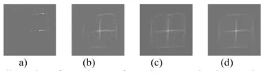
Fig. 4. Illustration of Hough space formation. (a) One point, (b) 50 points, (c) 100 points, and (d) 377 points (total).
of FDs. With more harmonics, the reconstruction is increas-ingly close to the original shape. Notice that the total harmonics should conform to sampling theory, as mentioned earlier.
As discussed above, the core of the HT is forming the accu-mulator space. In this experiment, the ranges of scale, rotation, , and are 1 to 5, 5 to 5, 0 to 125, and 0 to 114, respec-tively. By assuming resolutions for scale, rotation and transla-tion are unity, 1 and one pixel, respectively, a 4-D accumulator array with the size of 5 11 126 115 can be constructed by quantising the ranges of these parameters into intervals. As introduced earlier, each edge point votes in this array. That is, if the parameters obtained are within the range set earlier, the value of the corresponding cell will be increased by one. In this way, the array is assigned value by all the edge points. Then the parameters can be determined by locating the array maximum. To illustrate this procedure, we transform array values into the image (for convenience, only the vote distribution for transla-tion is shown with scale of unity and rotatransla-tion of 0 ), in which the brightness of accumulator points is proportional to the number of votes they obtained. Here, 16 FDs are used. In Fig. 4, from left to right, are the Hough space formed by 1, 50, 100, and 377 edge points. The position of the brightest point is the values of
and we are looking for. In Fig. 4(d), the coordinate of the brightest point is (61, 55) and this means that the and parameter values are (61, 55) as expected.
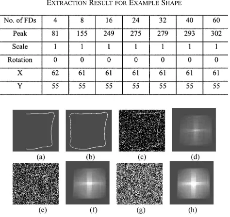
[image:4.612.333.527.242.297.2]TABLE I
[image:5.612.46.283.76.300.2]EXTRACTIONRESULT FOREXAMPLESHAPE
Fig. 5. (a) Twenty-five percent occlusion and different noise levels, (b) extraction result, (c) 30% noise, (d) Hough space (30% noise, (e) 60% noise, (f) Hough space (60% noise), (g) 85% noise, and (h) Hough space (85% noise).
no improvement over that by 16 descriptors and the vote values only increase slightly. Clearly, the results of 16 descriptors are sufficient for a more refined analysis of the match at the verte-bral corners, which is the main objective of this approach.
B. Noise and Occlusion
Another concern is to what degree the HT can resist occlu-sion and noise. We considered instances of the whole shape, 25% and 75% occlusion with different noise levels from 0% to 95%. In this test, 16 FDs were used. As in practice it is difficult to exactly determine the noise in real images, here we examine the performance of the HT by adding “salt and pepper” noise to the edge image. Occlusion is simulated by removing certain chosen parts from the edge image. Fig. 5 shows 25% occlusion, its results and images with different noise levels and the corre-sponding Hough spaces. In the Hough space images, the relative bright area spreads with the increase in noise level. This means that the signal-to-noise ratio decreases and the peak is gradu-ally impaired and eventugradu-ally inundated by the peaks generated by noise.
Visually when the noise level is about 60%, the shape cannot be identified by human vision. The results show that the HT can work well until the noise level is 90% for the whole shape. When there is occlusion, this ability has a slight reduction. It can succeed until the noise levels are 85% and 70% for 25% and 75% occlusion, respectively. Fig. 6 shows 75% occlusion and its extraction results.
These results confirm that the HT has a good ability to resist noise and occlusion, and can be useful for application to medical images.
C. Application to Calibration Model
When a clinical measuring technique is developed, it is essen-tial to demonstrate its reliability before it can be used in clinical
[image:5.612.304.514.227.386.2]Fig. 6. (a) Seventy-five percent occlusion and different noise levels, (b) extraction result, (c) 30% noise, (d) Hough space (30% noise), (e) 60% noise, (f) Hough space (60% noise), (g) 70% noise, and (h) Hough space (70% noise).
Fig. 7. Calibration model.
Fig. 8. L4 model and edge image of one frame (by Sobel Operator). (a) L4 model and (b) edge image
trials. In our study, we test it by measuring the motion parame-ters that can be preset in a calibration model, shown in Fig. 7.
The calibration model is comprised of two human lumbar ver-tebrae (L3 and L4) linked at the position of the centrum of the disc by means of a universal joint. A perspex pointer was fitted to the front of the body of the superior vertebra in such a way as to describe arcs whose centers corresponded to the universal joint. A CNC machine tool was used to preset the angular posi-tion in 2-D. The measurement of these arcs was obtained from a protractor attached to the base of the model. The increment of the preset angles is 5 and the useful range of this protractor was 30 .
Fig. 8 shows the L4 model and edge information of one frame. Table II shows the extraction results with 16 FDs. A series of results over a range of intervertebral angles are shown in Fig. 9. The value shown on the top right of each frame is the preset rotation angle of L3. The negative value means that motion is in the flexion direction and positive means extension.
D. Application to an In Vivo Image Sequence
TABLE II
[image:6.612.47.284.84.264.2]THEEXTRACTIONRESULTS OFCALIBRATIONMODEL
[image:6.612.365.500.175.395.2] [image:6.612.57.272.273.376.2]Fig. 9. Extraction results of the calibration model.
Fig. 10. L3 (in Frame 1) image, edge, and results with 16 FDs.
Fig. 11. Extraction results in DVF images of sequence one.
Fig. 10 shows the extraction of the L3 in frame one of a motion sequence. Fig. 11 shows the results in different frames of one sequence and Fig. 12 shows results on two DVF frames of an-other subject.
[image:6.612.53.277.413.478.2]Fig. 12. Extraction results in DVF images of sequence 2.
Fig. 13. Vertebral center connection of the lumbar spine in a sequence.
IV. DISCUSSION
Much information about the spinal motion can be obtained from the above results. For example, how the vertebral centers move in a motion sequence can be determined. Fig. 13 shows such change during five frames of a sequence. From top to bottom, the symbols represent the centers of the lumbar verte-brae from L1 to L5, and these move across the image frames. L5 moves the largest distance while L1 hardly changes posi-tion. This is consistent with the passive movement of the subject due to the constraints that impede motion of L1. Similarly, other parameters such as rotation angles and translations can also be obtained by simple calculation. In short, the HT can become a powerful method to acquire the data needed for kinematic anal-ysis of the lumbar spine.
The required accuracy for clinical analysis is likely to be 1 –2 [40]. However, current manual labeling approaches are tedious and error prone and not able to quantify motions but only at the end points of the motion. Accuracy problems are really in detecting landmarks since these can affect kinematic indexes such as the ICR—the small errors in the landmarking lead to large errors in ICR.
[image:6.612.62.271.516.672.2]PC with 256 M memory. It would be much faster by rewriting in C and optimising the code. We have to note that, however, it is unnecessary to analyze the motion sequence in real time in clinical application. Moreover, the motion sequence can be pro-cessed by parallel computation to save time.
One concern is the model of the vertebral contour. As we know, the vertebral endplates have nonsharp edges and the pro-jection of them on the sagittal plane may become fuzzy and may not be constant throughout the motion sequence. However, this just suggests why the HT has an advantage over the ear-lier manual methods from another aspect. As discussed earear-lier, the HT can locate the vertebrae by collecting evidence over the whole contour rather than at several corner points and, thus, it will not be seriously affected by partial deformation, missing data, or inconsistent changes of the image illumination. In con-trast, manual marking is difficult or impossible to cope with such cases. Although the end-plate shape sometimes can be very helpful in diagnosing disease, as our main focus is the motion rather than exact shape of the end-plate, we do not think it is vital in this study.
In addition, due to the coupling within spinal motion, the out-of-plane motion has been studied. It has been widely accepted that the coupled axial rotation is small during the flexion/extension in the sagittal plane and, thus, in practice it has often been neglected [11]. Moreover, during the DVF acquisition in the current study, the subject is lying on a passive motion table and this will further constrain the out-of-plane motion. Therefore, it appears reasonable for us to assume that the flexion/extension is limited to 2-D. In clinical practice, where spontaneous bending movements may be made by the patient, the out-of-plane motion problem is increased. Even with a restraint placed around the hips, for example, it is likely to be difficult to properly constrain the motion to 2-D. An objective is, however, to extend the technique into 3-D. Theo-retically, the HT has the ability to cope with the out-of-motion problem which can be regarded as 3-D object identification [41]. However, it is likely to be more complex and, therefore, computationally expensive as more parameters are involved.
Finally, although currently DVF is the only practical means to acquire motion sequences, the appearance of better image modalities in the future cannot be ruled out. For example, a pro-totype 4-D CT scanner has been proposed [42]. Even as new imaging techniques develop, our method should still work well as a generic tool since the new techniques are likely to offer im-provements in image quality.
V. CONCLUSIONS ANDFUTUREWORK
Vertebral extraction from DVF images has been a popular goal for a considerable time. However, this has been proved to be very difficult due to the poor image quality. Vertebral extraction is an image processing problem and consequently, algorithms from the field of computer vision could have a valuable role to play. The HT has many desirable properties, especially good resistance against noise and occlusion, and hence might be suit-able for coping with the problems inherent with DVF images.
In this paper, the theory of the arbitrary HT was first intro-duced. Then the effects of different FDs, noise, and occlusion on
the final extraction were investigated. It also provided encour-aging results when used on a calibration model. Finally, it was applied toin vivoDVF lumbar spine images and gave promising results. The great advantage of the HT is that it can locate the same vertebral contour in the sequences and, thus, contour shape will not change, which is important when the vertebral image suffers noise or occlusion. Furthermore, many kinematic param-eters can be obtained based on the HT. In this paper, we only show the changing pattern of the lumbar spine vertebral centers. This could provide clinicians with valuable information for di-agnosis of spinal disorders.
In DVF images, it is possible to observe that the image quality of the L5 area is very poor. Sometimes, L5 cannot easily be discerned by eye. Although our method can obtain satisfactory results for some DVF images, sometimes it might fail in ex-traction. Therefore, there is still effort needed to improve the method in order to cope with this problem. In fact, the present method only considers the vertebrae separately. As we know that there are some intrinsic relationships between the verte-brae, for example, the distance of the neighboring segments should not change greatly and the motion parameters should not change abruptly. At present, a new version of the HT called the spatio-temporal HT is being developed. This combines the HT with spatial and temporal information and is particularly attrac-tive for coping with medical image sequences of poor quality.
ACKNOWLEDGMENT
The authors wish to thank the Anglo-European College of Chiropractic (AECC), and particularly Dr. M. Kondracki, for kindly providing the DVF image sequences. Y. Zheng grate-fully acknowledges tenure of a research studentship supported by Faculty of Engineering and Applied Science at the University of Southampton. The reviewers’ input is gratefully acknowl-edged.
REFERENCES
[1] K. Case, D. C. Xiao, B. S. Acar, and J. M. Porter, “Computer aided modeling of the human spine,” inProc. Inst. Mech. Engrs., vol. 213, 1999, pp. 83–86.
[2] Low Back Pain Handbook, Butterworth and Heinemann, Boston, MA, 1999.
[3] N. Bogduk,Clinical Anatomy of the Lumbar Spine and Sacrum, London, U.K.: Churchill Livingston, 1997.
[4] D. B. Allan and G. Waddell, “An historical perspective on low back pain and disability,”Acta Orthop Scand, vol. 60, pp. 1–23, 1989.
[5] J. A. Porterfield and C. Derosa,Mechanical Low Back Pain: Perspective in Functional Anatomy, 2nd ed. Philadelphia, PA: Saunders, 1998. [6] North American Spine SocietyFacts About Back Pain [Online].
Avail-able: http://www.spine.org/bthw/FactsAboutBackPain.htm
[7] M. W. Tulder, W. J. J. Assendelft, B. W. Koes, and L. M. Bouter, “Spinal radiographic findings and nonspecific low back pain,”Spine, vol. 22, no. 4, pp. 427–434, 1997.
[8] M. Szpalski, R. Gunzburg, and M. H. Pope,Lumbar Segmental Insta-bility. Philadelphia, PA: Lippincott Williams & Wilkins, 1999. [9] M. H. Pope and M. Panjabi, “Biomechanical definitions of spinal
insta-bility,”Spine, vol. 10, pp. 255–256, 1985.
[10] S. M. Eisenstein, “‘Instability’ and low back pain a way out of the maze,” inLumbar Segmental Instability. Philadelphia, PA: Lippincott Williams & Wilkins, 1999.
[12] A. Okawa, K. Shinomiya, H. Komori, T. Muneta, Y. Arai, and O. Nakai, “Dynamic motion study of the whole lumbar spine by videoflu-oroscopy,”Spine, vol. 23, no. 16, pp. 1743–1749, 1998.
[13] J. M. Muggleton and R. Allen, “Insight into the measurement of ver-tebral translation in the sagittal plane,”Med. Eng. Phys., vol. 20, pp. 21–32, 1998.
[14] M. J. Pearcy and N. Bogduk, “Instantaneous axes of rotation of the lumbar intervertebral joints,”Spine, vol. 13, no. 9, pp. 1033–1041, 1988. [15] M. Mimura, “Rotational instability of the lumbar spine—A three-dimen-sional motion study using Bi-plane X-ray analysis system,”Jpn. Or-thopaedics Assoc., vol. 64, pp. 546–559, 1990.
[16] J. Beutel, H. L. Kundel, and R. L. Van Metter,Handbook of Medical Imaging. Bellingham, WA: SPIE, 2002, vol. 1, Physics and Psy-chophysics.
[17] Z. H. Cho, J. P. Jones, and M. Singh, Foundations of Medical Imaging. New York: Wiley, 1993.
[18] S. J. Ackerman, E. P. Steinberg, R. N. Bryan, M. BenDebba, and D. M. Long, “Trends in diagnostic imaging for low back pain: Has MR imaging been a substitute or add-on?,”Radiation, vol. 203, no. 2, pp. 533–538, 1997.
[19] A. C. Breen, R. Allen, and A. Morris, “A computer/X-ray method for measuring spinal segmental movement: A feasibility study,”Trans. Pa-cific Consortium Chiropractic Res., pp. E.31–E.37, 1987.
[20] A. Breen, R. Allen, and A. Morris, “A digital videofluoroscopic tech-nique for spine kinematics,”J. Med. Eng. Technol., vol. 13, no. 1/2, pp. 109–113, 1989.
[21] C. Simonis and R. Allen, “Calculation of planar spine kinematic param-eters using videofluoroscopic images and parallel processing,” inProc. 15th IEEE Engineering in Medicine and Biology Society, San Diego, CA, Oct. 28–31, 1993, pp. 1087–1088.
[22] J. M. Muggleton and R. Allen, “Automatic location of vertebrae in dig-itized videofluoroscopic images of the lumbar spine,”Med. Eng. Phys., vol. 19, pp. 77–89, 1997.
[23] C. Cardan and R. Allen, “Measurement of spine motion for diagnosis of mechanical problems,”J. Simulation Modeling Med., vol. 1, no. 1, pp. 15–19, 2000.
[24] M. Panjabi, D. Chang, and J. Dvo˘rák, “An analysis of errors in kinematic parameters associated within vivofunctional radiographs,”Spine, vol. 17, no. 2, pp. 200–205, 1992.
[25] A. Hamadeh and P. Cinquin, “Kinematic study of lumbar spine using functional radiographies and 3D/2D registration,” in Lecture Notes in Computer Science. Berlin, Germany: Springer-Verlag, 1997, vol. 1205, pp. 109–128.
[26] P. P. Smyth, C. J. Taylor, and J. E. Adams, “Automatic measurement of vertebral shape using active shape models,”Image Vis. Computing, vol. 15, pp. 575–581, 1997.
[27] M. Brejl and M. Sonka, “Automated Initialization automated design of border detection criteria in edge-based segmentation,” inProc. 4th IEEE Southwest Symp. Image Analysis and Interpretation, TX, 2000, pp. 26–30.
[28] P. V. C. Hough, “A Method and Means for Recognizing Complex Pat-terns,”, 1962.
[29] R. O. Duda and E. Hart, “Use of the Hough transform to detect lines and curves in pictures,”Commun. ACM, vol. 15, no. 1, pp. 11–15, 1972. [30] C. Kimme, D. Ballard, and J. Sklansky, “Finding circles by an array of
accumulators,”Commun. ACM, vol. 18, pp. 120–122, 1975.
[31] P. M. Merlin and D. J. Farber, “A parallel mechanism for detecting curves in pictures,”IEEE Trans. Comput., vol. C-24, pp. 96–98, 1975. [32] D. H. Ballard, “Generalizing the Hough transform to detect arbitrary
shapes,”Pattern Recogn., vol. 13, no. 2, pp. 111–122, 1981.
[33] A. S. Aguado, M. S. Nixon, and M. E. Montiel, “Parameterizing arbi-trary shapes via Fourier descriptors for evidence-gathering extraction,”
Comput. Vis. Image Understanding, vol. 69, pp. 202–221, 1998. [34] J. M. Nash, J. N. Carter, and M. S. Nixon, “Dynamic feature extraction
via the velocity Hough transform,”Pattern Recogn. Lett., vol. 18, pp. 1035–1047, 1997.
[35] J. Illingworth and J. Kittler, “A survey of the Hough transform,”Comput. Vis., Graphic., Image Understanding, vol. 44, pp. 87–116, 1988. [36] V. F. Leavers, “Survey: Which Hough transform?,”CVGIP: Image
Un-derstanding, vol. 58, no. 2, pp. 250–264, 1993.
[37] A. S. Aguado, E. Montiel, and M. S. Nixon, “On the intimate relationship between the principle of duality and the Hough transform,” inProc. Roy. Society—A, vol. 456, 1998, pp. 503–526.
[38] J. Sklansky, “On the Hough technique for curve detection,”IEEE Trans. Comput., vol. C-27, pp. 923–926, 1978.
[39] F. P. Kuhl and C. R. Giardina, “Elliptic Fourier features of a closed con-tour,”Comput. Graphic. Image Processing, vol. 18, pp. 236–258, 1982. [40] A. A. White and M. M. Panjabi,Clinical Biomechanics of the Spine, 2nd
ed. Philadelphia, PA: Lippincott-Raven, 1990, vol. 1.
[41] W. H. Lou and A. P. Reeves, “Three-dimensional generalized Hough transform for object identification,”Proc. SPIE, vol. 1192, Intelligent Robots and Computer Vision VIII: Algorithms and Techniques, pp. 363–374.