Land Suitability Evaluation for Agricultural Cropland in Mongolia Using the Spatial MCDM Method and AHP Based GIS

http://www.scirp.org/journal/gep ISSN Online: 2327-4344

ISSN Print: 2327-4336

DOI: 10.4236/gep.2017.59017 Sep. 26, 2017 238 Journal of Geoscience and Environment Protection

Land Suitability Evaluation for Agricultural

Cropland in Mongolia Using the Spatial MCDM

Method and AHP Based GIS

Munkhdulam Otgonbayar

, Clement Atzberger

, Jonathan Chambers

, D. Amarsaikhan

,

Sebastian Böck

, Jargaltulga Tsogtbayar

1_{Institute of Geography-Geoecology, Mongolian Academy of Sciences, Ulaanbaatar, Mongolia}

2_{Institute of Surveying, Remote Sensing and Land Information, Department of Landscape Spatial and Infrastructure Science,} University of Natural Resources and Life Sciences, Vienna, Austria

3_{Eng-Geo Tech LLC, Ulaanbaatar, Mongolia}

Abstract

The purpose of this study was to prepare a cropland suitability map of Mon-golia based on comprehensive landscape principles, including topography, soil properties, vegetation, climate and socio-economic factors. The primary goal was to create a more accurate map to estimate vegetation criteria (above ground biomass AGB), soil organic matter, soil texture, and the hydrothermal coefficient using Landsat 8 satellite imagery. The analysis used Landsat 8 im-agery from the 2016 summer season with a resolution of 30 meters, time series MODIS vegetation products (MOD13, MOD15, MOD17) averaged over 16 days from June to August 2000-2016, an SRTM DEM with a resolution of 30 meters, and a field survey of measured biomass and soil data. In total, 6 main factors were classified and quality evaluation criteria were developed for 17 criteria, each with 5 levels. In this research the spatial MCDM (multi-criteria decision-making) method and AHP based GIS were applied. This was devel-oped for each criteria layer’s value by multiplying parameters for each factor obtained from the pair comparison matrix by the weight addition, and by the suitable evaluation of several criteria factors affecting cropland. General accu-racy was 88%, while PLS and RF regressions were 82.3% and 92.8%, respec-tively.

Keywords

Land Suitability, MCDM, Boolean and Fuzzy Analysis, AHP, RF and PLS Regression

How to cite this paper: Otgonbayar, M., Atzberger, C., Chambers, J., Amarsaikhan, D., Böck, S. and Tsogtbayar, J. (2017) Land Suitability Evaluation for Agricultural Crop-land in Mongolia Using the Spatial MCDM Method and AHP Based GIS. Journal of Geoscience and Environment Protection, 5, 238-263.

https://doi.org/10.4236/gep.2017.59017

Received: August 15, 2017 Accepted: September 23, 2017 Published: September 26, 2017

Copyright © 2017 by authors and Scientific Research Publishing Inc. This work is licensed under the Creative Commons Attribution International License (CC BY 4.0).

DOI: 10.4236/gep.2017.59017 239 Journal of Geoscience and Environment Protection

1. Introduction

Science-based agricultural production has been developing intensively in

Mon-golia since 1960 [1]. Between 1960 and 1989 the total sown area increased from

267.1 to 846.1 thousand hectares. From 1989 the total sown area fell, reaching

165.0 thousand hectares in 2006 [2]. The sown areas rose steadily by 440.6

thou-sand hectares between the years 2006 and 2016. However, cropland remains 405.5 thousand hectares less than in 1989. In this same time period, the total population increased 3.19 times while the amount of sown area declined by half as compared with the population growth. There is a significant difference in vegetable consumption between the urban and rural population. Urban popula-tion vegetable consumppopula-tion is double that of the rural populapopula-tion [3].

In 1960, 40.2% of the total population lived in settled areas. This increased to 66.4% by 2016. Population increase coupled with consumption increase resulted in an intensified demand for food. On the other hand, agricultural products, es-pecially wheat and potato production, increased as a result of the national gov-ernment crop development program. Nowadays, potato and wheat consumption needs can be fulfilled by domestic production. However, of the total vegetable

consumption (not including potato), 40% - 45% were imported [4].

The main vegetables imports (onion, garlic, cabbage, turnips and other root seed vegetables) increased from 5438.4 tons in 1995 to 64,107 tons in 2016, an increase of 11.7 times. Of these, 96% - 99% were imported from China. Mongo-lia remains strongly dependent on food security from neighboring countries. In addition, soils of currently cultivated areas are degrading. The country is facing challenges (especially local governments and community groups) to identify new crop areas with enough capacity for cultivation.

We have previously studied this topic: “Land suitability evaluation for crop-land based on GIS between 2014 and 2016”, was funded by the Mongolian Agency of Administration of Land Affairs, Geodesy and Cartography. In our preliminary study we used small and medium scale digital thematic maps to analyze and assess land suitability for cropland. During the study it was recog-nized that there was a need to improve the accuracy of input data using high-resolution satellite imagery for future research [5].

Geographic information system (GIS) and remote sensing (RS) techniques have been broadly used in agricultural studies. Remote sensing can provide a timely and accurate picture of the agricultural sector, as it is very suitable for

gathering information over large areas with frequency and regularity [6]. The

derived information is used for qualitative and quantitative analysis within near real-time production forecasts as well as for the anticipation of food security

problems within the framework of monitoring agriculture [7].

2. Objectives

DOI: 10.4236/gep.2017.59017 240 Journal of Geoscience and Environment Protection

• _{Identify a methodology for land suitability evaluation for agricultural}

crop-land.

• _{Develop criteria parameters for land suitability evaluation for agricultural}

cropland.

• _{Prepare more accurate input data using high-resolution satellite imagery.}

• _{Use the spatial MCDM method and the AHP GIS for land suitability}

evalua-tion for agricultural cropland.

3. Methods

A combination of Boolean and Fuzzy logic theory, the spatial multi-criteria deci-sion-making method, the analytical hierarchical process (AHP), expert know-ledge analysis, random forest (RF) and partial least square (PLS) regression were used.

The study’s general procedure for land suitability evaluation had several

phases (Figure 1). The first phase was to define the objectives. The second phase

was to select criteria, for which there are two kinds of factors and constraints [8]. The third phase was standardization of the criteria; the fourth phase was assess-ing the rankassess-ing and weights of the criteria; the fifth phase was to overlap the map layers; the sixth phase was accuracy assessment.

3.1. Creation of Constraint Map Using Boolean Logic Theory

Constraints can be expressed in the form of a Boolean (logical) [8]. Boolean logic can have only two outcomes, true (1) or false (0). A constraint factor is a discrete

Figure 1. The approach of land suitability evaluation for agricultural cropland.

THE SCHEME OF LAND SUITABILITY EVALUATION FOR AGRICULTURAL CROPLAND

Socio-Economic factor Geophysical factor Biophysical factor Agro-climatic& Hydrology factor Factor analysis T opogr a p h y a nd S oil c rite

ria Slope & Elevation

Soil humus Soil texture Soil moisture Soil type Soil stone Soil pH SRTM DEM Landsat 8 OLI Digital thematic soil map V e ge ta tion c rite ria

14 Different vegetation indices Vegetation product NDVI LAI GPP Landsat 8 OLI Ag ro -c lim a tic , H y dr ology c rite

ria Vegetation heat supply conditions Vegetation moisture supply conditions Hydro-thermal coefficient Surface water supply conditions MODIS time series data Digital thematic river network map

Air temp& precipitation recorded in the station S oc io -e c o n o m ic c ri te ri a Distance from settlement Distance from infra-structure Distance from water recourses

Based on the current land-use policy in Mongolia MODIS time series data Digital thematic land use map Constraint analysis

Standard scores for the corresponding class

Assessing ranking criteria Literature survey & Expert opinion

Assessing weights criteria AHP (analytical hierarchy process)

Consistency

ratio <0.1 No

Yes Standardization

criteria

Overlap of map

layers

Knowledge-based analysis

Experienced expert, field survey & statistics data

Accuracy assessment

NEW SUITABLE AREAS FOR AGRICULTURAL CROPLAND

DOI: 10.4236/gep.2017.59017 241 Journal of Geoscience and Environment Protection

metric that can represent a true or false condition [9]. Zero values are prohibited conditions, and 1 values are permitted conditions. Constraints in this particular study often include legal restrictions. These are current land-use policy restric-tions. Condition assessments and prohibitions can be factors as well.

The Boolean logic method must assume there is a definite cut-off point, be-cause there is no flexibility for assessing real uncertainty [10]. Boolean logic can’t be used when environmental and socio-economic factors are imprecise and in-complete. Under uncertain situations, fuzzy (probabilistic) logic comes in handy

[11].

3.2. Creation of Factor Map Using Spatial Multi-Criteria

Decision-Making (MCDM) Method

A factor is a criterion that can determine the suitability of specific outcomes for

activities under consideration [8]. In this study, the spatial MCDM method was

used in the creation of factor maps. Suitability levels for each of the factors were defined; these levels were used as a base to generate the factor maps (one for

each factor [12]. Land suitability evaluation is expressed by qualitative and

quantitative parameters.

In this section a combination of the spatial MCDM-, and the Fuzzy method was used. The main objective of land suitability analysis is to select the most op-timal areas for a specific purpose. Land suitability analysis is a multi-criteria

de-cision-making process [11]. Land suitability analysis is an interdisciplinary

ap-proach that includes information from different factors such as environmental and socio-economic. A main advantage of the MCDM procedure is the decision rule relationship between the input and output map. The MCDM method is di-vided into 4 groups and 7 classes [13].

• _{Multi-attribute and multi-objective decision making methods based on an}

objective or attribute.

• _{Individual and group decision making methods based on the number of}

people involved in the decision making process.

• _{Decision making under certainty and uncertainty methods based on the}

situ-ation under which decision-making is being done and the nature of the crite-ria.

• _{Spatial MCDM based on spatial data.}

From these, multi-attribute, multi-objective and spatial multi-criteria deci-sion-making methods have been widely used in land-use suitability analysis. The multi-objective methods are based on mathematical programming models, and

the multi-attribute methods are data oriented [14]. Spatial MCDM is a process

where geographical data can be combined and transformed into a decision [11].

vari-DOI: 10.4236/gep.2017.59017 242 Journal of Geoscience and Environment Protection

ous levels of decision-making. Experts however, cannot be certain all the time, there is still uncertainty and imprecision.

The MCDM method contains many different theories on how to improve the algorithm for processing imprecise or uncertain information, such as Fuzzy set theory, ELECTRE, PROMOTHEE, MAUT, and Random set theory. Many

stu-dies have recommended as such [8][19]-[24]. The fuzzy set theory technique is

one of the most commonly used techniques for improving upon imprecise,

in-complete and vague information [25]. Fuzzy logic is like Boolean logic but more

fuzzy. Mathematician Lofti Zadeh presented fuzzy set theory in 1965, illustrating a mathematically meaningful method to quantify the degree of uncertainty and

imprecision of non-discrete data [26]. The main point was that fuzzy data are

obtained using an array of fuzzy membership functions with values that range from “0” to “1” [27].

3.3. Standardization of Criteria

All criteria used in the analysis were measured with different measurement val-ues. Different values of criteria needed to be transformed into common values

[28]. In order to implement this objective, we used a criteria standardization

procedure. We used a simple linear scaling equation based on the fuzzy set me-thod.

min

max min

– i i

X X

E

X −X

= ₍₁₎

where: Ei is value of standardized in pixel i, Xmin is the minimum value cri-teria, Xmax is the maximum value.

3.4. Assessing Ranking and Weights of Criteria

In land suitability analysis there must be an evaluation that ranks the relative importance of the criteria. In this evaluation many different factors such as geo-physical, biogeo-physical, climate, and socio-economic were ranked. We ranked each criterion based on conclusions from literature from professional experts. Next, came the important step of determining the weighting values for each criterion. There are many different approaches for assessing the weight of criteria based on

MCDM techniques such as ELECTRE-TRI [29], ordered weighted averaging

[30], compromise programming [31], analytical hierarchy process (AHP) [32]

[33][34] and Fuzzy AHP [11][24]. Sensitivity analysis [35] includes 3 different approaches such as one-dimensional weights, random weights and selected

weights [36]. From these, the most widely used method in spatial multi-criteria

DOI: 10.4236/gep.2017.59017 243 Journal of Geoscience and Environment Protection

( )

ij

X ij W

n

=

∑

where: Xij—normalized value of a pairwise comparison matrix; n—the order of

the matrix; Wij—weight of the criteria.

The consistency ratio (CR) indicates the probability, and that the matrix rat-ings were randomly generated. The consistency of the pairwise comparison ma-trix is expressed by the consistency ration index. When the CR exceed 0.1 the weighting value is disagreeable, and when the index value is estimated below 0.1, the weighting value is agreeable.

CI CR

RI

= ₍₃₎

where: CI—consistency index; RI—random index; CR—consistency ratio.

Herein, calculating the consistency index was applied to the following com-mon equation.

max

–

CI

1 n n λ =

− (4)

where: CI—consistency index; λmax—maximum eigen value, and n is the order

of the matrix

3.5. Overlap of Map Layers

After describing weights values of the criteria concerning their importance for land suitability analysis, all criteria maps have been overlaid using suitability in-dex. The formula used for calculating the suitability index of each layer was as follows:

i i i

S =

∑

where,

Xi—values of the each criterion, Wi—weight values of the each criterion, Si—suitability index.

3.6. Accuracy Assessment

Accuracy assessments for random forest (RF) and partial least square (PLS) re-gression were calculated and compared with field survey biomass and soil arc-hive data obtained from the Information and Research Institute of Hydrology, Meteorology and Environment. The Institute is authorized to provide qualified nationwide data sets.

4. Study Area

The study area covers the entirety (1566.6 × 103 _{square kilometers) of Mongolia}

DOI: 10.4236/gep.2017.59017 244 Journal of Geoscience and Environment Protection Figure 2. Location of the study area.

There are 21 administrative units, a population of over 3.0 million, and more than 52 million livestock in the country. The country is located in the continen-tal temperate zone with an arid climate and variable topography. Annual average precipitation is 50 - 500 mm, annual average air temperature is −1.27˚C - 2.22˚C, and average wind speed is 5 - 10 m/s.

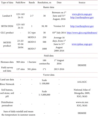
5. Data Used and Pre-Processing

5.1. Data Used

The main goal of the study was to create more accurate input maps using satel-lite imagery and ground measurement data such as soil humus, soil texture, soil permeability, agro-climate condition, and hydrothermal in land suitability eval-uation for agricultural cropland. In order to implement this three different data-sets were used; satellite data, biomass data from field surveys, and field survey

soil data (Table 1). In the subsequent analysis Random forest (RF) and Partial

least square (PLS) regressions were used.

5.2. Data Pre-Processing

DOI: 10.4236/gep.2017.59017 245 Journal of Geoscience and Environment Protection Table 1. Used data.

Type of data Path/Row Bands Resolution, m Date Source Raster data

Landsat 8 123-143/ _24-31 2-7 30 Between on 1 st

June and 31st August, 2016

www.glovis.usgs.gov http://earthexplorer.gov

SRTM DEM 123-143/ _24-31 1 30, 90 Version 5.0 http://earthexplorer.gov

GLC product - LC type 30 03rd _{July 2014 http://www.glcn.org/databases/}

MODIS product

23-25/ 03-04 26/04

MOD13 250 Average 16

days, from 1st June to 31st

August 2000-2016

www.ipdaac.usgs.gov

MOD15 500

MOD17 1000

Field data

Biomass data 969 sites 1 hectare _centner/ha 100 1st August ₂₀₁₆

IRIMHE Field survey

soil data 137 sites 501 plots 1*1 2013-2016 Vector data

Land use data - - _Scale

1: 100,000

-

AALAGC

River Network - - -

Soil humus, soil stone, soil

pH - -

Scale

1: 5,000,000 -

National Atlas of Mongolia, 2009,

IGG, MAS

Distribution

permafrost - - - - www.eic.mn IGG, MAS

Sum of daily rainfall and mean

the temperature in summer season - - IRIMHE

SRTM—Shuttle radar topographic mission; DEM—digital elevation model, MODIS—moderate-resolution imaging spectroradiometer; GLC—global land cover; LC—land cover; IGG—Institute of Geography and Geoecology; MAS—Mongolian Academy of Sciences; IRIMHE—Information and Research Institute of

Meteorology, Hydrology and Environment; AALAGG—Agency of Administration of Land Affair, Geodesy

and Cartography.

pheric model, a rural aerosol model, no aerosol retrieval and 40 km initial visi-bility. These were generated from the six bands of the surfaces’ reflectance im-ages. In this study 104 scenes of Landsat 8 satellite were analyzed, and the pri-mary difficulty was the associated color balance. In order to address this we used the MOSPREP algorithm with the bundle color balancing method in PCI GEOMATICA. The bundle color balancing method applies a global adjustment of the mean and sigma of each image using a “block-bundle” method between it and each of its overlapping images, and then, using dodging points, makes smaller local adjustments between pairs of images once they have been

mo-saicked (www.pcigeomatics.com).

DOI: 10.4236/gep.2017.59017 246 Journal of Geoscience and Environment Protection

file format and coordinate system, and then apply the atmospheric correction. Using MRT (MODIS re-projection tools) we can read input datasets in HDF- EOS, which were then converted to the UTM coordinate system with a changed file format (*.tiff). The generated surfaces’ reflectance images each used atmos-pheric correction as implemented in the QGIS2.18 SCP plugin. All image pre-processing used QGIS 2.18, ArcMap 10.4, PCI, Geomatica, ENVI v5.1, and RStudio.

Data validations accuracy assessment RF and PLS were calculated to compare with field survey soil and biomass data. RF regression was chosen because RF is a statistical algorithm that is capable of synthesizing regression or classification

functions based on discrete or continuous datasets [37]. RF and CDT regression

analyses were performed in Salford predictive Modeler 8.0 software. We also used PLS regression because the main goal of PLS regression is to predict or analyze a set of dependent variables from a set of independent variables or

pre-dictors [38]. PLS can easily treat data from a large number of variables in each

factor that is identified [39]. Finally, all vector data were converted to raster

format and then, all raster format data were transformed to the same geographi-cal coordinate system and spatial resolution (30 m). Thereafter, each criterion map was classified into five suitability classes applying the classification thre-shold values of each criteria and standard scores for the corresponding class ob-tained in Table 2.

6. Analysis

The analysis comprised of three phases; the development of criteria parameters in land suitability evaluation for agricultural cropland; the preparation of more accurate input data using high-resolution satellite image, and an integrated evaluation.

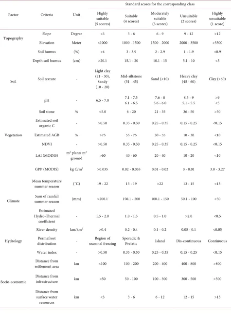
6.1. Develop Criteria Parameters for Land Suitability

Evaluation for Agricultural Cropland

6 main factors and 17 criteria for land suitability evaluation for agricultural cropland were selected. A criteria evaluation schema was then developed based on our own, and other countries practices, literature and expert knowledge (Table 2, Table 3). The criteria evaluation were divided into two types, mul-ti-variables (factor) and constraint criteria parameters.

DOI: 10.4236/gep.2017.59017 247 Journal of Geoscience and Environment Protection Table 2. Evaluation of the multi-variable (factor) criteria parameters.

Factor Criteria Unit

Standard scores for the corresponding class Highly

suitable (5 scores)

Suitable (4 scores)

Moderately suitable (3 scores)

Unsuitable (2 scores)

Highly unsuitable (1 score)

Topography Slope Degree <3 3 - 6 6 - 9 9 - 12 >12

Elevation Meter <1000 1000 - 1500 1500 - 2000 2000 - 3500 >3500

Soil

Soil humus (%) >4 3 - 3.9 2 - 2.9 1 - 1.9 <0.9

Depth soil humus (cm) >20.1 15.1 - 20 10.1 - 15 5.1 - 10 <5

Soil texture -

Light clay (21 - 30), Sandy (10 - 20)

Mid-siltstone

(31 - 45) Sand (<10) Heavy clay (45 - 60) Clay (>60)

pH - 6.5 - 7.0 7.1 - 7.5 _{6.1 - 6.5 5.6 - 6.0} 7.6 - 8 _{5.1 - 5.5} 8.5 - 9 >9 _<5

Soil stone % <5.0 6 - 20 21 - 35 36 - 50 >50

Estimated soil

organic C - >0.50 0.35 - 0.50 0.25 - 0.35 0.15 - 0.25 <0.15

Vegetation Estimated AGB % >75 55 - 75 30 - 55 10 - 30 <10

NDVI - >0.50 0.35 - 0.50 0.25 - 0.35 0.15 - 0.25 <0.15

LAI (MODIS) m2 plant/ m_ground 2 >60 40 - 60 20 - 40 10 - 20 <10

GPP (MODIS) kg C/m2 _{>0.035 0.02 - 0.035 0.01 - 0.02 0 - 0.01 3.0 - 3.27}

Climate

Mean temperature

summer season (˚C) 19 - 22 15 - 19 >22 13 - 15 <13

Sum of rainfall

summer season (mm) >200.1 150.1 - 200 100.1 - 150 50.1 - 100 <50

Estimated Hydro-Thermal

coefficient - 1.5 - 2.0 1.0 - 1.5 0.5 - 1.0 >2.0 <0.5

Hydrology

River density km/km2 _{>0.4 0.2 - 0.4 0.1 - 0.2 0.05 - 0.1 <0.05} Permafrost

distribution - seasonal freezing Region of Sporadic & Prelatic Island Dis-continuous Continuous Water index - >0.50 0.35 - 0.50 0.25 - 0.35 0.15 - 0.25 <0.15

Socio-economic

Distance from

settlement area km <100 100 - 200 200 - 400 400 - 800 >800

Distance from

infrastructure km <50 50 - 100 100 - 300 300 - 500 >500

Distance from surface water

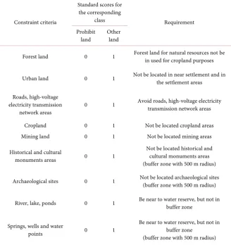
DOI: 10.4236/gep.2017.59017 248 Journal of Geoscience and Environment Protection Table 3. Evaluation of the constraint criteria parameters.

Constraint criteria

Standard scores for the corresponding

class _Requirement

Prohibit

land Other land

Forest land 0 1 Forest land for natural resources not be _{in used for cropland purposes}

Urban land 0 1 Not be located in near settlement and in _{the settlement areas}

Roads, high-voltage electricity transmission

network areas 0 1

Avoid roads, high-voltage electricity transmission network areas

Cropland 0 1 Not be located cropland areas

Mining land 0 1 Not be located mining areas

Historical and cultural

monuments areas 0 1

Not be located historical and cultural monuments areas (buffer zone with 500 m radius)

Archaeological sites 0 1 Not be located archaeological sites _{(buffer zone with 500 m radius)}

River, lake, ponds 0 1 Be near to water reserve, but not in _{buffer zone}

Springs, wells and water

points 0 1

Be near to water reserve, but not in buffer zone

(buffer zone with 500 m radius)

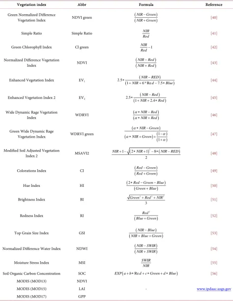
6.2. Prepare More Accurate Input Data Using High-Resolution

Satellite Image

Complex natural factors are nearly impossible to express by quantitative and qu-alitative values with 100 percent conviction. In order to improve accuracy, vari-ous analytical methods and satellite images were used. In this section we at-tempted to estimate vegetation parameters, soil organic matter, soil texture, soil moisture, and agro-climatic conditions for the hydrothermal coefficient using Landsat 8 image and MODIS products (MOD11, MOD13, MOD15, MOD17) that used the follow indices (Table 4).

6.2.1. Topography Factor Analysis

DOI: 10.4236/gep.2017.59017 249 Journal of Geoscience and Environment Protection Table 4. Vegetation & other indices used in this study.

Vegetation index Abbr Formula Reference

Green Normalized Difference

Vegetation Index NDVI green

( )

(NIRNIR GreenGreen)

−

+ [40]

Simple Ratio Simple Ratio NIR

Red [41]

Green Chlorophyll Index Cl green NIR 1

Red− [42]

Normalized Difference Vegetation

Index NDVI

( )

(NIRNIR RedRed)

−

+ [43]

Enhanced Vegetation Index EV1 2.5 ₍ ( ) ₎

1 6 * Re 7.5

NIR RED

NIR d Blue

− ∗

+ + − ∗ [44]

Enhanced Vegetation Index 2 EV2 2.5 ₍ ( ) ₎

1 2.4

NIR Red

NIR Red

− ∗

+ + ∗ [45]

Wide Dynamic Rage Vegetation

Index WDRVI

( )

( NIRNIR RedRed)

α α

∗ −

∗ + [46]

Green Wide Dynamic Rage

Vegetation Index WDRVI green

( )

( ) (₍1 )₎

1 NIR Green NIR Green α α α α ∗ − − ∗ + + + [47]

Modified Soil Adjusted Vegetation

Index 2 MSAVI2 ( ) ( )

2

1 2 1 8 2

NIR+ − ∗NIR+ − ∗ NIR−RED [48]

Colorations Index CI (₍Red Green)₎

Red Green

−

+ [49]

Hue Index HI (2∗Red_(Green−Green_+Blue−₎Blue) [50]

Brightness Index BI 2 2 2

3

Green +Red +NIR _[51]

Redness Index RI _{( )}

2

Red

Blue Green+ [52]

Top Grain Size Index GSI ₍ (NIR Blue) ₎

NIR Blue Green

−

+ + [53]

Normalized Difference Water Index NDWI (₍NIR SWIR)₎

NIR SWIR

−

+ [54]

Moisture Stress Index MSI SWIR

NIR [55]

Soil Organic Carbon Concentration SOC EXP a( + ∗b Red+ ∗c Green+ ∗d Blue) [56]

MODIS (MOD13) NDVI

- www.ipdaac.usgs.gov

MODIS (MOD15) LAI

MODIS (MOD17) GPP

DOI: 10.4236/gep.2017.59017 250 Journal of Geoscience and Environment Protection

6.2.2. Vegetation Factor Analysis

Stable natural vegetation growing areas can be represented as a habitat in areas with crop vegetation. Natural vegetation parameters can provide an additional

source of information for regional agro-production use [43]. Therefore, in this

study vegetation indices estimated from Landsat 8 satellite image were compared with the 969 sites’ biomass data from the field survey. By comprehensively ana-lyzing 553 sites of the biomass data, 416 sites’ data were eliminated because 31 sites had no data, 21 were too biased, and another 365 sites’ data depended on the temporal resolution of the Landsat 8 image.

1) Partial Least Squares (PLS) regression result

A total of 17 indices were selected to analyze the correlation between measured AGB and Landsat 8 images. There were 14 vegetation indices, 2 moisture indices and 1 soil index. PLS regression analysis was performed with SPSS software.

The strongest correlation between AGB and Landsat indices were detected in the Cl green (0.89), simple ratio (0.89), WDRVI (0.87), NDVI (0.84), EV1 (0.84), EV2 (0.80), and MSAVI2 (0.80) as a result of the PLS regression. Correlation between AGB and Landsat 8 indices showed 11 linear indices and 6 nonlinear indices. The general correlation between AGB and Landsat indices were defined

by the result of the PLS regression at R2 _{0.749, RMSE 1.011. In other words, AGB}

from Landsat 8 satellite image was estimated at 75% confidence and a linear regression was obtained.

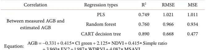
In the four abovementioned analyses, we obtained the 6 most important

vari-ables to evaluate AGB, the Cl green, simple ratio, NDVI, EV2, WDRVI and

MSAVI2. We then calculated six vegetation indices using Landsat 8 to estimate

AGB across the study area. The results are shown in Table 5.

We explored the relationship between estimated AGB and MODIS time-series vegetation products (NDVI, LAI, GPP), to understand the major controls of es-timated AGB. Our country on average, has a 5-month natural growing season (April to August). At about the end of April and the start of May the grass turns green. June is the primary period of grass growth. The growth slows down to-ward the end of August, then the grass begins to fade. Therefore, in this study the MODIS vegetation products (NDVI, LAI, and GPP) covering the period from the beginning of June to the end of August was used, ranging from the year 2000 to 2016. The performed regression analyses were used to evaluate the rela-tionship between estimated AGB and the 17-year average MODIS vegetation products.

Table 5. The result of regression models.

Correlation Regression types R2 _{RMSE MSE}

Between measured AGB and estimated AGB

PLS 0.749 1.021 1.011

Random forest 0.760 0.966 0.934 CART decision tree 0.890 0.668 0.477

DOI: 10.4236/gep.2017.59017 251 Journal of Geoscience and Environment Protection

6.2.3. Soil Factor Analysis

Parameters of soil properties mirror the land suitability evaluation for agricul-tural cropland. The spectral response of soil is influenced by a number of soil re-lated properties such as surface condition, particle size (texture), organic matter,

soil color, moisture content, iron and iron oxide content and mineralogy [57]. It

is also possible to obtain soil property estimations from remotely sensed images

[58]. Several studies attempted to demonstrate the relationship between soil

properties and reflectance data from satellite imagery [56][58] [59] [60] [61]

[62]. From these studies, a logarithmic linear relationship for organic C was

de-veloped by Chen et al. This linear equation utilizes image intensity in Red, Green and Blue bands and it is widely used to evaluate soil organic properties [58][60]. In this study, Chen’s equation was used for the evaluation of the soil’s organic carbon.

(

)

exp

SOC= a+ ∗ + ∗ + ∗b R c G d B (6)

SOC is the surface organic C; a, b, c and d are curve fit parameters

(a=1.71499, b= −0.01576, c=0.01281, d = −0.0113); R, G and B are

wa-velength ranges.

6.2.4. Agro-Climatic Factor Analysis

Agro-climatic factors establish a quantitative connection between vegetative

processes of specific plants and their in situ atmospheric environment [63].

Mongolia has an extreme continental climate with great variation between the four seasons. It has long, cold winters and short summers, with more than 65% of its annual precipitation falling in the summer season. In the summer season, the precipitation amount and daily mean air temperature affect plant growth rate. Data from 55 meteorological stations between 1940 and 2013 show that annual precipitation averages 153 mm in the summer season (from June to

Au-gust), and the mean air temperature is 17.5˚C (http://www.eic.mn/climate/). In

Mongolia, the temperature threshold that allows growth and biomass produc-tion to begin is generally +5˚C. The time period with daily temperature means at or above this threshold is approximately 150 - 165 days. One of the most impor-tant parameters to evaluate agro-climatic conditions is the hydrothermal coeffi-cient (HTK). HTK is the sum of precipitation compared with the sum of the daily temperature in the vegetation period. In this research HTK has been esti-mated based on Selyaninov’s formula.

C 0.1

i i

X P HTK

T>

=

 ∗ 

 

∑

∑

(7)

i

HTK —HydroThermal coefficient.

P

∑

C

X T_>

∑

X

DOI: 10.4236/gep.2017.59017 252 Journal of Geoscience and Environment Protection

number and duration of rain types over Mongolia from 1981 to 2014” [64]. The

maps were created in the 2010s, by the joint research efforts of the “Asia Re-search Center, National University of Mongolia (NUM)” and the Information and Research Institute of Meteorology, Hydrology and Environment (IRIMHE). This study used daily precipitation and temperature data recorded during the summer season (from June to August) between 1981 and 2014 from 55 meteo-rological stations throughout Mongolia. These maps were converted to thematic GIS layers.

7. Results

In this study a combination of constraint and factor analysis methods were used. There were nine constraint factors and 17 criteria factors. All constraints can be represented with values of 0 or 1. Suitability levels between 0 and 5 were obtained for each of the factors. The levels were 5—highly suitable, 4—suitable, 3—mode- rately suitable, 2—unsuitable and l—highly unsuitable (Table 2, Table 3).

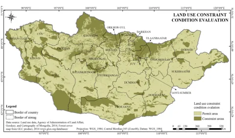
7.1. Result of Constraint Factor Analysis Based on Boolean

Logic Theory

Assessment of the land use constraint conditions was determined by the sum of factors restricting land usage. The constraint factor assessment of land use is represented by a true or false condition. A zero value means impossible, and a 1 value means possible. We defined the forest, urban area, roads, high-voltage electricity transmission network areas, mining areas, historical and cultural monument areas, archaeological sites, rivers, lakes, springs, wells and water points (near to water reserve, but not in buffer zone) as completely unsuitable for cropland based on current land-use policy in Mongolia. Using the weighted linear combination method all constraint factors were combined. The analysis

demonstrated a 31.2% constraint factor for the entirety of Mongolia (Figure 3).

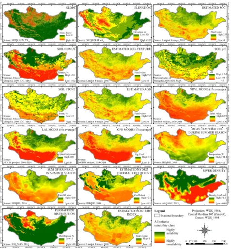
7.2. Result of Factor Analysis Based on the Spatial MCDM Method

A comprehensive analysis of the study area used six major factors (topography, soil, vegetation, agro-climate, hydrology and socio-economic) for land suitability evaluation at the primary level. There were a different number of criteria under

each category totaling 22 at the secondary level (Table 2, column 2). In this

DOI: 10.4236/gep.2017.59017 253 Journal of Geoscience and Environment Protection Figure 3. Land use constraint condition evaluation (Boolean map method).

changing dominance in different areas, the same environmental factors could have dissimilar influences.

Figure 4 shows the suitability value maps for 17 criteria, which represent the distribution of the suitability values within the study area using a continuous scale with values ranging from low to high.

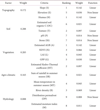
7.3. Results of Ranking and Weights Analysis of the Criteria

Based on the AHP Method

Table 6 shows the ranking of 17 factors based on a literature review and expert consultations, with the weights calculated using AHP based GIS. In this study we have estimated a CR = 0.089, suggesting that there was a reasonable level of con-sistency in judgement.

7.4. Result of Map Layer Overlay Analysis Based on

Suitability Index

After weighing the importance of different criteria for land suitability analysis, seventeen criteria maps were overlaid using the suitability index.

0.142 S 0.030 * E 0.142 H 0.021 OC 0.097 T 0.014 P 0.014 SS 0.0142 A 0.066N 0.045 L 0.030 G 0.097 HT 0.021 SR 0.045MT 0.069 R 0.008 DP 0.011 M

i

S ∗ + + ∗ + ∗ + ∗ + ∗

+ ∗ + ∗ + + ∗ + ∗ + ∗

+ ∗ + + ∗ + ∗ + ∗

=

DOI: 10.4236/gep.2017.59017 254 Journal of Geoscience and Environment Protection Figure 4. The main factors used in cropland suitability evaluation.

The results of the integrated assessment of constraint and factor analysis are

shown in Figure 6, and Table 7. The integrated assessment shows that 10.1% of

the area covered was highly suitable, 14.0% suitable, 15.5% moderately suitable,

16.3% unsuitable, 12.9% highly unsuitable and 31.2% was the constraint area.

7.5. Accuracy Assessment

DOI: 10.4236/gep.2017.59017 255 Journal of Geoscience and Environment Protection Table 6. Defined ranking and weights of the criteria.

Factor Weight Criteria Ranking Weight Function

Topography 0.172 Slope (S) 1 0.142 Linear

Elevation (E) 5 0.030 Non linear

Soil 0.288

Humus (H) 1 0.142 Linear

Estimated soil

organic C (OC) 6 0.021 Linear

Texture (T) 2 0.097 Linear

pH (P) 7 0.014 Non linear

Stone (SS) 7 0.014 Non linear

Vegetation 0.283

Estimated AGB (A) 1 0.142 Linear

NDVI (N) 3 0.066 Linear

LAI (L) 4 0.045 Linear

GPP (G) 5 0.030 Linear

Agro-climatic 0.163

Estimated Hydro-Thermal

coefficient (HT) 2 0.097 Linear

Sum of rainfall in summer

season (SR) 6 0.021 Linear

Mean temperature in

summer season (MT) 4 0.045 Linear

Hydrology 0.088

River density (R) 3 0.069 Linear Distribution permafrost

(DP) 9 0.008 Non linear

Estimated moisture index

(M) 8 0.011 Linear

Consistency ratio (CR): 0.089.

Table 7. Suitability classification results for cropland in Mongolia.

Suitability classification

Preliminary study result

(used thematic map) Current study result(used satellite data) Area, km2 _{% of total area Area, km}2 _{% of total area}

Highly suitable 83,030 5.30 157,707.5 10.1

Suitable 222,457 14.2 219,716.4 14.0

Moderately suitable 452,747 28.9 243,498.4 15.5

Unsuitable 249,089 15.9 255,180.5 16.3

Highly unsuitable 65,797 4.20 201,514.7 12.9

Constraint area* 482,513 30.8 488,982.5 31.2

Constraint area* is unsuitable based on current land-use policy.

(PLS) regression. The general accuracy is 88%, while PLS and RF regression are

82.3% and 92.8%, respectively (Graphic 1, Graphic 2). The results were then

DOI: 10.4236/gep.2017.59017 256 Journal of Geoscience and Environment Protection Figure 5. Suitable sites for cropland development (Multi-criteria factor analysis).

Figure 6. Suitability classification map for cropland in Mongolia.

Figure 7 and Table 8.

8. Conclusion

DOI: 10.4236/gep.2017.59017 257 Journal of Geoscience and Environment Protection Graphic 1. The relationship between AGB and suitability classification map for cropland by RF regression results.

Graphic 2. The correlation between AGB and suitability classification map for cropland and PLS regression results.

DOI: 10.4236/gep.2017.59017 258 Journal of Geoscience and Environment Protection Figure 7. Evaluation validation.

Table 8. Comparison of results with sown area.

Suitability classification Comparison of results (%)

Preliminary study result Current study result

Highly suitable 30.0 82.4

Suitable 67.5 16.2

Moderately suitable 1.80 1.40

Unsuitable 0.40 -

Highly unsuitable 0.00 -

and it allows for the possibility of justifying policy decisions with science.

Acknowledgements

The authors would like to thank a number of organizations who provided data for this study: The Information and Research Institute of Meteorology, Hydrol-ogy and Environment (IRIMHE); The Agency of Administration of Land Affairs, Geodesy & Cartography; and InjGeoTech LLC. We thank the EURASIA-PACIFIC UNINET/Ernst Mach Scholarship program for financial support. We are grate-ful to Gerhard Mocza, Markus Immitzer, Martin and Francesco Vuolo who are researchers of the Natural Resources and Life Sciences (BOKU) for their assis-tance in this research. We thank all colleagues at the Institute of Geography and Geoecology, Mongolian Academy of Sciences who helped in this study.

References

DOI: 10.4236/gep.2017.59017 259 Journal of Geoscience and Environment Protection Independent Agricultural Cropland Sector in Mongolia. Proceeding of theNational Conference ATAR-50, Ulaanbaatar, 23 November 2009,4-19.

[2] National Statistics Office of Mongolia (2016) Total Sown Area Data between 1960-2016 Years. Mongolian Statistical Information Service, Ulaanbaatar.

http://www.1212.mn

[3] National Statistic Committee (2016) Methodology of Estimate of Food Security Sta-tistical Parameters. The Technical Note of Mongolian National Statistic Committee, Ulaanbaatar, 1-25.

http://www.sukhbaatar.nso.mn/uploads/users/16/files/argachlal/cafc3khunsnii_ayul gvi_baidal.pdf

[4] Mongolian Customs (2016) Food Vegetables Import Data between 1995-2016 Years. Statistical Information System, Ulaanbaatar.

http://customs.gov.mn/statistics/

[5] Munkhdulam, O. and Jargaltulga, T. (2016) Agricultural Cropland Suitability Eval-uation in Mongolia. The Project Report Land Suitability EvalEval-uation in Mongolia. In: Mygmarjav, M., Ed., Eng-GeoTech LLC and Institute of Geography, Mongolian Academy of Sciences, Ulaanbaatar, 1-134.

[6] Clement, A. (2013) Advances in Remote Sensing of Agriculture: Context Descrip-tion, Existing Operational Monitoring Systems and Major Information Needs. Re-mote Sensing,5, 949-981. http://www.mdpi.com/2072-4292/5/2/949

https://doi.org/10.3390/rs5020949

[7] Clement, A., Jacques, D. and Anja, K. (2008) Smoothing Time Series of Satel-lite-Derived Vegetation Indices for Global Monitoring of Agricultural Productivity and Food Security. Joint Research Center (JRC) of the European Commission, IPSC, Agriculture Unit, Ispra.

[8] Eastman, J.R., Jin, W., Kyem, A.K. and Toledano, J. (1995) Raster Procedures for Multi-Criteria/Multi-Objective Decisions. Photogrammetric Engineering and Re-mote Sensing,61, 539-547.

[9] Deng, F., Li, X., Wang, H., Zhang, M. and Li, R. (2014) GIS-Based Assessment of Land Suitability for Alfalfa Cultivation: A Case Study in the Dry Continental Steppes of Northern China. Spanish Journal of Agricultural Research,12, 364-375.

https://doi.org/10.5424/sjar/2014122-4672

[10] Burrough, P.A. (1992) Development of Intelligent Geographical Information Sys-tems. International Journal of Geographical Information Systems,6, 1-11. https://doi.org/10.1080/02693799208901891

[11] Prakash, T.N. (2003) Land Suitability Analysis for Agricultural Crops: A Fuzzy Multicriteria Decision Making Approach. International Institute for Geo-Infor- mation Science and Earth Observation Enschede, 1-68.

http://www.iirs.gov.in/iirs/sites/default/files/StudentThesis/final_thesis_prakash.pdf [12] Ceballos-Silva, A. and López-Blanco, J. (2003) Delineation of Suitable Areas for

Crops using a Multi-Criteria Evaluation Approach and Land Use-Cover Mapping: A Case Study in Central Mexico. Agricultural Systems,77, 117-136.

[13] Malczewski, J. (1999) GIS and Multicriteria Decision Analysis. John Wiley and Sons, Inc.

[14] Malczewski, J. (2004) GIS-Based Land-Use Suitability Analysis: A Critical Overview. Progress in Planning,62, 3-65.

DOI: 10.4236/gep.2017.59017 260 Journal of Geoscience and Environment Protection [16] Banai, R. (1993) Fuzziness in Geographical Information Systems: Contribution from the Analytic Hierarchy Process. International Journal of Geographical Infor-mation Science,7, 315-329. https://doi.org/10.1080/02693799308901964

[17] Eastman, J.R. (1997) Idrisi for Windows, Version 2.0: Tutorial Exercises. Graduate School of Geography-Clark University, Worcester.

[18] Thill, J.C. (2000) Geographic Information Systems for Transportation in Perspec-tive. Transportation Research Part C. Emerging Technologies, 8, 1-6.

[19] Sui, D.Z. (1994) Recent Applications of Neural Networks for Spatial Data Handling. Canadian Journal of Remote Sensing,20, 368-380.

https://doi.org/10.1080/07038992.1994.10874580

[20] Chen, Y., Yu, J., Shahbaz, K. and Xevi, E. (2009) A GIS-Based Sensitivity Analysis of Multi-Criteria Weights. 18th World Images Congress and Modsim 09 International Congress on Modelling and Simulation, Cairns, 13-17 July 2009, 3137-3143.

http://mssanz.org.au/modsim09

[21] Dermirel, T., Demirel, N.C. and Kahraman, C. (2009) Fuzzy Analytic Hierarchy Process and Its Application. In: Kahraman, C., Ed., Fuzzy Multi-Criteria Decision Making: Theory and Applications with Recent Developments,16, 53-84.

[22] Zhang, K. and Achari, G. (2010) Uncertainty Propagation in Environmental Deci-sion Making using Random Sets. Procedia Environmental Sciences,2, 576-584. [23] Zarghami, M., Szidarovszky, F. and Ardakanian, R. (2008) A Fuzzy-Stochastic

OWA Model for Robust Multi-Criteria Decision Making. Fuzzy Optimization and Decision Making,7, 1-15.

https://link.springer.com/article/10.1007%2Fs10700-007-9021-y?LI=true

https://doi.org/10.1007/s10700-007-9021-y

[24] Mosadeghi, R., Warnken, J., Tomlinson, R. and Mirfenderesk, H. (2013) Uncer-tainty Analysis in the Application of Multi-Criteria Decision-Making Methods in Australian Strategic Environmental Decisions. Journal of Environmental Planning and Management,56, 1097-1124.https://doi.org/10.1080/09640568.2012.717886

[25] McBratney, A.B. and Odeh, I.A. (1997) Application of Fuzzy Sets in Soil Science: Fuzzy Logic, Fuzzy Measurements, and Fuzzy Decisions. Geoderma,77, 85-113. [26] Collins, M.G., Steiner, F.R. and Rushman, M.J. (2001) Land-Use Suitability Analysis

in the United States: Historical Development and Promising Technological Achieve-ments. Environmental Management, 25, 611-621.

https://doi.org/10.1007/s002670010247

[27] Zadeh, L.A. (1965) Fuzzy Sets. Information and Control,8, 338-353.

[28] Ligmann-Zielinska, A. (2013) Spatially-Explicit Sensitivity Analysis of an Agent-Based Model of Land Use Change. International Journal of Geographical Information Science,25, 1764-1781.https://doi.org/10.1080/13658816.2013.782613

[29] Joerin, F., Thériault, M. and Musy, A. (2001) Using GIS and Outranking Multicrite-ria Analysis for Land-Use Suitability Assessment. International Journal of Geo-graphical Information Science,15, 153-174.

https://doi.org/10.1080/13658810051030487

[30] Malczewski, J. (2006) GIS-Based Multicriteria Decision Analysis: A Survey of the Literature. International Journal of Geographical Information Science,20, 703-726. https://doi.org/10.1080/13658810600661508

DOI: 10.4236/gep.2017.59017 261 Journal of Geoscience and Environment Protection https://link.springer.com/article/10.1007%2Fs10666-006-9059-1?LI=true

https://doi.org/10.1007/s10666-006-9059-1

[32] Saaty, T.L. (1980) The Analytic Hierarchy Process. McGraw-Hill, New York. [33] Wu, F. (1998) SimLand: A Prototype to Simulate Land Conversion through the

In-tegrated GIS and CA with AHP-Derived Transition Rules. Geographical Informa-tion Science,12, 63-82.https://doi.org/10.1080/136588198242012

[34] Saaty, T.L. (2008) Decision Making with the Analytic Hierarchy Process. Interna-tional Journal of Services Sciences,1, 83-98.

https://doi.org/10.1504/IJSSCI.2008.017590

[35] Chen, Y., Yu, J. and Khan, S. (2010) Spatial Sensitivity Analysis of Multi-Criteria Weights in GIS-Based Land Suitability Evaluation. Environmental Modelling and Software,25, 1582-1591.

[36] Pascual, R., Rainer, M., David, M. and Hui, C. (2010) Spatially-Explicit Sensitivity Analysis for Conservation Management: Exploring the Influence of Decisions in Invasive Alien Plant Management. Diversity and Distributions,16, 426-438. https://doi.org/10.1111/j.1472-4642.2010.00659.x

[37] Mutanga, O., Adam, E. and Cho, M.A. (2012) High-Density Biomass Estimation for Wetland Vegetation using Worldview-2 Imagery and Random Forest Regression Algorithm. International Journal of Applied Earth Observation and Geoinforma-tion,18, 399-406.

[38] Abdi, H. (2007) Partial Least Square Regression: PLS Regression. In: Neil, S., Ed., Encyclopedia of Measurement and Statistics, 1-13.

http://www.utd.edu/~Herve/Abdi-PLSR2007-pretty.pdf

[39] Geladi, P. and Kowalski, B.R. (1986) Partial Least-Squares Regression: A Tutorial. Analytica Chimica Acta,185, 1-17.

[40] Gitelson, A.A., Kaufman, Y.J. and Merzlyak, M.N. (1996) Use of a Green Channel in Remote Sensing of Global Vegetation from EOS-MODIS. Remote Sensing of Envi-ronment,58, 289-298.

[41] Jordan, C.F. (1969) Derivation of Leaf-Area Index from Quality of Light on the Forest Floor. Ecology,50, 663-666. https://doi.org/10.2307/1936256

[42] Gitelson, A.A. (2005) Remote Estimation of Canopy Chlorophyll Content in Crops. Geophysical Research Letter,32, L08403.https://doi.org/10.1029/2005GL022688

[43] Rouse, J.W., Haas, R.H., Schell, J.A. and Deering, D.W. (1974) Monitoring Vegeta-tion Systems in the Great Plains with ERTS. NASA, Goddard Space Flight Center 3d ERTS-1 Symposium, Vol. 1, 309-317.

https://ntrs.nasa.gov/search.jsp?R=19740022614

[44] Liu, H.Q. and Huete, A.A. (1995) Feedback Based Modification of the NDVI to Mi-nimize Canopy Background and Atmospheric Noise. IEEE Transaction on Geos-cience and Remote Sensing,33, 457-465.

http://ieeexplore.ieee.org/document/370361/

https://doi.org/10.1109/36.377946

[45] Jiang, Z., Huete, A.R., Didan, K. and Miura, T. (2008) Development of a Two-Band Enhanced Vegetation Index without a Blue Band. Remote Sensing of Environment, 112, 3833-3845.

[46] Gitelson, A.A. (2004) Wide Dynamic Range Vegetation Index for Remote Quantifi-cation of Biophysical Characteristics of Vegetation. Journal of Plant Physiology, 161, 165-173.https://doi.org/10.1078/0176-1617-01176

DOI: 10.4236/gep.2017.59017 262 Journal of Geoscience and Environment Protection J.M., Hatfield, J.L. and Meyers, T. (2012) Remote Estimation of Crop Gross Primary Production with Landsat Data. Remote Sensing of Environment,121, 404-414. [48] Qi, J.A., Chehbouni, H.A.R., Kerr, Y.H. and Sorooshian, S.A. (1994) Modified Soil

Adjusted Vegetation Index. Remote Sensing of Environment,48, 119-126.

[49] Gallagher, S.J., Duddy, I.R., Quilt, P.G., Smith, A.J., Wallance, M.W., Holdgate, G.R. and Boult, P.J. (2004) The Use of Foraminiferal Colouration Index (FCI) as a Thermal Indicator and Correlation with Vitrinite Reflectance in the Sherbrook Group, Otway Basin, Victoria. Eastern Australian Basins Symposium II, Adelaide, 5, 643-653. https://www.researchgate.net/profile/Stephen_Gallagher/publication/ [50] Chen, T.-W., Chen, Y.-L. and Chien, S.-Y. (2008) Fast Image Segmentation Based

on K-Means Clustering with Histograms in HSV Color Space. 10th Workshop on Multimedia Signal Processing, Cairns, 8-10 October 2008, 322-325.

http://ieeexplore.ieee.org/abstract/document/4665097/

[51] Escadafal, R. and Bacha, S. (1996) Strategy for the Dynamic Study of Desertification. ORSTOM, 19-34. http://www.documentation.ird.fr/hor/fdi:010008392

[52] Huete, A.R. and Escadafal, R. (1991) Assessment of Biophysical Soil Properties through Spectral Decomposition Techniques. Remote Sensing of Environment,35, 149-159.

[53] Xiao, J., Shenb, Y., Gec, J., Tateishia, R., Tanga, C., Liangd, Y. and Huange, Z. (2006) Evaluating Urban Expansion and Land Use Change in Shijiazhuang, China, by using GIS and Remote Sensing. Landscape and Urban Planning,75, 69-80. [54] Gao, B.C. (1996) NDWI-A Normalized Difference Water Index for Remote Sensing

of Vegetation Liquid Water from Space. Remote Sensing of Environment, 58, 257-266.

[55] Datt, G., Ravallion, M. and World Bank (1990) Agriculture and Rural Development Department. Regional Disparities, Targeting, and Poverty in India Policy, Research, and External Affairs Working Papers. Agricultural Policies WPS, Vol. 375, 41.

http://documents.worldbank.org/curated/en/539051468750540233/pdf/multi0page. pdf

[56] Chen, F., Kissel, D.E., West, L.T. and Adkins, W. (2000) Field-Scale Mapping of Surface Soil Organic Carbon Using Remotely Sensed Imagery. Journal of Soil and Water Conservation,64, 746-753.

https://dl.sciencesocieties.org/publications/sssaj/abstracts/64/2/746

https://doi.org/10.2136/sssaj2000.642746x

[57] Dwivedi, R.S. (2001) Soil Resource Mapping: A Remote Sensing Perspective. Re-mote Sensing Reviews,20, 89-122.https://doi.org/10.1080/02757250109532430

[58] Fox, G.A. and Sabbagh, G.J. (2002) Estimation of Soil Organic Matter from Red and Near-Infrared Remotely Sensed Data Using a Soil Line Euclidean Distance Tech-nique. Soil Science Society of America Journal,66, 1922-1929.

https://doi.org/10.2136/sssaj2002.1922

[59] Seyler, F., Bernoux, M. and Cerri, C.C. (1998) Landsat TM Image Texture and Moisture Variations of the Soil Surface under the Rainforest of the Rondonia State, Brazil. International Journal of Remote Sensing,19, 1299-1317.

https://doi.org/10.1080/014311698215450

[60] Ahmed, Z. and Iqbal, J. (2014) Evaluation of Landsat TM5 Multispectral Data for Automated Mapping of Surface Soil Texture and Organic Matter in GIS. European Journal of Remote Sensing,47, 557-573.https://doi.org/10.5721/EuJRS20144731

DOI: 10.4236/gep.2017.59017 263 Journal of Geoscience and Environment Protection Coast using Landsat ETM+ and IKONOS Data. Aquatic Procedia,4, 1452-1460. [62] Slonecker, E.T., Jones, D.K. and Pellerin, B.A. (2015) The New Landsat 8 Potential

for Remote Sensing of Colored Dissolved Organic Matter (CDOM). Marine Pollu-tion Bulletin,107, 518-527.

[63] Kelgenbaeva, K. and Buchroithner, N. (2003) Modeling Soil and Climatic Condi-tions for Agricultural Suitability Assessment in the Siberian Altai. Proceedings of the 21st International Cartographic Conference (ICC) Cartographic Renaissance, Durban, 306-315.

http://icaci.org/files/documents/ICC_proceedings/ICC2003/Papers/038.pdf [64] Vandandorj, S., Munkhjargal, E., Boldgiv, B. and Gantsetseg, B. (2017) Changes in

Event Number and Duration of Rain Types over Mongolia from 1981 to 2014. En-vironmental Earth Sciences,76, 1-12.

Abbreviations

MCDM (Multi-Criteria Decision Method); AHP (Analytical Hierarchy Process); RF (Random Forest);

PLS (Partial Least Squares).

Submit or recommend next manuscript to SCIRP and we will provide best service for you:

Accepting pre-submission inquiries through Email, Facebook, LinkedIn, Twitter, etc. A wide selection of journals (inclusive of 9 subjects, more than 200 journals)

Providing 24-hour high-quality service User-friendly online submission system Fair and swift peer-review system

Efficient typesetting and proofreading procedure

Display of the result of downloads and visits, as well as the number of cited articles Maximum dissemination of your research work

Submit your manuscript at: http://papersubmission.scirp.org/