Probabilistic Graph-based Dependency Parsing
with Convolutional Neural Network
Zhisong Zhang1,2, Hai Zhao1,2,∗, Lianhui Qin1,2 1Department of Computer Science and Engineering, Shanghai Jiao Tong University, Shanghai, 200240, China
2Key Laboratory of Shanghai Education Commission for Intelligent Interaction and Cognitive Engineering, Shanghai Jiao Tong University, Shanghai, 200240, China
{zzs2011,qinlianhui}@sjtu.edu.cn,[email protected]
Abstract
This paper presents neural probabilistic parsing models which explore up to third-order graph-based parsing with maximum likelihood training criteria. Two neural network extensions are exploited for per-formance improvement. Firstly, a convo-lutional layer that absorbs the influences of all words in a sentence is used so that sentence-level information can be effec-tively captured. Secondly, a linear layer is added to integrate different order neu-ral models and trained with perceptron method. The proposed parsers are evalu-ated on English and Chinese Penn Tree-banks and obtain competitive accuracies.
1 Introduction
Neural network methods have shown great promise in the field of parsing and other related natural language processing tasks, exploiting more complex features with distributed representation and non-linear neural network (Wang et al., 2013; Wang et al., 2014; Cai and Zhao, 2016; Wang et al., 2016). In transition-based dependency pars-ing, neural models that can represent the partial or whole parsing histories have been explored (Weiss et al., 2015; Dyer et al., 2015). While for graph-based parsing, on which we focus in this work, Pei et al. (2015) also show the effectiveness of neural methods.
∗Corresponding author. This paper was partially
sup-ported by Cai Yuanpei Program (CSC No. 201304490199 and No. 201304490171), National Natural Science Founda-tion of China (No. 61170114 and No. 61272248), NaFounda-tional Basic Research Program of China (No. 2013CB329401), Major Basic Research Program of Shanghai Science and Technology Committee (No. 15JC1400103), Art and Sci-ence Interdisciplinary Funds of Shanghai Jiao Tong Univer-sity (No. 14JCRZ04), and Key Project of National Society Science Foundation of China (No. 15-ZDA041).
The graph-based parser generally consists of two components: one is the parsing algorithm for inference or searching the most likely parse tree, the other is the parameter estimation approach for the machine learning models. For the former, clas-sical dynamic programming algorithms are usu-ally adopted, while for the latter, there are vari-ous solutions. Like some previvari-ous neural methods (Socher et al., 2010; Socher et al., 2013), to tackle the structure prediction problems, Pei et al. (2015) utilize a max-margin training criterion, which does not include probabilistic explanations. Re-visiting the traditional probabilistic criteria in log-linear models, this work utilizes maximum likelihood for neural network training. Durrett and Klein (2015) adopt this method for constituency pars-ing, which scores the anchored rules with neu-ral models and formalizes the probabilities with tree-structured random fields. Motivated by this work, we utilize the probabilistic treatment for de-pendency parsing: scoring the edges or high-order sub-trees with a neural model and calculating the gradients according to probabilistic criteria. Al-though scores are computed by a neural network, the existing dynamic programming algorithms for gradient calculation remain the same as those in log-linear models.
Graph-based methods search globally through the whole space for trees and get the highest-scored one, however, the scores for the sub-trees are usually locally decided, considering only sur-rounding words within a limited-sized window. Convolutional neural network (CNN) provides a natural way to model a whole sentence. By in-troducing a distance-aware convolutional layer, sentence-level representation can be exploited for parsing. We will especially verify the effec-tiveness of such representation incorporated with window-based representation.
Graph-based parsing has a natural extension
through raising its order and higher-order parsers usually perform better. In previous work on high-order graph-parsing, the scores of high-high-order sub-trees usually include the lower-order parts in their high-order factorizations. In traditional linear models, combining scores can be implemented by including low-order features. However, for neural models, this is not that straightforward because of nonlinearity. A straightforward strategy is simply adding up all the scores, which in fact works well; another way is stacking a linear layer on the top of the representation from various already-trained neural parsing models of different orders.
This paper presents neural probabilistic mod-els for graph-based projective dependency pars-ing, and explores up to third-order models. Here are the three highlights of the proposed methods:
• Probabilistic criteria for neural network train-ing. (Section 2.2)
• Sentence-level representation learned from a convolutional layer. (Section 3.2)
• Ensemble models with a stacked linear out-put layer. (Section 3.3)
Our main contribution is exploring sub-tree scor-ing models which combine local features with a window-based neural network and global features from a distance-aware convolutional neural net-work. A free distribution of our implementation is publicly available1.
The remainder of the paper is organized as fol-lows: Section 2 explains the probabilistic model for graph-based parsing, Section 3 describes our neural network models, Section 4 presents our ex-periments and Section 5 discusses related work, we summarize this paper in Section 6.
2 Probabilistic Graph-based Dependency Parsing
2.1 Graph-based Dependency Parsing
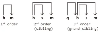
Dependency parsing aims to predict a dependency tree, in which all the edges connect head-modifier pairs. In graph-based methods, a dependency tree is factored into sub-trees, from single edge to mul-tiple edges with different patterns; we will call these specified sub-treesfactorsin this paper. Ac-cording to the sub-tree size of the factors, we can
1https://github.com/zzsfornlp/nnpgdparser
h m h s m g h s m
1st order 2nd order
[image:2.595.331.502.64.121.2](sibling) 3 rd order (grand-sibling)
Figure 1: The decompositions of factors.
define the order of the graph model. Three differ-ent ordered factorizations considered in this work and their sub-tree patterns are shown in Figure 1.
The score for a dependency tree (T) is defined as the sum of the scores of all its factors (p):
Score(T) =X
p∈T
Score(p)
In this way, the dependency parsing task is to find a max-scoring tree. For projective depen-dency parsing considered in this work, this search-ing problem is conquered by dynamic program-ming algorithms with the key assumption that the factors are scored independently. Previous work (Eisner, 1996; McDonald et al., 2005; McDonald and Pereira, 2006; Koo and Collins, 2010; Ma and Zhao, 2012) explores ingenious algorithms for de-coding ranging from first-order to higher-orders. Our proposed parsers also take these algorithms as backbones and use them for inference.
2.2 Probabilistic Model
With the graph factorization and inference, the re-maining problems are how to obtain the scores and how to train the scoring model. For the scor-ing models, traditional linear methods utilize man-ually specified features and linear scoring mod-els, while we adopt neural network modmod-els, which may exploit better feature representations.
condi-tioned on a sentenceXis defined as follows:
Pr(T|X, θ) = Z(1X)exp(Score(T|θ))
Z(X) =X
T0
exp(Score(T0|θ))
whereθrepresents the parameters andZ(X)is the re-normalization partition function. The intuition is that the higher the score is, the more potential or mass it will get, leading to higher probability.
The training criteria will be log-likelihood in the classical setting of maximum likelihood esti-mation, and we define the loss for a parse tree as negative log-likelihood:
L(θ) =−logPr(Tg|X, θ)
=−Score(Tg|θ) + log(Z(X))
where Tg stands for the golden parse tree. Now
we need to calculate the gradients ofθaccording to gradient-based optimization. Focusing on the second term, we have (some conditions are left out for simplicity):
∂log(Z(X))
∂θ =
X
T0
Pr(T0)X
p∈T0
∂Score(p)
∂θ
=X
p
∂Score(p)
∂θ
X
T0∈T(p) Pr(T0)
Here,T(p)is the set of trees that contain the fac-tor p, and the inner summation is defined as the marginal probabilitym(p):
m(p) = X
T0∈T(p) Pr(T0)
which can be viewed as the mass of all the trees containing the specified factorp. The calculation of m(p) (Paskin, 2001; Ma and Zhao, 2015) is solved by a variant of inside-outside algorithm, which is of the same complexity compared with the corresponding inference algorithms. Finally, the gradients can be represented as:
∂L(θ)
∂θ =
X
p
∂Score(p)
∂θ
−p∈Tg+m(p)
where[p ∈ Tg]is a binary value which indicates
whetherpis in treeTg.
Traditional models usually utilize linear func-tions for the Score function, which might need carefully feature engineering such as (Zhao et al., 2009a; Zhao et al., 2009b; Zhao et al., 2009c; Zhao, 2009; Zhao et al., 2013), while we adopt neural models with the probabilistic training crite-ria unchanged.
2.3 Training Criteria
We take a further look between the maximum-likelihood criteria and the max-margin criteria. For the max-margin method, the loss is the differ-ence between the scores of the golden tree and a predicted tree, and its sub-gradient can be written in a similar form:
∂Lm(θ) ∂θ =
X
p
∂Score(p)
∂θ
−p∈Tg+p∈Tb
Here, the predicted treeTb is the best-scored tree
with a structured margin loss in the score.
Comparing the derivatives, we can see that the one of probabilistic criteria can be viewed as a soft version of the max-margin criteria, and all the possible factors are considered when calcu-lating gradients for the probabilistic way, while only wrongly predicted factors have non-zero sub-gradients for max-margin training. This observa-tion is not new and Gimpel and Smith (2010) pro-vide a good review of several training criteria. It might be interesting to explore the impacts of dif-ferent training criteria on the parsing performance, and we will leave it for future research.
2.4 Labeled Parsing
In a dependency tree, each edge can be given a la-bel indicating the type of the dependency relation, this labeling procedure can be integrated directly into the parsing task, instead of a second pass af-ter obtaining the structure.
For the probabilistic model, integrating labeled parsing only needs some extensions for the in-ference procedure and marginal probability cal-culations. For the simplicity, we only consider a single label for each factor (even for high-order ones) which corresponds to Model 1 in (Ma and Hovy, 2015): the label of the edge between head and modifier word, which will only multiplyO(l)
to the complexity. We find this direct approach not only achieves labeled parsing in one pass, but also improves unlabeled attachment accuracies (see Section 4.3), which may benefit from the joint learning with the labels.
3 Neural Model
in-This is a good game . DT JJ NN
Modifier Sibling Head
Embdding Hidden2 Output
Hidden1
s = Wsh2 + bs
h2 = tanh(W2h1 + b2)
h1 = tanh(W1h0 + b1)
[image:4.595.92.270.63.204.2]h0
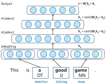
Figure 2: The architecture for the basic model (second order parsing).
tegrate features from both local word-neighboring windows and the entire sentence, and furthermore explore ensemble models with different orders.
3.1 Basic Local Model
Architecture The basic model uses a window-based approach, which includes only surround-ing words for the contexts. Figure 2 illustrates a second-order sibling model and models of other orders adopt similar structures. It is simply a stan-dard feed-forward neural network with two hid-den layers (h1andh2) above the embedding layer
(h0), the hidden layers all adopt tanh activation
function, and the output layer (noted ass) directly represents the scores for different labels.
Feature Sets All the features representing the input factor are atomic and projected to embed-dings, then the embedding layer is formed by con-catenating them. There are three categories of fea-tures: word forms, POS (part-of-speech) tags and distances. For each node in the factor, word forms and POS tags of the surrounding words in a spec-ified window are also considered. Special tokens for start or end of sentences, root node and un-known words are added for both word forms and POS tags. Distances can be negative or positive to represent the relative positions between the factor nodes in surface string. Take the situation for the second-order model as an example, there are three nodes in a factor: hfor head,mfor modifier and
sfor sibling. When considering three-word win-dows, there will be three word forms and three tags for each node and its surrounding context. mand
sboth have one distance feature whilehdoes not have one as its parent does not exist in the factor.
Training As stated in Section 2.2, we use the maximum likelihood criteria. Moreover, we add two L2-regularizations: one is for all the weights
θ0 (biases and embeddings not included) to avoid over-fitting and another is for preventing the final output scores from growing too large. The for-mer is common practice for neural network, while the latter is to set soft limits for the norms of the scores. Although the second term is not usually adopted, it directly puts soft constraints on the scores and improves the accuracies (about 0.1% for UAS/LAS overall) according to our primary experiments. So the final loss function will be:
L0(θ) =X
p
Score(p)· −p∈Tg+m(p)
+λs·Score(p)2
+λm· kθ0k2
where λm andλs respectively represent
regular-ization parameters for model and scores. The training process utilizes a mini-batched stochastic gradient descent method with momentum.
Comparisons Our basic model resembles the one of Pei et al. (2015), but with some ma-jor differences: probabilistic training criteria are adopted, the structures of the proposed networks are different and direction information is encoded in distance features. Moreover, they simply av-erage embeddings in specified regions for phrase-embedding, while we will include sentence-embedding in convolutional model as follows.
3.2 Convolutional Model
To encode sentence-level information and obtain sentence embeddings, a convolutional layer of the whole sentence followed by a max-pooling layer is adopted. However, we intend to score a factor in a sentence and the position of the nodes should also be encoded. The scheme is to use the distance embedding for the whole convolution window as the position feature.
This is a good game . DT VBZ DT
Modifier Sibling Head Output
Lexical distance
v’ l = Wlvl + bl
vl
v’ d = Wdvd + bd
vd
[image:5.595.110.256.62.182.2]dh=-3 dm=-1 ds=-2
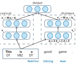
Figure 3: The operations for one convolution win-dow (second order parsing).
convolution window of “This is a”, word forms and corresponding POS tags are projected to em-beddings and concatenated as the lexical vectorvl,
the distances of the center word “is” to all the three nodes in the factor are also projected to embed-dings and concatenated as the distance vectorvd,
then these two vectors go through difference linear transformations into the same dimension and are combined together through element-wise addition or multiplication.
In general, assuming after the projection layer, embeddings of the word forms and POS tags of the sentence are represented as[w0,w1, ...,wn−1]
and[p0,p1, ...,pn−1]. Those embeddings in the
basic model may be reused here by sharing the em-bedding look-up table. The second-order sibling factor to be scored has nodes with indexes of m
(modifier),h (head) ands(sibling). The distance embeddings are denoted byd, which can be either negative or positive. These distance embeddings are different from the ones in the basic model, be-cause here we measure the distances between the convolution window (its center word) and factor nodes, while the distances between nodes inside the factors are measured in the basic model.
For a specified window[i:j], always assuming an odd number sized window, and the center token is indexed toc = i+2j, thevl andvdare obtained
through simple concatenation:
vl= [wi,pi,wi+1,pi+1, ...,wj,pj]
vd= [dc−h,dc−m,dc−s]
thenvlandvdgo through difference linear
trans-formations into same dimension space: v0l,v0d∈
Rn, where n is also the dimension of the output
vectorvo for the window. The linear operations
can be expressed as:
v0l=Wl·vl+bl
v0d=Wd·vd+bd
The final vector vo is obtained by element-wise
operations ofv0
landv0d. We consider two
strate-gies: (1) add: simple element-wise addition, (2)
mul: element-wise multiplication with v0d acti-vated bytanh. They can be formalized as:
vo-add=v0l⊕v0d
vo-mul =v0ltanh(v0d)
All the windows whose center-located word is valid (exists) in the sentence are considered and we will get a sequence of convolution outputs whose number is the same as the sentence length. The convolution outputs (allvo) are collapsed into
one global vectorvgusing a standard max-pooling
operation. Finally, for utilizing the sentence-level representation in the basic model, we can either replace the original first hidden layerh1 withvg
or concatenate vg toh1 for combining local and
global features.
3.3 Ensemble Models
For higher-order dependency parsing, it is a stan-dard practice to include the impact of lower-order parts in the scoring of higher-order factors, which actually is an ensemble method of different order models for scoring.
A simple adding scheme is often used. For non-linear neural models, we use an explicit adding method. For example, in third-order parsing, the final score for the factor(g, h, m, s)will be:
sadd(g, h, m, s) =so3(g, h, m, s) +so2(h, m, s)
+so1(h, m)
Here, g, h, m and s represent the grandparent, head, modifier and sibling nodes in the grand-sibling third-order factor;so1,so2andso3stand for
the corresponding lower-order scores from first, second and third order models, respectively.
be viewed as adopting a final layer with specially fixed weights.
For each model to be combined, we concatenate the output layer and all hidden layers (except em-bedding layerh0):
vall = [s,h1,h2]
Allvall from different models are again
concate-nated to form the input for the final linear layer and the final scores are obtained through a linear transformation (no bias adding):
vcombine= [vall-o1,vall-o2,vall-o3]
scombine=Wcombine·vcombine
We no longer update weights for the underlying neural models, and the learning of the final layer is equally training a linear model, for which struc-tured average perceptron (Collins, 2002; Collins and Roark, 2004) is adopted for simplicity.
This ensemble scheme can be extended in sev-eral ways which might be explored in future work: (1) feed-forward network can be stacked rather than a single linear layer, (2) traditional sparse fea-tures can also be concatenated tovcombineto
com-bine manually specified representations with dis-tributed neural representations as in (Zhang and Zhang, 2015).
4 Experiments
The proposed parsers are evaluated on English Penn Treebank (PTB) and Chinese Penn Tree-bank (CTB). Unlabeled attachment scores (UAS), labeled attachment scores (LAS) and unlabeled complete matches (CM) are the metrics. Punctu-ations2 are ignored as in previous work (Koo and
Collins, 2010; Zhang and Clark, 2008).
For English, we follow the splitting conven-tion for PTB3: sections 2-21 for training, 22 for developing and 23 for test. We prepare three datasets of PTB, using different conversion tools: (1) Penn2Malt3and the head rules of Yamada and
Matsumoto (2003), noted as PTB-Y&M; (2) de-pendency converter in Stanford parser v3.3.0 with Stanford Basic Dependencies (De Marneffe et al., 2006), noted as PTB-SD; (3) LTH Constituent-to-Dependency Conversion Tool4 (Johansson and 2Tokens whose gold POS tags are one of{“ ” : , .}for
PTB orP Ufor CTB.
3http://stp.lingfil.uu.se/˜nivre/research/Penn2Malt.html 4http://nlp.cs.lth.se/software/treebank converter
Nugues, 2007), noted asPTB-LTH. We use Stan-ford POS tagger (Toutanova et al., 2003) to get predicted POS tags for development and test sets, and the accuracies for their tags are 97.2% and 97.4%, respectively.
For Chinese, we adopt the splitting convention for CTB5 described in (Zhang and Clark, 2008). The dependencies (noted asCTB), are converted with the Penn2Malt converter. Gold segmentation and POS tags are used as in previous work.
4.1 Settings
Settings of our models will be described in this sub-section, including pre-processing and initial-izations, hyper-parameters, and training details.
We ignore the words that occur less than 3 times in the training treebank and use a special token to replace them. For English parsing, we initial-ize word embeddings with word vectors trained on Wikipedia usingword2vec(Mikolov et al., 2013); all other weights and biases are initialized ran-domly with uniform distribution.
For the structures of neural models, all the em-beddings (word, POS and distances) have dimen-sions of 50. For basic local models,h1andh2are
set to 200 and 100, and the local window size is set to 7. For convolutional models, a three-word-sized window for convolution is specified, and convolu-tion output dimension (number of filters) is 100. When concatenating the convolution vector (after pooling) toh1, it will make the first hidden layer’s
dimension 300.
For the training of neural network, we set the initial learning rate to 0.1 and the momentum to 0.6. After each iteration, the parser is tested on the development set and if the accuracy decreases, the learning rate will be halved. The learning rate will also be halved if no decreases of the accuracy for three epochs. We train the neural models for 12 epochs and select the one that performs best on the development set. The regularization parame-tersλmandλsare set to 0.0001 and 0.001. For the
perceptron training of the ensemble model, only one epoch is enough based on the results of the development set.
Method UAS LAS CM Basic (first-order)
Unlabeled 91.53 – 42.82
Labeled 92.13 89.60 45.06
Labeled+pre-training 92.19 89.73 45.18 Convolutional (first-order)
replace-add 92.26 89.83 44.76 replace-mul 92.02 89.61 44.24 concatenate-add 92.63 90.20 46.18 concatenate-mul 92.33 89.83 44.94 Higher-orders
o2-nope 92.85 90.51 49.65
o2-adding 93.47 91.13 51.41 o2-perceptron 93.63 91.39 51.53
o3-nope 92.47 90.01 49.06
[image:7.595.81.283.61.236.2]o3-adding 93.70 91.37 53.53 o3-perceptron 93.51 91.20 51.76
Table 1: Effects of the components, on PTB-SD
development set.
convolution model approximately takes up 40% of all computations. The convolution operation indeed costs more, but the lexical parts v0
l of
the convolution do not concern the factors and are computed only once for one sentence, which makes it less computationally expensive.
4.2 Pruning
For high-order parsing, the computation cost rises in proportion to the length of the sentence, and it will be too expensive to calculate scores for all the factors. Fortunately, many edges are quite un-likely to be valid and can be pruned away using low-order models. We follow the method of Koo and Collins (2010) and directly use the first-order probabilistic neural parser for pruning. We com-pute the marginal probability m(h, m) for each edge and prune away the edges whose marginal probability is below×maxh0m(h0, m).means
the pruning threshold that is set to 0.0001 for second-order. For third-order parsing, considering the computational cost, we set it to 0.001.
4.3 Model Analysis
This section presents experiments to verify the ef-fectiveness of the proposed methods and only the
PTB-SDdevelopment set will be used in these
ex-periments, which fall into three groups concerning basic models, convolutional models and ensemble ones, as shown in Table 1.
The first group focuses on the basic local mod-els of first order. The first two, Unlabeled and
Labeled, do not use pre-training vectors for
ini-tialization, while the third,Labeled+pre-training, utilizes them. TheUnlabeled does not utilize the
0.65 0.7 0.75 0.8 0.85 0.9 0.95 1
5 10 15 20 25 30
F1
Dependency Length labeled+pre-training (no CNN)
[image:7.595.307.530.63.200.2]replace-add (only CNN) concatenate-add (plus CNN)
Figure 4: F1 measure of different dependency lengths, onPTB-SDdevelopment set.
labels in training set and its model only gives one dependency score (we do not train a second stage labeling model, so the LAS of the unlabeled one is not available) and theLabeleddirectly pre-dicts the scores for all labels. We can see that labeled parsing not only demonstrates the conve-nience of outputting dependency relations and la-bels for once, but also obtains better parsing per-formances. Also, we observe that pre-trained word vectors bring slight improvements. Pre-trained initialization and labeled parsing will be adopted for the next two groups and the rest experiments.
Next, we explore the effectiveness of the CNN enhancement. In the four entries of this group,
concatenateorreplacemeans whether to
concate-nate the sentence-level vector vg to the first
hid-den layer h1 or just replace it (just throw away
the representation from basic models),addormul
means to use which way for attaching distance in-formation. Surprisingly, simple adding method surpasses the more complex multiplication-with-activation method, which might indicate that the direct activation operation may not be suitable for encoding distance information. With no surprises, the concatenating method works better because it combines both the local window-based and global sentence-level information. We also explore the influences of the convolution operations on depen-dencies of different lengths, as shown in Figure 4, the convolutional methods help the decisions of long-range dependencies generally. For the high-order parsing in the rest of this paper, we will all adopt theconcatenate-addsetting.
PTB-Y&M PTB-SD PTB-LTH CTB
Methods UAS LAS CM UAS LAS CM UAS LAS CM UAS LAS CM
Graph-NN:proposed
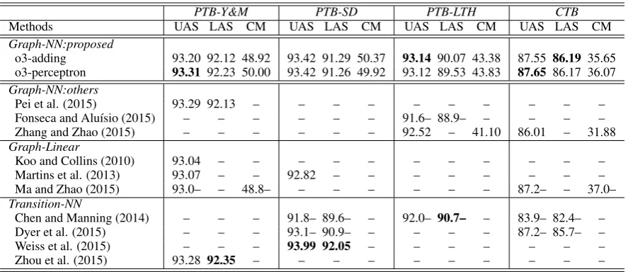
o3-adding 93.20 92.12 48.92 93.42 91.29 50.37 93.14 90.07 43.38 87.55 86.19 35.65 o3-perceptron 93.31 92.23 50.00 93.42 91.26 49.92 93.12 89.53 43.83 87.65 86.17 36.07 Graph-NN:others
Pei et al. (2015) 93.29 92.13 – – – – – – – – – –
Fonseca and Alu´ısio (2015) – – – – – – 91.6– 88.9– – – – –
Zhang and Zhao (2015) – – – – – – 92.52 – 41.10 86.01 – 31.88
Graph-Linear
Koo and Collins (2010) 93.04 – – – – – – – – – – –
Martins et al. (2013) 93.07 – – 92.82 – – – – – – – –
Ma and Zhao (2015) 93.0– – 48.8– – – – – – – 87.2– – 37.0–
Transition-NN
Chen and Manning (2014) – – – 91.8– 89.6– – 92.0– 90.7– – 83.9– 82.4– –
Dyer et al. (2015) – – – 93.1– 90.9– – – – – 87.2– 85.7– –
Weiss et al. (2015) – – – 93.99 92.05 – – – – – – –
[image:8.595.78.522.61.253.2]Zhou et al. (2015) 93.28 92.35 – – – – – – – – – –
Table 2: Comparisons of results on the test sets.
and stacking another linear perceptron layer (with the suffixes of-nope,-addingand-perceptron re-spectively). The results show that model ensemble improves the accuracies quite a few. For third-order parsing, the no-combination method per-forms quite poorly compared to the others, which may be caused by the relative strict setting of the pruning threshold. Nevertheless, with model en-semble, the third-order models perform better than the second-order ones. Though the perceptron strategy does not work well for third-order pars-ing in this dataset, it is still more general than the simple adding method, since the latter can be seen as a special parameter setting of the former.
4.4 Results
We show the results of two of the best proposed parsers: third-order adding (o3-adding) and third-order perceptron (o3-perceptron) methods, and compare with the reported results of some previ-ous work in Table 2. We compare with three cat-egories of models: other Graph-based NN (neu-ral network) models, traditionalGraph-based Lin-earmodels andTransition-basedNN models. For PTB, there have been several different dependency converters which lead to different sets of depen-dencies and we choose three of the most popular ones for more comprehensive comparisons. Since not all work report results on all of these depen-dencies, some of the entries might be not available. From the comparison, we see that the pro-posed parser has output competitive performance for different dependency conversion conventions and treebanks. Compared with traditional
graph-based linear models, neural models may benefit from better feature representations and more gen-eral non-linear transformations.
The results and comparisons in Table 2 demon-strate the proposed models can obtain comparable accuracies, which show the effectiveness of com-bining local and global features through window-based and convolutional neural networks.
5 Related Work
CNN has been explored in recent work of rela-tion classificarela-tion (Zeng et al., 2014; Chen et al., 2015), which resembles the task of deciding de-pendency relations in parsing. However, relation classification usually involves labeling for given arguments and seldom needs to consider the global structure. Parsing is more complex for it needs to predict structures and the use of CNN should be incorporated with the searching algorithms.
(Le and Zuidema, 2014) and Recursive CNN (Zhu et al., 2015), are utilized for capturing features with more contexts. However, re-ranking mod-els depend on the underlying base parsers, which might already miss the correct trees. Generally, the re-ranking techniques play a role of additional enhancement for basic parsing models, and there-fore they are not included in our comparisons.
The conditional log-likelihood probabilistic cri-terion utilized in this work is actually a (condi-tioned) Markov Random Field for tree structures, and it has been applied to parsing since long time ago. Johnson et al. (1999) utilize the Markov Ran-dom Fields for stochastic grammars and gradient based methods are adopted for parameter estima-tions, and Geman and Johnson (2002) extend this with dynamic programming algorithms for infer-ence and marginal-probability calculation. Collins (2000) uses the same probabilistic treatment for re-ranking and the denominator only includes the candidate trees which can be seen as an approx-imation for the whole space of trees. Finkel et al. (2008) utilize it for feature-based parsing. The probabilistic training criterion for linear graph-based dependency models have been also explored in (Li et al., 2014; Ma and Zhao, 2015). How-ever, these previous methods usually exploit log-linear models utilizing sparse features for input representations and linear models for score calcu-lations, which are replaced by more sophisticated distributed representations and neural models, as shown in this work.
6 Conclusions
This work presents neural probabilistic graph-based models for dependency parsing, together with a convolutional part which could capture the sentence-level information. With distributed vec-tors for representations and complex non-linear neural network for calculations, the model can ef-fectively capture more complex features when de-ciding the scores for sub-tree factors and exper-iments on standard treebanks show that the pro-posed techniques improve parsing accuracies.
References
Deng Cai and Hai Zhao. 2016. Neural word segmen-tation learning for Chinese. InProceedings of ACL, Berlin, Germany, August.
Danqi Chen and Christopher Manning. 2014. A fast and accurate dependency parser using neural
net-works. InProceedings of EMNLP, pages 740–750, Doha, Qatar, October.
Yubo Chen, Liheng Xu, Kang Liu, Daojian Zeng, and Jun Zhao. 2015. Event extraction via dynamic multi-pooling convolutional neural networks. In
Proceedings of ACL, pages 167–176, Beijing, China, July.
Michael Collins and Brian Roark. 2004. Incremen-tal parsing with the perceptron algorithm. In Pro-ceedings of the 42nd Meeting of the Association for Computational Linguistics (ACL’04), Main Volume, pages 111–118, Barcelona, Spain, July.
Michael Collins. 2000. Discriminative reranking for natural language parsing. In Proceedings of the Seventeenth International Conference on Machine Learning, pages 25–70.
Michael Collins. 2002. Discriminative training meth-ods for hidden markov models: Theory and exper-iments with perceptron algorithms. InProceedings of the ACL-02 conference on Empirical methods in natural language processing-Volume 10, pages 1–8.
Marie-Catherine De Marneffe, Bill MacCartney, Christopher D Manning, et al. 2006. Generat-ing typed dependency parses from phrase structure parses. InProceedings of LREC, volume 6, pages 449–454.
Greg Durrett and Dan Klein. 2015. Neural crf pars-ing. In Proceedings of ACL, pages 302–312, Bei-jing, China, July.
Chris Dyer, Miguel Ballesteros, Wang Ling, Austin Matthews, and Noah A. Smith. 2015. Transition-based dependency parsing with stack long short-term memory. In Proceedings of ACL, pages 334– 343, Beijing, China, July.
Jason M. Eisner. 1996. Three new probabilistic mod-els for dependency parsing: An exploration. In Pro-ceedings of the 16th International Conference on Computational Linguistics, pages 340–345, Copen-hagen, August.
Jenny Rose Finkel, Alex Kleeman, and Christopher D. Manning. 2008. Efficient, feature-based, condi-tional random field parsing. InProceedings of ACL, pages 959–967, Columbus, Ohio, June.
Erick Fonseca and Sandra Alu´ısio. 2015. A deep architecture for non-projective dependency parsing. InProceedings of the 1st Workshop on Vector Space Modeling for Natural Language Processing, pages 56–61, Denver, Colorado, June.
Kevin Gimpel and Noah A. Smith. 2010. Softmax-margin crfs: Training log-linear models with cost functions. In Proceedings of NAACL, pages 733– 736, Los Angeles, California, June.
Richard Johansson and Pierre Nugues. 2007. Ex-tended constituent-to-dependency conversion for en-glish. In16th Nordic Conference of Computational Linguistics, pages 105–112. University of Tartu. Mark Johnson, Stuart Geman, Stephen Canon, Zhiyi
Chi, and Stefan Riezler. 1999. Estimators for stochastic ”unification-based” grammars. In Pro-ceedings of the 37th Annual Meeting of the Associa-tion for ComputaAssocia-tional Linguistics, pages 535–541, College Park, Maryland, USA, June.
Terry Koo and Michael Collins. 2010. Efficient third-order dependency parsers. InProceedings of ACL, pages 1–11, Uppsala, Sweden, July.
John Lafferty, Andrew McCallum, and Fernando CN Pereira. 2001. Conditional random fields: Prob-abilistic models for segmenting and labeling se-quence data.
Phong Le and Willem Zuidema. 2014. The inside-outside recursive neural network model for depen-dency parsing. In Proceedings of EMNLP, pages 729–739, Doha, Qatar, October.
Tao Lei, Yu Xin, Yuan Zhang, Regina Barzilay, and Tommi Jaakkola. 2014. Low-rank tensors for scor-ing dependency structures. InProceedings of ACL, pages 1381–1391, Baltimore, Maryland, June. Zhenghua Li, Min Zhang, and Wenliang Chen.
2014. Ambiguity-aware ensemble training for semi-supervised dependency parsing. In Proceedings of ACL, pages 457–467, Baltimore, Maryland, June. Xuezhe Ma and Eduard Hovy. 2015. Efficient
inner-to-outer greedy algorithm for higher-order labeled dependency parsing. In Proceedings of EMNLP, pages 1322–1328, Lisbon, Portugal, September. Xuezhe Ma and Hai Zhao. 2012. Fourth-order
depen-dency parsing. In Proceedings of COLING, pages 785–796, Mumbai, India, December.
Xuezhe Ma and Hai Zhao. 2015. Probabilistic models for high-order projective dependency parsing. arXiv preprint arXiv:1502.04174.
Andre Martins, Miguel Almeida, and Noah A. Smith. 2013. Turning on the turbo: Fast third-order non-projective turbo parsers. In Proceedings of ACL, pages 617–622, Sofia, Bulgaria, August.
Ryan McDonald and Fernando Pereira. 2006. Online learning of approximate dependency parsing algo-rithms. InProceedings of EACL, pages 81–88. Ryan McDonald, Koby Crammer, and Fernando
Pereira. 2005. Online large-margin training of de-pendency parsers. InProceedings of ACL, pages 91– 98, Ann Arbor, Michigan, June.
Tomas Mikolov, Ilya Sutskever, Kai Chen, Greg S Cor-rado, and Jeff Dean. 2013. Distributed representa-tions of words and phrases and their compositional-ity. InAdvances in neural information processing systems, pages 3111–3119.
Joakim Nivre and Ryan McDonald. 2008. Integrat-ing graph-based and transition-based dependency parsers. In Proceedings of ACL, pages 950–958, Columbus, Ohio, June.
Mark A Paskin. 2001. Cubic-time parsing and learning algorithms for grammatical bigram models. Techni-cal report.
Wenzhe Pei, Tao Ge, and Baobao Chang. 2015. An effective neural network model for graph-based de-pendency parsing. In Proceedings of ACL, pages 313–322, Beijing, China, July.
Richard Socher, Christopher D. Manning, and An-drew Y. Ng. 2010. Learning continuous phrase representations and syntactic parsing with recursive neural networks. InProceedings of the NIPS-2010 Deep Learning and Unsupervised Feature Learning Workshop.
Richard Socher, John Bauer, Christopher D. Manning, and Ng Andrew Y. 2013. Parsing with compo-sitional vector grammars. InProceedings of ACL, pages 455–465, Sofia, Bulgaria, August.
Andr´e Filipe Torres Martins, Dipanjan Das, Noah A. Smith, and Eric P. Xing. 2008. Stacking depen-dency parsers. In Proceedings of ENNLP, pages 157–166, Honolulu, Hawaii, October.
Kristina Toutanova, Dan Klein, Christopher D Man-ning, and Yoram Singer. 2003. Feature-rich part-of-speech tagging with a cyclic dependency network. InProceedings of the 2003 Conference of the North American Chapter of the Association for Computa-tional Linguistics on Human Language Technology-Volume 1, pages 173–180.
Rui Wang, Masao Utiyama, Isao Goto, Eiichro Sumita, Hai Zhao, and Bao-Liang Lu. 2013. Convert-ing continuous-space language models into n-gram language models for statistical machine translation. InProceedings of EMNLP, pages 845–850, Seattle, Washington, USA, October.
Rui Wang, Hai Zhao, Bao-Liang Lu, Masao Utiyama, and Eiichiro Sumita. 2014. Neural network based bilingual language model growing for statistical ma-chine translation. InProceedings of EMNLP, pages 189–195, Doha, Qatar, October.
Peilu Wang, Yao Qian, Frank Soong, Lei He, and Hai Zhao. 2016. Learning distributed word representa-tions for bidirectional lstm recurrent neural network. InProceedings of NAACL, June.
Hiroyasu Yamada and Yuji Matsumoto. 2003. Statis-tical dependency analysis with support vector ma-chines. InProceedings of IWPT, volume 3, pages 195–206.
Daojian Zeng, Kang Liu, Siwei Lai, Guangyou Zhou, and Jun Zhao. 2014. Relation classification via con-volutional deep neural network. In Proceedings of COLING, pages 2335–2344, Dublin, Ireland, Au-gust.
Yue Zhang and Stephen Clark. 2008. A tale of two parsers: Investigating and combining graph-based and transition-graph-based dependency parsing. In
Proceedings of EMNLP, pages 562–571, Honolulu, Hawaii, October.
Meishan Zhang and Yue Zhang. 2015. Combining discrete and continuous features for deterministic transition-based dependency parsing. In Proceed-ings of EMNLP, pages 1316–1321, Lisbon, Portu-gal, September.
Zhisong Zhang and Hai Zhao. 2015. High-order graph-based neural dependency parsing. In Pro-ceedings of the 29th Pacific Asia Conference on Lan-guage, Information, and Computation, pages 114– 123, Shanghai, China, October.
Hai Zhao, Wenliang Chen, and Chunyu Kit. 2009a. Semantic dependency parsing of NomBank and PropBank: An efficient integrated approach via a large-scale feature selection. In Proceedings of EMNLP, pages 30–39, Singapore, August.
Hai Zhao, Wenliang Chen, Chunyu Kity, and Guodong Zhou. 2009b. Multilingual dependency learning: A huge feature engineering method to semantic de-pendency parsing. InProceedings of CoNLL, pages 55–60, Boulder, Colorado, June.
Hai Zhao, Yan Song, Chunyu Kit, and Guodong Zhou. 2009c. Cross language dependency parsing using a bilingual lexicon. InProceedings of ACL, pages 55– 63, Suntec, Singapore, August.
Hai Zhao, Xiaotian Zhang, and Chunyu Kit. 2013. In-tegrative semantic dependency parsing via efficient large-scale feature selection. Journal of Artificial Intelligence Research, 46:203–233.
Hai Zhao. 2009. Character-level dependencies in chi-nese: Usefulness and learning. In Proceedings of EACL, pages 879–887, Athens, Greece, March. Hao Zhou, Yue Zhang, Shujian Huang, and Jiajun
Chen. 2015. A neural probabilistic structured-prediction model for transition-based dependency parsing. InProceedings of ACL, pages 1213–1222, Beijing, China, July.