Munich Personal RePEc Archive
Strategic inventories under limited
commitment
Antoniou, Fabio and Fiocco, Raffaele
University of Ioannina, Universitat Rovira i Virgili
14 January 2018
Online at
https://mpra.ub.uni-muenchen.de/83928/
Strategic inventories under limited commitment
Fabio Antoniou∗and Raffaele Fiocco†
Abstract
In a dynamic storable good market where demand changes over time, we investigate the producer’s strategic incentives to hold inventories in response to the possibility of buyer stockpiling. The literature on storable goods has demonstrated that buyer stockpiling in anticipation of higher future prices harms the producer’s profitability, particularly when the producer cannot commit to future prices. We show that the producer’s inventories act as a strategic device to mitigate the loss from the lack of commitment. Our results provide a rationale for the producer’s inventory behavior that sheds new light on the well-documented empirical evidence about inventories.
Keywords: buyer stockpiling, commitment, storable goods, strategic inventories. JEL Classification: D21, D42, L12.
∗University of Ioannina, Department of Economics, and Humboldt University of Berlin, Institute for Economic
Theory I. Email address: [email protected]
†Universitat Rovira i Virgili, Department of Economics and CREIP, Avinguda de la Universitat 1, 43204
1
Introduction
Inventory management is essential for a firm’s viability in many industries. Although the share of inventory investment in the gross domestic product (GDP) is relatively small, changes in inventories are a significant component of economic fluctuations. During the recent financial crisis, the reduction in inventories accounted for 29% of the decline in GDP (Wang et al. 2014). Traditional reasons for inventories are driven by technological features, such as production smoothing over time in the presence of convex production costs and stockout avoidance when production takes time and cannot be immediately adjusted to demand shocks (e.g., Aguirre-gabiria 1999; Anupindi et al. 2012; Arrow et al. 1951; Arvan and Moses 1982; Holdt et al. 1960; Kahn 1987; Krishnan and Winter 2007, 2010; Nahmias 2008; Zipkin 2000). The empirical evi-dence indicates that inventories are procyclical and production is more variable than sales (e.g., Blanchard 1983; Blinder 1986; Ramey and West 1999; Wen 2005). Information about the pro-duction and inventory activities is generally available in industry reports, financial statements as well as balance sheets. Such information is also collected in accurate databases. For instance, Standard & Poor’s Compustat has provided since 1962 financial, statistical and market data about companies throughout the world.1
The presence of intermediaries and arbitrageurs in the commodity markets reveals that buy-ers also exhibit incentives to store. A recent strand of the empirical literature has systematically documented buyer stockpiling in anticipation of higher future prices in markets for various in-termediate and final goods (e.g., Erdem et al. 2003; Hall and Rust 2000; Hendel and Nevo 2004, 2006a, 2006b; Pesendorfer 2002).
The storage activities of firms and their customers have been examined separately in the literature so far. In this paper, we provide a unified framework in order to investigate the inventory behavior of a producer vis-`a-vis forward-looking buyers that are willing to store in anticipation of higher future prices. Abstracting from the aforementioned classical reasons for inventories, we show that a producer unable to commit to future prices has a strategic incentive to hold inventories when facing the prospect of buyer stockpiling. Our results provide theoretical support for the main stylized facts about the firms’ inventory activities.
We focus our attention on storable goods, which are perishable in consumption but can be stored for future consumption. Typical examples are various intermediate goods (e.g., oil, coffee and wheat) and groceries that can be purchased in advance and stored. In order to characterize the strategic role of the producer’s inventories, we build on the seminal paper of Dudine et al. (2006), which considers a dynamic storable good market with deterministic time-varying demand where a monopolistic producer cannot commit to future prices and faces a continuum of competitive buyers available to stockpile in anticipation of higher future prices. Dudine et al. (2006) show that the excessively high future prices driven by the producer’s lack of commitment trigger buyer stockpiling, which is ex ante profit detrimental in that it reduces future sales occurring at a higher price. As a result of wasteful buyer stockpiling, profits and welfare are lower than under full commitment. In this setting, we introduce the possibility for the firm to accumulate production in the form of inventories available for future
1Information about the 100 largest companies traded on the US stock exchanges can be regularly found at
sales. To fix ideas, consider the oil market in the US, where a large oil producer (or refiner) generally supplies competitive distributors (or directly the petrol stations) and accumulates some quantity in its depositories to cover future demand. The distributors (and petrol stations) are also endowed with storage capacities. In many other markets for storable goods – such as bananas, bauxite, coffee, copper, diamonds, iron ore, mercury, phosphates, and tin – supply is relatively concentrated, with some producers possessing large market power. Competitive speculators trade these goods and engage in stockpiling activities.2
In our framework, production costs are linear and do not vary over time, while demand evolves deterministically. Therefore, there is no scope for the aforementioned well-documented motives for inventories, and the producer shall engage in inventory activities only for strategic purposes. Under full commitment, the producer does not benefit from inventories, since it can credibly announce a price sequence that removes buyer stockpiling and inventories would only result in a mere loss due to their holding costs. However, this conclusion is no longer valid when the producer is unable to commit to future prices, and inventories can emerge in equilibrium.3 To understand the rationale for this result, it is important to realize that inventories are produced in the first period and their cost is sunk once the second period has commenced. A producer that cannot commit to future prices holds inventories as a strategic device to reduce future costs, which translates into lower future prices and mitigates the buyer stockpiling incentives.
We find that under certain circumstances, despite the lack of commitment, the producer accumulates the amount of inventories that maximizes the ex ante profits, and the constraint of sequential optimality is slack in equilibrium. As under full commitment, buyer stockpiling is removed, with the only additional cost of holding inventories. Notably, this solution is im-plementable only if the unit cost of production is large enough. Prima facie, this might seem counterintuitive, since one could expect that a more efficient producer finds inventories more attractive. The rationale for this result arises from the strategic nature of inventories. Each level of inventories is associated with a second period price at which they are fully exhausted. When the cost of production is large enough, the ex ante optimal level of inventories is relatively small and in the second period the producer does not succumb to the temptation to discard some inventories and to set a price above the level at which inventories are fully sold. Moreover, as long as the cost of holding inventories is relatively small, the firm does not have any incentive to produce some additional quantity in the second period, either. Additional production would be clearly suboptimal, since producing the entire quantity in the second period allows the firm to avoid the cost of holding inventories. Given that the producer shall charge the second period price at which inventories are fully exhausted, the ex ante optimal inventory level is also se-quentially optimal. Anticipating a lower future price associated with the sunkness of inventory costs, buyers abstain from any stockpiling activity. Therefore, inventories constitute a strategic device to mitigate the producer’s loss from the lack of commitment. In particular, as long as holding inventories is costless, the full commitment outcome is restored.
If the unit cost of production is small enough, the ex ante optimal level of inventories is
2Governments can also implement stockpiling policies, especially in order to protect against future supply
disruptions (e.g., Nichols and Zeckhauser 1977).
3As discussed in Section 7.3, the introduction of forward or futures contracts cannot restore the full
relatively large and in the second period the producer cannot refrain from discarding a portion of the inventories accumulated in the first period and setting a second period price above the level at which inventories are fully sold. In other words, the ex ante optimal level of inventories is not sequentially optimal and cannot be sustained in equilibrium. We show that, even in this case, inventories can play a strategic role in mitigating the buyer stockpiling incentives. It follows from our previous discussion that inventories must be distorted away from the ex ante optimal level, and the constraint of sequential optimality is binding in equilibrium. As a result, both the producer and the buyers may now engage in storing activities.
When the cost of production is relatively large and therefore the ex ante optimal inventory level is also sequentially optimal, inventories generally lead to lower prices although they involve holding costs. The rationale for this apparently surprising result stems from the strategic nature of inventories, which mitigate the producer’s temptation to increase future prices and curb the buyer stockpiling incentives. Hence, despite being used in the producer’s private interest, inventories increase consumer surplus and social welfare. This conclusion deserves some qualifications when the cost of production is relatively small and therefore the equilibrium inventory level departs from the ex ante optimal level. As described in Section 5, the comparisons between equilibrium prices are driven by the demand curvature and the inventory cost in a non-trivial manner. Equilibrium prices exhibit peculiar features that merit some attention. For instance, we show in Sections 4 and 5 that a lower inventory cost may lead to higher prices.
Our paper provides a novel strategic rationale for the firms’ inventory activities, which does not lie in the specific production technologies assumed by the traditional inventory theories. The predictions of our model lend themselves to an empirically testable validation and can stimulate the empirical or experimental investigation on the firms’ inventory management. A relevant market where our results can be applied is the oil market, which exhibits relatively large costs of production and small inventory costs. In 2015, with a crude oil price of around 48 dollars per barrel, in the US the oil production costs were 36 dollars per barrel, while the inventory costs only amounted to about 0.5 dollars per barrel.4
Our results also shed new light on the empirical evidence about inventories discussed at the beginning. In particular, since strategic inventories are associated with periods of demand expansion, we establish microfoundations for the well-documented observation of inventory pro-cyclicality. Furthermore, as discussed in Section 7.1, inventories are more likely to emerge in the presence of higher degrees of market concentration or product differentiation. Interestingly, this provides theoretical corroboration for the empirical evidence documented by Amihud and Mendelson (1989) that firms with greater market power hold a larger level of inventories. An additional, more theoretical, implication of our model is that the normalization of production costs to zero usually adopted in the literature is not innocuous in storable good markets, since it undermines the firms’ strategic inventory incentives.
Our investigation is conducted in a fairly general setting without imposing any unduly re-strictive assumptions on the functional forms. The analysis in Section 7 reveals that the model is robust and the driving force of our results persists in alternative scenarios, such as competi-tion among producers or a higher number of periods. Although our model is deterministic in
the spirit of Dudine et al. (2006), our results can be easily generalized to a setting where de-mand evolves stochastically over time.5 As argued in Section 8, our results provide potentially significant managerial, empirical and policy implications.
Related literature There exists a recent fast-growing literature on strategic inventories in markets for storable goods. Anand et al. (2008) show that in a dynamic buyer-seller rela-tionship the buyer uses strategic inventories to induce the seller to decrease its future price. Extending the model of Anand et al. (2008), Arya and Mittendorf (2013) investigate the role of consumer rebates in the presence of strategic inventories, while Arya et al. (2015) find that strategic inventories influence the choice between centralization and decentralization. Hartwig et al. (2015) provide experimental support for strategic inventories. Differently from these contributions, we investigate the producer’s inventory strategic incentives that arise from the possibility of buyer stockpiling.
It has been recognized long ago in the economic literature that a firm can benefit from the investment in capacities or inventories as an irreversible commitment against the rivals (e.g., Arvan 1985; Dixit 1980; Driver 2000; Mollgaard et al. 2000; Saloner 1986; Ware 1985). Rotemberg and Saloner (1989) identify inventories as a means to sustain collusion. Deneckere et al. (1996) show that a manufacturer facing uncertain demand and selling through a competitive retail market may wish to support an adequate level of retail inventories. More recently, Mitraille and Moreaux (2013) consider a dynamic setting where Cournot competitors, after storing in the first period, may produce and sell in the second period.
As previously discussed, one of the most relevant papers in the literature on buyer stockpiling is Dudine et al. (2006). Hendel et al. (2014) extend the analysis to nonlinear pricing of storable goods. Other important contributions deserve consideration. Anton and Das Varma (2005) show in a Cournot setting that, when buyers are sufficiently patient, competition among firms to attract buyer stockpiling generates an increasing price path.6 Guo and Villas-Boas (2007) find that in a differentiated good market the preference heterogeneity translates into differential buyer stockpiling propensity, which exacerbates future price competition and may remove buyer stockpiling in equilibrium. Su (2010) incorporates buyer stockpiling into Su (2007)’s analysis of the optimal dynamic strategy of a seller that faces strategic buyers. Differently from our approach, the seller’s inventories are carried for standard reasons such as economies of scale and do not have any strategic role. Hendel and Nevo (2013) investigate intertemporal price discrimination when buyers differ in their storage abilities.
Our paper also pertains to the vast literature on durable goods, which share some similarities with storable goods, as Dudine et al. (2006) point out. Among others, two relevant recent contributions are Board (2008), which solves the profit maximization problem of a durable good monopolist with time-varying demand, and Garrett (2016), which addresses the same problem in a setting where buyers arrive over time and have values for the good that evolve stochastically. While these studies are interested in the classical problem of demand postponement, we focus
5For instance, a shock may affect the expectation about future demand. The stochastic process may follow a
mean reversion pattern, similarly to Antoniou et al. (2017). In Section 8 we discuss the implications of allowing for uncertain demand.
6Section 7.1 describes the relation between our paper and Anton and Das Varma (2005) and Mitraille and
on demand anticipation.
The rest of the paper is structured as follows. Section 2 sets out the formal model. Section 3 identifies three relevant benchmarks: the producer’s static problem, the producer’s dynamic problem under full commitment, and the producer’s dynamic problem under limited commit-ment in the absence of inventories. Section 4 shows the main results of the paper about the producer’s strategic incentives to hold inventories under limited commitment. Section 5 inves-tigates price comparisons. Section 6 provides a full characterization of the results with explicit functions. Section 7 discusses the robustness of the model and explores different extensions. Section 8 concludes and illustrates some managerial, empirical and policy implications. The main formal proofs are collected in the Appendix. Additional formal results and associated proofs are relegated to the Supplementary Appendix.
2
The model
2.1 Setting
Buyers We consider a two-period monopoly market for a storable good where in each period
τ ∈ {1,2} the producer faces a (continuously differentiable) demand Dτ(pτ), which decreases
with the price pτ, i.e., Dτ|τ < 0.
7 In line with Dudine et al. (2006), the demand changes
deterministically over time and, as it will be clear in the sequel, we are mainly interested in the case where the demand rises in the second period. For the sake of simplicity, there is no discounting on the second period. In Section 7.4 we discuss the role of the discount factor.
The producer serves a continuum of competitive buyers, which operate as arbitrageurs in the market and purchase the good from the producer in order to resell it to the final consumers at zero profits. Therefore, the buyer demand corresponds to the final consumer demand. Buyers can purchase in advance and stockpile the good in the first period at a unit cost sb>0.8
Denoting bype2the expected price in the second period, the buyer stockpiling demand writes as
Ds(p1) =
D2(p1+sb) if p1+sb < pe2
[0, D2(p1+sb)] if p1+sb =pe2
0 if p1+sb > pe2
(1)
If p1+sb < pe2, the first period price inflated by the buyer stockpiling cost is smaller than the
second period expected price, and therefore buyers prefer to purchase in advance and stockpile the good. Conversely, if p1+sb > pe2, buyer stockpiling is strictly dominated. If p1+sb =pe2,
buyers are indifferent between stockpiling or not. Under buyer rational expectations and perfect foresight (no uncertainty), the second period expected price coincides with the second period equilibrium price.9
7The subscriptτ on the right of the slash denotes the derivative with respect to the pricep
τ and the subscript
τ τ identifies the second-order derivative with respect topτ. We follow this notation throughout the paper.
8Our results are unaffected when the producer directly faces the final consumers. Note that the arbitrageurs,
whose presence is also suggested by Dudine et al. (2006), are more likely to have lower stockpiling costs and superior information about the producer. We refer to Section 2.2 for further details.
9As mentioned in the introduction, our qualitative results carry over under demand uncertainty. In Section 8
Producer In each period the producer decides on the amount of production and the level of sales, or equivalently the price for the good. Let c ≥0 be the (constant) unit cost of produc-tion.10 The quantity produced net of the current sales represents the producer’s inventories,
which are available for sale in the following period. Since the game consists of two periods, it is straightforward to see that both the producer and the buyers do not store in the second period. Therefore, we restrict our attention to the producer’s inventories and buyer stockpiling in the first period. Let I ≥ 0 be the producer’s first period inventory level available for sale in the second period, which involves a unit inventory cost sp ≥ 0. We assume that sp ≤ sb.
This reflects the natural idea that the producer is more efficient at storing than the buyers and captures the most relevant case for our purposes.11
The producer’s aggregate profits are Π = Π1+ Π2, where
Π1 = (p1−c) [D1(p1) +Ds(p1)]−(c+sp)I (2)
and
Π2 =p2[D2(p2)−Ds(p1)]−c[D2(p2)−Ds(p1)−I]·1Q2 (3)
denote the profits in the first and second period, respectively. The indicator function1Q2 in (3) assumes value 1 if production takes place in the second period, i.e.,D2(p2)−Ds(p1)−I >0, and
value zero otherwise. The buyer stockpiling demand Ds(p1) increases the demand in the first
period but depresses it in the second period. The aggregate cost (c+sp) per unit of inventory is
incurred by the producer in the first period and therefore it is a sunk cost in the second period. The producer’s profits Πτ,τ ∈ {1,2}, satisfy the following standard assumption.
Assumption 1 Πτ|τ τ <0,τ ∈ {1,2}.
This ensures that the producer’s profits Πτ are concave in the pricepτ and the second-order
conditions for profit maximization are fulfilled.
2.2 Timing and equilibrium concept
Each period of the game includes the following two stages.
(I) The producer chooses the amount of production and the price for the good.
(II) Buyers purchase a quantity of the good and decide on the amount to be stockpiled. The solution concept we adopt is the subgame perfect Nash equilibrium. The difference be-tween the quantity produced and the sales in each period determines the producer’s inventories available for sale in the following period. In line with the relevant literature (e.g., Anand et al. 2008; Arvan 1985; Arya et al. 2015; Arya and Mittendorf 2013; Mitraille and Moreaux 2013; Mollgaard et al. 2000; Krishnan and Winter 2010; Ware 1985), production and inventory deci-sions are observable and can therefore affect the buyer stockpiling behavior. As discussed in the
10This cost formulation isolates the strategic inventory incentives under investigation and neutralizes further
possible inventory reasons. If we allow for decreasing or increasing economies of scale, the inventory incentives are magnified by standard technological motives. In the first case, the firm may engage in production smoothing over time, while in the second case higher production in a given period leads to lower unit costs. A change in production costs over time also affects the inventory behavior in a predictable manner.
introduction, reliable data about the production and inventory activities are publicly available, at least for large firms.12 Krishnan and Winter (2010) assume that customers are perfectly in-formed about the firms’ inventories available for sale and characterize in their expanded working paper (Krishnan and Winter 2009) the main channels through which this information can be acquired. For instance, in several markets intermediaries operate to collect information about a firm’s inventory performance. Moreover, firms often advertise their availability and allow customers to view inventories online.13
Notably, our results hold even when buyers cannot perfectly observe the firm’s produc-tion and inventory decisions. Following Mitraille and Moreaux (2013), it is sufficient that the producer is endowed with a communication technology that signals its actions in a relatively precise manner (Schelling 1960). The cost of this technology can be captured in our model by the inventory cost. Signals about the firm’s production and inventory activities can be inferred from different sources, such as industry reports and midyear financial statements. As Dudine et al. (2006) suggest, buyers can be thought of as competitive arbitrageurs that should possess accurate information about the producer’s financial situation.
3
Relevant benchmarks
3.1 Static problem
When buyer stockpiling is not feasible, the producer does not have any interest in holding inventories. In each period the firm produces the amount of the good that meets the current buyer demand. Formally, the producer’s problem in periodτ ∈ {1,2} is given by
max
pτ
(pτ −c)Dτ(pτ) . (4)
Setting τ = 2 in the first-order conditionDτ(pτ) + (pτ−c)Dτ|τ (pτ) = 0 yields the following
auxiliary function
φ2(p2)≡D2(p2) + (p2−c)D2|2 (p2) , (5)
which is helpful for our analysis. The derivative of (5) with respect to p2 is negative, i.e.,
φ2|1(p2) < 0 (by Assumption 1). The equilibrium static monopoly price in period τ ∈ {1,2}
is pmτ = c− Dmτ
Dm
τ|τ. Note from (1) that for p
m
1 +sb ≥ pm2 buyers do not exhibit any (strict)
incentive for stockpiling. The producer’s problem is trivial and corresponds to a replica of the static monopoly problem. In line with Dudine et al. (2006), hereafter we impose the following assumption, which ensures that the opportunity of buyer stockpiling affects the producer’s intertemporal pricing problem.
Assumption 2 pm1 +sb < pm2 ⇔sb < Dm
1
Dm
1|1 −
Dm
2
Dm
2|2.
12For instance Shell, one of the largest oil companies in the world, systematically publishes information about
the production and inventory levels and their variations. Details are available at https://reports.shell.com/annual-report/2016/servicepages/download-centre.php.
The buyer stockpiling costsb must be sufficiently small that buyers prefer to stockpile when
the producer charges the static profit maximizing monopoly price in each period. As sb > 0,
Assumption 2 requires that the demand (for a given slope) grows over time.
3.2 Full commitment
To better appreciate the forces at play under limited commitment, we first consider the case where the producer is able to commit to a two-period pricing policy (p1, p2). The following
lemma formalizes the equilibrium under full commitment.
Lemma 1 The full commitment equilibrium exhibits the following features:
(i) no producer’s inventories, i.e., Ic = 0;
(ii) no buyer stockpiling, i.e., Dcs= 0;
(iii) prices pc1 =c−D1c+φc2
Dc
1|1 andp
c
2=pc1+sb, where p1c > pm1 and pc2 < pm2 .
Lemma 1 indicates that the producer prefers to commit to a price sequence that fully removes buyer stockpiling. To this end, the producer increases the first period price and reduces the second period price relative to the static monopoly level, i.e., pc1 > pm1 and pc2 < pm2 . The no-arbitrage constraint is binding, i.e.,pc2 =pc1+sb, and buyers pay in the second period the cost
they would incur for stockpiling, which allows the producer to extract the increased surplus. Indeed, buyers are indifferent between stockpiling or not, but no stockpiling takes place in equilibrium. This is because the producer could slightly reduce the second period price, which fully removes buyer stockpiling and yields a discontinuous increase in profits. The possibility of buyer stockpiling harms the producer, since it cannot equalize marginal revenues and marginal costs in the two periods. For our purposes, it is important to note that, under full commitment, inventories are not profitable for the producer, because they involve a mere loss associated with the inventory costs.
3.3 Limited commitment without inventories
Turning to the case where the producer cannot commit to future prices, the following lemma establishes the results in the absence of producer’s inventories.
Lemma 2 Under limited commitment, in the absence of producer’s inventories one of the fol-lowing outcomes arises:
(a) buyer stockpiling, i.e., Dsns=φns2 , and prices pns1 =c−D
ns
1 +φns2 −sbφns2|1
Dns
1|1 ,
pns2 =pns1 +sb;
(b) no buyer stockpiling, i.e., Dnns = 0, and pricespnn1 =p2nn−sb, pnn2 =pm2 .
Lemma 2 replicates the results of Dudine et al. (2006), where the producer does not engage in inventory activities.14 Notably, the full commitment outcome is no longer an equilibrium
under limited commitment. To see this, recall from Lemma 1 that the producer finds it optimal to commit to a second period price below the static monopoly level in order to remove buyer stockpiling. When the producer cannot commit to future prices, it succumbs to the temptation
14Since we show the results of Dudine et al. (2006) in a manner that better fits our purposes, the proof of
to charge the second period monopoly price if buyers did not store in the first period. An-ticipating this, buyers are eager to store, and the full commitment outcome is not achievable anymore. As Lemma 2(a) reveals, buyer stockpiling emerges in equilibrium. This outcome occurs when the demand in the second period is relatively high or buyer stockpiling is not too costly. To mitigate buyer stockpiling, the producer sets the price in the first period above the full commitment level. Since the no-arbitrage constraint is binding, the price exceeds the full commitment level in the second period as well. The buyer eagerness not to be exploited by the producer leads to higher prices. Buyers are indifferent to the quantity stored in equilibrium, and buyer stockpiling is endogenously determined by taking into account the producer’s response.
As Lemma 2(b) indicates, when the demand growth is less pronounced or the buyer stock-piling cost is large enough, buyer stockstock-piling does not take place in equilibrium, although the no-arbitrage constraint is still binding. The price in the second period is set at the static monopoly level but the price in the first period is distorted upward (by Assumption 2). In line with Lemma 2(a), prices are higher than under full commitment in both periods.
4
Strategic inventories
We are now in a position to address the main issue of this paper and investigate the producer’s incentives to hold inventories under limited commitment. Since the producer’s inventories cor-respond to the difference between the quantity produced and the current sales, the producer’s problem reduces to the choice of the price per period and the inventory level. Formally, using (2) and (3), we have
max
p1,I
(p1−c) [D1(p1) +Ds(p1)]−(c+sp)I
+p2[D2(p2)−Ds(p1)]−c[D2(p2)−Ds(p1)−I]·1Q2 (6)
subject to the following constraint of sequential optimality
p2(Ds(p1), I)≡arg max
e
p2 e
p2[D2(pe2)−Ds(p1)]−c[D2(pe2)−Ds(p1)−I]·1Q2. (7)
The relevant feature of the producer’s problem is the interdependence of the choice variables across periods. Similarly to the setting of Dudine et al. (2006) described in Lemma 2, the first period price p1 can influence the second period profits through the buyer stockpiling demand
Ds in (1). The innovative aspect of our framework is the possibility that the producer engages
in inventory activities. The producer accumulates inventories in the first period, which are available for sale in the second period. Inventories affect the producer’s aggregate profits through two channels. A first effect of inventories arises from the fact that the aggregate inventory costs are incurred in the first period and therefore they are sunk in the second period. A second, more subtle, effect of inventories – that we investigate in the sequel – is their impact on the buyer behavior and specifically on the buyer stockpiling demand in equilibrium.
demand net of buyer stockpiling, i.e.,I =D2−Ds, which drives the producer’s second period
costs to zero. Any production in the second period in addition to inventories would entail a marginal cost equal to c, which translates into a price at the static second period monopoly level. Anticipating this, the firm would prefer to produce the whole quantity in the second period and to avoid the inventory costs. Clearly, any inventory level above the second period (net) demand is also suboptimal.
We know from Lemma 1 that inventories are not profitable for a producer with full commit-ment powers. However, when the producer cannot commit to future prices, it succumbs to the temptation to adjust the price in the second period in response to the buyer stockpiling behav-ior. In the following proposition, we characterize the producer’s incentives to hold inventories as a strategic device to mitigate the loss from the lack of commitment.
Proposition 1 Suppose c≥ec, whereecis defined by (11) in the Appendix. Then, under limited
commitment, there exists a threshold esp > 0 for the inventory cost such that for sp ≤ esp the
limited commitment equilibrium exhibits the following features:
(i) producer’s inventories, i.e., I∗=D2∗;
(ii) no buyer stockpiling, i.e., D∗s = 0;
(iii) prices p∗1 =c−D
∗
1+φ∗2−spD∗2|1
D∗
1|1 and p
∗
2 =p∗1+sb.
For sp= 0, the full commitment outcome is restored.
Proposition 1 indicates that under certain circumstances the producer benefits from using inventories for strategic purposes. The amount of inventories covers the second period demand and maximizes the producer’s ex ante profits in (6), ignoring the constraint of sequential op-timality in (7). In the light of the producer’s lack of commitment, this inventory strategy can be sustained in equilibrium only if selling exactly the ex ante optimal amount of inventories maximizes the second period profits, namely, it is sequentially optimal. Put differently, the producer must not have any incentive to revise its decision and to sell in the second period a quantity that differs from the inventory level.
The solution in Proposition 1 is implementable when the cost of production c is above the threshold ec defined by (11) in the Appendix, where ec > 0 for values of the inventory cost sp
small enough (by Assumption 2). Prima facie, this could seem counterintuitive, since one might expect that a high cost of production undermines the desirability of inventories. The rationale for this result stems from the strategic nature of inventories under limited commitment. In the extreme case where c = 0, the producer cannot refrain from charging a second period price at which marginal revenues fall to zero, irrespective of the amount of inventories. For c > 0, inventories are potentially beneficial, since they reduce the second period costs, which translates into a lower second period price and mitigates the buyer stockpiling incentives.
As Figure 1 illustrates, any ex ante optimal inventory level I∗ such that D2(pm2) ≤ I∗ =
D∗2 ≤D2(pm2 |c=0) maximizes the second period profits as well. In other terms, the constraint
D2(p2)
M R2
M C2
c
D2(pm2 |c=0)
I∗ =D∗2
[image:13.595.170.433.74.226.2]D2(pm2 )
Figure 1: Strategic inventories
I∗ = D∗2 ≤ D2(pm2 |c=0) is positive and therefore the lower sales due to a higher price reduce
the producer’s revenues, while costs remain at zero. The idea is that a sufficiently large cost of production curbs the amount of inventories so that the producer does not have any incentive to raise its price in the second period and to discard some inventories. Moreover, forp∗2≤pm2 the inventory levelI∗=D2∗≥D2(pm2 ) is such that the marginal costcof the additional production
associated with a price reduction fromp∗2outweighs the corresponding marginal revenue. Hence, in the second period the producer does not have any incentive to reduce its price from the level
p∗2 at which inventories are fully exhausted. We know from Lemma 1 that the second period price under full commitment is below the static monopoly level, i.e., pc2 < pm2 . Since p∗2 = pc2
for sp = 0, we have that p∗2 ≤ p2m when sp is small enough. Consequently, for c ≥ ec the full
commitment outcome in Lemma 1 can be replicated under limited commitment when holding inventories is costless, i.e., sp = 0. In other terms, the producer is able to allocate the ex ante
optimal quantity in the second period at no additional cost. By continuity, as long as sp is
sufficiently small, the producer shall have incentives to hold inventories, although this generates a price distortion above the full commitment level.
Since buyers anticipate that the producer will not revise its price relative to the level at which inventories are fully exhausted and their cost is sunk in the second period, inventories act as a strategic device to credibly reduce future prices. This weakens the buyer stockpiling incentives and mitigates the producer’s loss from the lack of commitment.15 In order to deal with buyer
stockpiling, the producer resorts to inventories as a complementary instrument to prices, which is perfect as long as holding inventories is costless. As mentioned in the introduction, the oil market is a particularly suitable example for our purposes, since it exhibits relatively large costs of production and negligible inventory costs.
Given that the no-arbitrage constraint is binding, buyers are indeed indifferent to storing. As under full commitment, no buyer stockpiling occurs in equilibrium, since a slight rise in the first period price fully removes buyer stockpiling while preserving sequential optimality, which yields a discontinuous increase in profits (the constraint of sequential optimality is slack in equilibrium). A similar result would obtain with a slight rise in the producer’s inventories, which translates into a lower second period price.
15It follows from our previous discussion that introducing a cost at which the producer can discard or destroy
As shown in Figure 1, any ex ante optimal inventory levelI∗such that eitherI∗ < D2(pm2 ) or
I∗ > D2(pm2 |c=0) is not sequentially optimal and cannot be sustained in equilibrium. When the
cost of production is relatively small, i.e.,c <ec, the second period price at which inventories are fully exhausted is lower than the monopoly price at zero costs, i.e.,p∗2 < pm2 |c=0. The inventory
levelI∗ > D2(pm2 |c=0) is excessive from the second period perspective, since it entails negative
marginal revenues. The producer succumbs to the temptation to increase the second period price atpm2 |c=0 and to discard some inventories. When the inventory cost sp is sufficiently large, the
second period price at which inventories are fully exhausted exceeds the static monopoly level, i.e., p∗2 > pm2 . In this case, the inventory level I∗ < D2(pm2 ) does not suffice to maximize the
second period profits, since the marginal revenue at I∗ is higher than the marginal costc. The firm is inclined to reduce the price atpm2 and to produce some additional quantity.
Since the result in Proposition 1 holds for a sufficiently large cost of production, a natural issue is whether the strategic role of inventories persists when the cost of production is relatively small and therefore the ex ante optimal inventory level violates the constraint of sequential optimality. To this end, we begin with the characterization of the possible inventory outcomes in the following lemma.
Lemma 3 Suppose c <ec. Then, under limited commitment, if the producer holds inventories, one of the following outcomes arises:
(a) producer’s inventories and buyer stockpiling, i.e., Iis = −pis2Dis2|1, Dsis = φis2 +cD2is|1,
and prices pis1 =c−D
is
1+φis2−spD2is|1−(sb−sp)
φis
2|1+cD
is
2|11
Dis
1|1
,pis2 =pis1 +sb;
(b) producer’s inventories but no buyer stockpiling, i.e., Iin = Din2 , Dsin = 0, and prices
pin1 =pin2 −sb, pin2 =pm2 |c=0.
We know from the discussion following Proposition 1 that, if the cost of production is relatively small, i.e., c < ec, the amount of inventories that maximizes the producer’s ex ante profits is excessive from the second period perspective and cannot be sustained in equilibrium. The inventory level must be distorted below the ex ante optimal level, and the constraint of sequential optimality is binding in equilibrium. Inventories still mitigate the buyer stockpiling incentives since they involve a reduction in future prices, but buyer stockpiling is not fully removed. Similarly to Lemma 2(a), buyer stockpiling emerges in Lemma 3(a) when the second period demand is relatively high or the buyer stockpiling cost is small enough. Since the no-arbitrage constraint is binding, buyers are indeed indifferent to storing in equilibrium, and buyer stockpiling is endogenously derived by taking into account the producer’s response.
Interestingly, we find that a lower inventory cost leads to higher prices as long as the second period demand is not too convex. To understand the rationale for this surprising result, it is important to note from Lemma 3(a) that a higher price reduces the buyer stockpiling Dsis(p1),
which translates into a higher second period net demandD2(p1+sb)−Diss (p1) when the second
period demandD2 is not too convex. Since the producer’s inventories coincide with the second
period net demand, cheaper inventories make it more attractive for the producer to expand the second period net demand, which requires higher prices.16
16Using (5), we find thatDis
Lemma 3(b) reveals that, in line with Lemma 2(b), when the second period demand is relatively low or the buyer stockpiling cost is high enough, buyer stockpiling does not take place in equilibrium. Since inventories cover the second period demand, the producer sets the second period price at the monopoly level with zero costs.
We can now present the following result.
Proposition 2 Suppose 0 < c < ec. Then, under limited commitment, as long as in the ab-sence of producer’s inventories buyer stockpiling arises, holding inventories is profitable for the
producer if the inventory cost sp and the cost of production care small enough.
Inventories can be profitable for the producer despite the fact that the solution in Proposition 1 is not implementable. One of the outcomes in Lemma 3 emerges in equilibrium. The benefit of inventories still consists in the reduction in the second period price, which mitigates the buyer stockpiling incentives. Differently from Proposition 1, it follows from Lemma 3 that the cost of holding inventories is not only the mere physical inventory cost but also the loss due to the distortion from the ex ante optimal inventory level to ensure sequential optimality. In other terms, when the cost of production is small enough, inventories are a less effective instrument to mitigate the buyer stockpiling incentives. Consequently, buyer stockpiling can persist in equilibrium. A comparison between the results in Propositions 1 and 2 reveals that a larger cost of production improves the strategic value of inventories.
As formally shown in the Appendix, Proposition 2 provides sufficient, albeit not necessary, conditions for the profit superiority of inventories, which ensure that the producer can replicate the equilibrium pricing policy without inventories described in Lemma 2(a) and be better off due to a reduction in buyer stockpiling. In particular, since from Lemmas 2(a) and 3(a) the buyer stockpiling difference evaluated atpns1 is Dsns(pns1 )−Dsis(pns1 ) =−cD2ns|1 >0 (forc >0), a sufficiently small (but positive) cost of production c implies that, for any buyer stockpiling level Dnss (pns1 ) > 0 without inventories, there exists a lower feasible buyer stockpiling level
Diss (pns1 )≥0 with inventories. A fortiori, the producer’s benefits are larger when equilibrium prices with inventories are considered.
5
Price comparisons
The following proposition formalizes the price comparisons across different scenarios. Some threshold values are derived in the Appendix.
Proposition 3 For τ ∈ {1,2}, the following price orderings hold:
(i) pcτ ≤ p∗τ < pnsτ < pnnτ , where pτc =p∗τ if and only if sp = 0 and p∗τ < pnsτ if and only if
sp< sp;
from Assumption 1 (second-order condition for the maximization of static second period profits with zero costs). It can be immediately shown that the sign of the derivative ofD2(p1+sb)−Diss (p1) =−(p1+sb)D2|1(p1+sb)
with respect to p1 is positive if and only if D2|11(p1+sb) <−
D2|1(p1+sb)
p1+sb . This is the same condition under whichpis1 decreases withsp. Differentiating the left-hand side of the first-order condition forpis1 in (12) in the
Appendix with respect tospyields after some manipulation (p1+sb)D2|11(p1+sb) +D2|1(p1+sb). It follows
from the implicit function theorem that ∂pis1
∂sp <0 if and only if this expression is negative, i.e.,D2|11(p1+sb)<
−D2|1(p1+sb)
(ii) pisτ < pinτ ≤pnnτ , where pinτ =pnnτ if and only if c= 0;
(iii) pisτ < pnsτ if and only if one of the following conditions holds: (a)Dns2|11 ≤0andsp >bsp;
(b) 0< D2ns|11 <Db2|11; (c) D2ns|11 ≥Db2|11 andsp <bsp.
Proposition 3 delivers results of some interest. We begin with the price comparisons collected in point (i). As discussed in Section 4, the solution in Proposition 1, where the ex ante optimal inventory level is also sequentially optimal, leads to prices distorted above the full commitment level as long as holding inventories is costly, i.e., pcτ < p∗τ for sp > 0. This is because the
producer passes a part of these costs on to the buyers. The full commitment solution can be replicated if and only if holding inventories is costless, i.e., pcτ =p∗τ forsp= 0.
Inventories allow a producer with limited commitment powers to generally charge lower prices, i.e., p∗τ < pnsτ and p∗τ < pnnτ . The result that, despite being costly, inventories lead to lower prices stems from their strategic role in mitigating future costs. In particular, we find that p∗τ < pnsτ as long as the inventory cost sp is small enough, i.e., sp < sp. Using
Dnss in Lemma 2(a), it follows from (13) in the Appendix that this condition corresponds to
spD2ns|1 > sbDsns|1. The term on the left-hand side captures the inventory cost effect, whose sign is
negative. This is because a higher price reduces the second period demand, which coincides with the producer’s inventories, and therefore mitigates the aggregate inventory costs. This effect is more pronounced when the unit inventory cost sp is higher. The term on the right-hand side
captures the buyer stockpiling effect, whose sign is also negative (Dsns|1 =φns2|1 <0 by Assumption 1, where φ2(.) is defined by (5)). The idea is that a higher price reduces the buyer stockpiling
Dnss and the associated loss for the producer. The comparison between these two effects implies that, if the inventory cost sp is sufficiently small, i.e., sp < sp, the buyer stockpiling effect
dominates (in absolute terms) and prices are lower in the presence of inventories, as expected. However, we cannot dismiss the opposite case, which seems at first sight less intuitive. To see this, note that when the second period demand is sufficiently convex the price impact on the buyer stockpilingDnss in Lemma 2(a) is negligible (Dnss|1 =φns2|1 →0). Hence, the inventory cost effect dominates (in absolute terms) even for relatively low values of sp and prices are higher
when the producer holds inventories. The reason is that with a sufficiently convex demand higher prices are more beneficial to the reduction in the aggregate inventory costs than to the reduction in buyer stockpiling. It is important to realize that, as long as the inventory cost is not too large, inventories are profitable for the producer since they remove buyer stockpiling, although equilibrium prices may rise. The fact that buyer stockpiling disappears despite higher prices is only apparently a contradiction. In equilibrium, the no-arbitrage constraint is binding irrespective of the producer’s inventories, and therefore buyers are indeed indifferent between stockpiling or not.
We can also see from point (i) thatp∗τ < pnnτ , wherepnn2 =pm2 by Lemma 2(b). As discussed after Proposition 1, the equilibrium second period price with inventories must be lower than the static monopoly level in order to be implementable.17 Moreover, we havepns
τ < pnnτ , since buyer
stockpiling reduces the demand (and the price) in the second period. An immediate implication of the results in point (i) is that, when the cost of production is sufficiently large that the ex
17Note that a lower price in one period implies a lower price in the other period as well, since the no-arbitrage
ante optimal level of inventories is also sequentially optimal, the producer’s inventories lead to lower prices as long as the inventory cost is small enough. Therefore, consumer surplus and profits are higher, and inventory activities unambiguously enhance social welfare.
As point (ii) of Proposition 3 reveals, when the solution in Proposition 1 is not implementable and the producer’s inventories must be distorted from the ex ante optimal level to ensure sequential optimality, prices are still lower with respect to the situation where no storing occurs in the economy. In particular, when the producer holds inventories, buyer stockpiling leads to lower prices, i.e.,pis
τ < pinτ , since it dampens the demand (and the price) in the second period.
Moreover, in the absence of buyer stockpiling, the producer’s inventories ensure lower prices unless production is costless, i.e., pinτ ≤pnnτ , where the equality holds if and only ifc= 0.
Point (iii) of Proposition 3 indicates that the welfare conclusions drawn from point (i) deserve some qualifications when inventories are distorted from the ex ante optimal level. Using
Dnss (p1) and Dsis(p1) in Lemmas 2(a) and 3(a), it follows from (14) in the Appendix that
pisτ < pnsτ if and only if sp
h
D2|1 (pns1 )−Diss|1 (pns1 )i > sb
h
Dsns|1(pns1 )−Dsis|1 (pns1 )i. Differently from point (i), the inventory cost effect on the left-hand side is now positive as long as the second period demand is not too convex, i.e., D2ns|11 < Db2|11, where Db2|11 > 0. To understand why, recall from the discussion following Lemma 3 that higher prices decrease buyer stockpiling and, provided that the second period demand is not too convex, this translates into a higher second period demand net of buyer stockpiling, which coincides with the producer’s inventories. Hence, lower prices mitigate the aggregate inventory costs. A higher sp strengthens the inventory
cost effect. Furthermore, differently from point (i), since buyer stockpiling persists with the producer’s inventories, the buyer stockpiling effect on the right-hand side now concerns the buyer stockpiling difference, whose amount evaluated at pns1 is Dsns(pns1 )−Diss (pns1 ) =−cDns2|1, as it follows from Lemmas 2(a) and 3(a). The positive (negative) sign of this effect means that a higher price is more (less) helpful for the reduction in buyer stockpiling when the producer holds inventories. If the second period demand is concave, i.e.,Dns2|11 ≤0, the buyer stockpiling effect is also positive. The comparison between the two effects implies that the inventory cost effect dominates and prices are lower when the producer holds inventories if the second period demand is concave and the unit inventory cost is high enough, i.e., pisτ < pnsτ if D2ns|11 ≤0 and
sp>bsp, as point (iii-a) of Proposition 3 indicates.
If the second period demand is convex, i.e.,Dns
2|11 >0, the buyer stockpiling effect is negative.
This implies that, if the second period demand is only moderately convex, i.e., 0 < Dns2|11 <
b
D2|11, the two effects push in the same direction and prices are lower when the producer holds inventories, i.e.,pisτ < pnsτ , as point (iii-b) reveals.
If the second period demand is sufficiently convex, i.e.,Dns2|11 ≥Db2|11, the producer’s inven-tories decrease rather than increase with prices, and the inventory cost effect is now negative. Since the buyer stockpiling effect is also negative with convex demand, we find that the latter effect dominates (in absolute terms) and the producer sets lower prices when holding inventories if the second period demand is sufficiently convex and the unit inventory cost is small enough, i.e., pisτ < pnsτ ifDns2|11 ≥Db2|11 and sp <bsp, as point (iii-c) establishes. Note that, similarly to
price comparisons more convoluted.
6
Linear demand
We now consider a linear demand of the form Dτ(pτ) = ατ −pτ, τ ∈ {1,2}, which allows
an explicit characterization of the results. It follows from the producer’s problem in (4) that the equilibrium static monopoly price in period τ is pmτ = ατ+c
2 . Assumption 2 becomes the
following.
Assumption 2′ pm1 +sb< pm2 ⇔sb < α2−2α1.
Since sb>0, Assumption 2 ′
requires that the demand must be higher in the second period, i.e., α2 > α1.
The formal results are collected in the Supplementary Appendix. The condition about the costs of production in Proposition 1 is c ≥ ec ≡ α2−α1−2sb−sp
2 . This ensures that any ex
ante optimal inventory level is not excessive from the second period perspective. Notably, a higher buyer stockpiling costsb reduces the thresholdec. This is because more expensive buyer
stockpiling induces a higher second period price, which alleviates the producer’s temptation to increase the price above the level at which inventories are fully exhausted and to discard a portion of them in the second period. In the same vein, a higher inventory costsp also leads to
a reduction in the threshold ec. However, recall from the discussion after Proposition 1 that a high inventory cost translates into a second period price above the static monopoly level, which is not sequentially optimal and cannot be sustained in equilibrium.
sb
sp
sp2
sp1
α2−α1
4
Πns
Π∗
Πnn
[image:18.595.212.381.453.606.2]Π∗
Figure 2: Producer’s profits forc≥ec
Figure 2 illustrates the case where the cost of production is relatively large, i.e., c ≥ ec. Suppose first that the demand growth is sufficiently pronounced or the buyer stockpiling cost is relatively small, i.e., sb < α2−4α1. If the inventory cost is relatively low, i.e., sp ≤ sp1, the producer holds the ex ante optimal level of inventories and fully removes buyer stockpiling, as Proposition 1 indicates. Otherwise, as in the most interesting scenario in Dudine et al. (2006) formalized in Lemma 2(a), the producer does not engage in inventory activities and buyer stockpiling emerges in equilibrium. When the demand growth is relatively moderate or the buyer stockpiling cost is high enough, i.e., sb ≥ α2−4α1 (still satisfying Assumption 2
′
stockpiling never occurs in equilibrium. In particular, when the inventory cost is low enough, i.e., sp ≤sp2, the producer holds inventories in equilibrium. Otherwise, the no-storing outcome characterized in Lemma 2(b) holds.
Note from Figure 2 that a higher buyer stockpiling cost widens the scope for strategic inventories. Since buyers are willing to pay a higher second period price, the surplus from the avoided buyer stockpiling that the producer can extract is larger. As formally shown in the Supplementary Appendix, the threshold values sp1 and sp2 below which holding inventories is profitable for the producer increase with the cost of production c. In line with the discussion following Proposition 1, the idea is that a higher c amplifies the reduction in future prices associated with the producer’s inventories, which translates into a wider range of values for sp
that supports inventories in equilibrium.
sb
sp
sp3
sp4
α2−α1−2c 4
α2−α1 4
Πns
Πis
Πns
Πis
Πin
Πnn
(a) min{sp4, sp5}=sp4⇔α2 high enough
sb
sp
sp3
sp5
α2−α1−2c 4
α2−α1 4
Πns
Πis
Πns
Πin
Πnn
[image:19.595.100.497.272.438.2](b) min{sp4, sp5}=sp5⇔α2low enough
Figure 3: Producer’s profits forc <ec
Now, we turn to the case where the cost of production is relatively small, i.e., c <ec, which implies that the ex ante optimal inventory level is excessive from the second period perspective. As Figure 3 illustrates, there is still scope for strategic inventories, although things become more involved. Suppose first that the demand growth is sufficiently high or the buyer stockpiling cost is relatively small, i.e.,sb < α2−α41−2c. In line with the case c≥ec, the producer finds it optimal
to hold inventories when the inventory cost is sufficiently small, i.e.,sp ≤sp3. The key difference is that, since the amount of inventories is distorted from the ex ante optimal level in order to ensure sequential optimality, buyer stockpiling cannot be fully removed. This corresponds to the outcome in Lemma 3(a). When the inventory cost is high enough, i.e.,sp> sp3, only buyer stockpiling emerges in equilibrium.
For intermediate values of the buyer stockpiling cost, i.e., α2−α1−2c
4 < sb < α2−α1
4 , the
producer can still benefit from using inventories. In particular, if the inventory cost is low enough, i.e.,sp ≤min{sp4, sp5}, the producer holds inventories and buyer stockpiling vanishes, as Lemma 3(b) predicts. Moreover, when the demand growth is sufficiently pronounced – which means that min{sp4, sp5}=sp4, as formally shown in the Supplementary Appendix – the producer prefers to hold inventories and allow buyer stockpiling, provided that the inventory cost is not too high, i.e., sp4 < sp ≤sp3. Otherwise, only buyer stockpiling materializes.
demand enlarges the scope for strategic inventories. This is because a higher demand makes it more profitable for the producer to stimulate the second period sales through a reduction in buyer stockpiling induced by the inventory activities.
When the buyer stockpiling cost is high enough, i.e., sb ≥ α2−4α1, no storing takes place in
the economy. It is worth noting that, differently from the casec≥ec, the producer never profits from inventories. Buyer stockpiling does not occur even in the absence of inventories and the full commitment solution cannot be approached since inventories are distorted from the ex ante optimal level to satisfy sequential optimality.
7
Robustness and extensions
7.1 Competition
The presence of competition among producers definitely deserves some attention. As discussed in the introduction, competitive markets for storable goods have been examined in the litera-ture. For our purposes, it is helpful to consider two relevant contributions that focus on storing activities on the two opposite sides of the market. In a two-period Cournot duopoly model that allows for buyer stockpiling, Anton and Das Varma (2005) show that each firm prefers to reduce its price in the first period and to capture the resulting buyer stockpiling rather than share the demand with the rival in the second period. The possibility of buyer stockpiling exacerbates competition and leads to lower prices. The firms’ incentives to attract buyer stockpiling are stronger when the demand growth is smaller, since the second period market is less relevant. Conversely, in our setting as well as in Dudine et al. (2006), buyer stockpiling is profit detri-mental when the demand growth is high enough. Therefore, we expect that, if the demand does not increase significantly over time, the firms’ incentives to compete for buyer stockpiling `a la Anton and Das Varma (2005) will prevail. However, when the demand growth is high enough, the firms’ incentives to mitigate buyer stockpiling and share the demand in the following period should be dominant, as in our setting. The predictions of our model naturally extend to a competitive environment, and firms will hold inventories to reduce future prices and discourage buyer stockpiling. A natural implication is that, when competition is intense, firms tend to be-have aggressively and stimulate buyer stockpiling. In the presence of higher degrees of market concentration or product differentiation, firms can internalize to a larger extent the strategic dynamic benefits of inventories driven by the lower buyer stockpiling incentives. This provides theoretical corroboration for the empirical evidence documented by Amihud and Mendelson (1989) that a larger level of inventories is associated with greater market power.
they are mutually reinforcing.
7.2 Number of periods
A natural extension of our framework is to allow for a number of periods larger than two. We feel that a two-period model is the most adequate for various reasons aside from its analytical tractability. Demand predictions are likely to be accurate only in the near future. Moreover, storable goods generally depreciate over time and can be stockpiled only for a limited period. Nonetheless, it is of some interest to incorporate a larger time horizon into our analysis.
To fix ideas, consider a three-period model where the demand increases over time so that buyers are willing to stockpile across periods when the producer charges the static monopoly price. Production costs are sufficiently large that the producer does not want to discard some inventories after the second period starts. For the sake of simplicity, suppose for the time being that holding inventories is costless. We know from Proposition 1 that under these conditions the full commitment outcome can be restored in a two-period setting. A novel feature now emerges, since the producer may have an incentive to reallocate the full commitment quantities between the second and the third period given that their associated costs are sunk. When the third period marginal revenues are larger than the second period marginal revenues, i.e.,
M R3(Dc3)> M R2(Dc2), the producer succumbs to the temptation to carry some quantity from
the second to the third period and to increase the second period price. Anticipating this, buyers decide to store in the first period and the full commitment outcome is not feasible anymore. However, things are different in the opposite case where marginal revenues are larger in the second period than in the third period, i.e.,M R2(Dc2)> M R3(Dc3). Now, the producer would
like to sell more in the second period, but it does not do so since a lower second period price would trigger buyer stockpiling in the same period, which is profit detrimental. Therefore, the full commitment outcome can be restored, as in the baseline model. This is the case when the demand is expected to rise significantly in the third period, since the resulting price pattern
pm2 < pc2 < pc3 < pm3 implies thatM R2(Dc2)> c > M R3(D3c). By continuity, the same ordering
of marginal revenues persists for M R2(D2c) < c. Notably, it always holds in the extended
version of the linear model described in Section 6.18 Similar results clearly emerge when the inventory cost is small enough, and therefore the predictions of our model generalize to a larger time horizon.
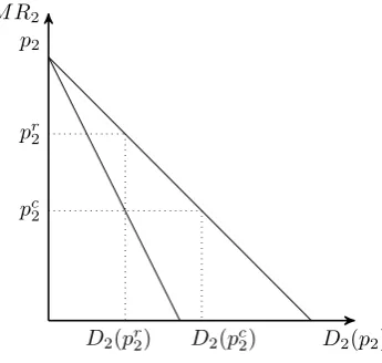
7.3 Forward contracts
In practice, a potentially valuable instrument to which a firm can resort in some markets to restore its commitment powers is a forward or futures contract that specifies the trade of a good at a given price, with delivery and payment occurring at a future point.19 We argue that in our framework forward contracting cannot remove the commitment problem. The presence of buyers that act in the market as arbitrageurs or speculators and are not interested in final
18Applying the framework formalized in the Supplementary Appendix to a three-period model with demand
Dτ =ατ−pτ,τ∈ {1,2,3}, we find that the full commitment prices arepc1= α1+α2+α36+3(c−2sb),pc2=pc1+sband
pc3=pc1+ 2sb. Standard computations yieldM R2(Dc2)−M R3(D3c) =α3−α2−2sb>0, where the inequality
follows from the conditionpm
2 +sb< pm3 (direct extension of Assumption 2
′
in a three-period model).
consumption generates ex post incentives for contract renegotiation between the producer and the buyers. Indeed, forward contracts are rarely executed in reality.
D2(p2)
M R2 p2
pr
2
D2(pr2) pc
2
[image:22.595.212.385.115.279.2]D2(pc2)
Figure 4: Forward contracts
To understand the rationale for this result, consider a contract that commits the producer to deliver to the buyers in the second period a quantity D2(pc2) at a unit price pc2, which
potentially replicates the full commitment solution. If the contract is perfectly enforced, buyers clearly make zero profits, since they resell the good to final consumers at the same price pc2. With the help of Figure 4 we can see that the contract renegotiation in the second period is mutually beneficial. Suppose that a new contract is proposed according to which the producer retains the quantityD2(pr2) < D2(pc2) in exchange for a two-part tariff specifying a unit price
pc2 and a fixed fee. Since the producer can charge a unit price pr2 > pc2 to final consumers, the fixed fee allows the producer to share the resulting gains from trade with the buyers. The residual quantity D2(pc2)−D2(pr2) may be regularly delivered by the producer at pc2 and sold
to final consumers at the same price. The producer is able to engage in price discrimination among final consumers and to increase the second period profits relative to full commitment. Consequently, the full commitment solution collapses.
Notably, the fact that buyers purchase the entire full commitment quantityD2(pc
2) through
forward contracting is irrelevant. Our rationale carries over even when final consumers also participate in the forward market, although this seems less plausible to occur in practice. The crucial point is that the presence of buyers that are not interested in final consumption prevents forward contracts from restoring the full commitment solution.
7.4 Discount factor
framework, the inventory costsp can be interpreted as a measure of the weight on the future in
the firm’s current production and inventory decisions. A lower sp reflects a greater interest in
accumulating inventories for future sales at a higher price. Therefore, our model predicts that the inventories of a producer with a longer business horizon mitigate to a larger extent the loss from the lack of limited commitment. Note that, while the discount factor generally applies to the entire profits, the inventory cost only directly affects the production and inventory activities. Despite this difference, since a higher discount factor makes the producer’s limited commitment problem more significant, we expect that a larger strategic use of inventories will be associated with a higher discount factor (or lower interest rates), analogously to what we find with a lower inventory cost.
The buyer stockpiling cost sb captures the buyer discount factor in an intuitive manner.
The buyer stockpiling behavior affects the producer’s intertemporal problem more prominently when buyers are more forward-looking, namely, the buyer stockpiling cost is lower.
8
Conclusions: managerial, empirical and policy implications
A full understanding of the firms’ inventory behavior is a challenging task that goes well be-yond our study. In this paper, we unveil a strategic channel for inventories that complements the traditional inventory theories. We characterize the producer’s strategic incentives to hold inventories in a dynamic storable good monopoly framework `a la Dudine et al. (2006) where the producer is unable to commit to future prices and forward-looking buyers can stockpile in expectation of higher future prices. Anticipating that the producer cannot refrain from charging a higher future price than under full commitment, buyers engage in wasteful stockpiling. In this setting, we show that the producer’s inventories act as a strategic device to mitigate the loss from the lack of commitment. Since their cost is sunk when being available for sale, inventories reduce future costs, which translates into lower future prices and weakens the buyer stockpiling incentives. When the (unit) cost of production is relatively large, the producer accumulates the level of inventories that maximizes the ex ante profits, and the constraint of sequential optimality is slack in equilibrium. As a result, buyer stockpiling is fully removed, despite the lack of commitment. The only additional cost is the mere inventory cost. When the cost of production is small enough, inventories can be still beneficial for the producer although their amount is distorted from the ex ante optimal level to ensure sequential optimality. This implies that buyer stockpiling can persist in equilibrium. We also provide non-trivial results about the features of equilibrium prices. Although our attention is devoted to storable goods, similar storage incentives apply to durable goods, as Dudine et al. (2006) emphasize. Therefore, the predictions of our model can be extended to durable good markets.