Compressing Neural Language Models by Sparse Word Representations
Yunchuan Chen,1,2 Lili Mou,1,3Yan Xu,1,3 Ge Li,1,3Zhi Jin1,3,∗
1Key Laboratory of High Confidence Software Technologies (Peking University), MoE, China 2University of Chinese Academy of Sciences,[email protected]
3Institute of Software, Peking University,[email protected], {xuyan14,lige,zhijin}@pku.edu.cn ∗Corresponding author
Abstract
Neural networks are among the state-of-the-art techniques for language modeling. Existing neural language models typically map discrete words to distributed, dense vector representations. After information processing of the preceding context words by hidden layers, an output layer estimates the probability of the next word. Such ap-proaches are time- and memory-intensive because of the large numbers of parame-ters for word embeddings and the output layer. In this paper, we propose to com-press neural language models by sparse word representations. In the experiments, the number of parameters in our model in-creases very slowly with the growth of the vocabulary size, which is almost imper-ceptible. Moreover, our approach not only reduces the parameter space to a large ex-tent, but also improves the performance in terms of the perplexity measure.1
1 Introduction
Language models (LMs) play an important role in a variety of applications in natural language processing (NLP), including speech recognition and document recognition. In recent years, neu-ral network-based LMs have achieved signifi-cant breakthroughs: they can model language more precisely than traditional n-gram statistics (Mikolov et al., 2011); it is even possible to gen-erate new sentences from a neural LM, benefit-ing various downstream tasks like machine trans-lation, summarization, and dialogue systems (De-vlin et al., 2014; Rush et al., 2015; Sordoni et al., 2015; Mou et al., 2015b).
1Code released on https://github.com/chenych11/lm
Existing neural LMs typically map a discrete word to a distributed, real-valued vector repre-sentation (called embedding) and use a neural model to predict the probability of each word in a sentence. Such approaches necessitate a large number of parameters to represent the em-beddings and the output layer’s weights, which is unfavorable in many scenarios. First, with a wider application of neural networks in resource-restricted systems (Hinton et al., 2015), such ap-proach is too memory-consuming and may fail to be deployed in mobile phones or embedded sys-tems. Second, as each word is assigned with a dense vector—which is tuned by gradient-based methods—neural LMs are unlikely to learn mean-ingful representations for infrequent words. The reason is that infrequent words’ gradient is only occasionally computed during training; thus their vector representations can hardly been tuned ade-quately.
In this paper, we propose a compressed neural language model where we can reduce the number of parameters to a large extent. To accomplish this, we first represent infrequent words’ embeddings with frequent words’ by sparse linear combina-tions. This is inspired by the observation that, in a dictionary, an unfamiliar word is typically defined by common words. We therefore propose an op-timization objective to compute the sparse codes of infrequent words. The property of sparseness (only 4–8 values for each word) ensures the effi-ciency of our model.
Based on the pre-computed sparse codes, we design our compressed language model as follows. A dense embedding is assigned to each common word; an infrequent word, on the other hand, com-putes its vector representation by a sparse combi-nation of common words’ embeddings. We use the long short term memory (LSTM)-based recur-rent neural network (RNN) as the hidden layer of
our model. The weights of the output layer are also compressed in a same way as embeddings. Consequently, the number of trainable neural pa-rameters is a constant regardless of the vocabulary size if we ignore the biases of words. Even con-sidering sparse codes (which are very small), we find the memory consumption grows impercepti-bly with respect to the vocabulary.
We evaluate our LM on the Wikipedia corpus containing up to 1.6 billion words. During train-ing, we adopt noise-contrastive estimation (NCE) (Gutmann and Hyv¨arinen, 2012) to estimate the parameters of our neural LMs. However, dif-ferent from Mnih and Teh (2012), we tailor the NCE method by adding a regression layer (called ZRegressoion) to predict the normalization factor, which stabilizes the training process. Ex-perimental results show that, our compressed LM not only reduces the memory consumption, but also improves the performance in terms of the per-plexity measure.
To sum up, the main contributions of this paper are three-fold. (1) We propose an approach to rep-resent uncommon words’ embeddings by a sparse linear combination of common ones’. (2) We pro-pose a compressed neural language model based on the pre-computed sparse codes. The memory increases very slowly with the vocabulary size (4– 8 values for each word). (3) We further introduce a ZRegressionmechanism to stabilize the NCE algorithm, which is potentially applicable to other LMs in general.
2 Background
2.1 Standard Neural LMs
Language modeling aims to minimize the joint probability of a corpus (Jurafsky and Martin, 2014). Traditional n-gram models impose a Markov assumption that a word is only depen-dent on previousn−1words and independent of its position. When estimating the parameters, re-searchers have proposed various smoothing tech-niques including back-off models to alleviate the problem of data sparsity.
[image:2.595.358.471.61.175.2]Bengio et al. (2003) propose to use a feed-forward neural network (FFNN) to replace the multinomial parameter estimation inn-gram mod-els. Recurrent neural networks (RNNs) can also be used for language modeling; they are especially capable of capturing long range dependencies in sentences (Mikolov et al., 2010; Sundermeyer et
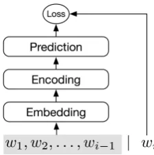
Figure 1: The architecture of a neural network-based language model.
al., 2015).
In the above models, we can view that a neural LM is composed of three main parts, namely the Embedding, Encoding, and Prediction subnets, as shown in Figure 1.
The Embedding subnet maps a word to a dense vector, representing some abstract features of the word (Mikolov et al., 2013). Note that this subnet usually accepts a list of words (known as history or context words) and outputs a sequence of word embeddings.
TheEncodingsubnet encodes the history of a target word into a dense vector (known ascontext
orhistoryrepresentation). We may either leverage FFNNs (Bengio et al., 2003) or RNNs (Mikolov et al., 2010) as theEncodingsubnet, but RNNs typically yield a better performance (Sundermeyer et al., 2015).
The Prediction subnet outputs a distribu-tion of target words as
p(w=wi|h) =Pexp(s(h, wi))
jexp(s(h, wj)), (1)
s(h, wi) =Wi>h+bi, (2)
where h is the vector representation of con-text/historyh, obtained by theEncodingsubnet. W = (W1,W2, . . . ,WV)∈RC×V is theoutput weightsofPrediction;b= (b1, b2, . . . , bV)∈
RC is the bias (the prior). s(h, wi) is a scoring
function indicating the degree to which the context hmatches a target wordwi. (V is the size of
vo-cabularyV;Cis the dimension of context/history, given by theEncodingsubnet.)
2.2 Complexity Concerns of Neural LMs
and the high capacity of Encodingsubnet en-ables complicated information processing.
Despite these, neural LMs also suffer from sev-eral disadvantages mainly out of complexity con-cerns.
Time complexity. Training neural LMs is typi-cally time-consuming especially when the vocab-ulary size is large. The normalization factor in Equation (1) contributes most to time complex-ity. Morin and Bengio (2005) propose hierar-chical softmax by using a Bayesian network so that the probability is self-normalized. Sampling techniques—for example, importance sampling (Bengio and Sen´ecal, 2003), noise-contrastive es-timation (Gutmann and Hyv¨arinen, 2012), and tar-get sampling (Jean et al., 2014)—are applied to avoid computation over the entire vocabulary. In-frequent normalization maximizes the unnormal-ized likelihood with a penalty term that favors nor-malized predictions (Andreas and Klein, 2014).
Memory complexity and model complexity. The number of parameters in the Embedding and Prediction subnets in neural LMs increases linearly with respect to the vocabulary size, which is large (Table 1). As said in Section 1, this is sometimes unfavorable in memory-restricted sys-tems. Even with sufficient hardware resources, it is problematic because we are unlikely to fully tune these parameters. Chen et al. (2015) pro-pose the differentiated softmax model by assign-ing fewer parameters to rare words than to fre-quent words. However, their approach only han-dles the output weights, i.e., W in Equation (2); the input embeddings remain uncompressed in their approach.
In this work, we mainly focus on memory and model complexity, i.e., we propose a novel method to compress theEmbeddingandPrediction subnets in neural language models.
2.3 Related Work
Existing work on model compression for neural networks. Buciluˇa et al. (2006) and Hinton et al. (2015) use a well-trained large network to guide the training of a small network for model compres-sion. Jaderberg et al. (2014) compress neural mod-els by matrix factorization, Gong et al. (2014) by quantization. In NLP, Mou et al. (2015a) learn an embedding subspace by supervised training. Our work resembles little, if any, to the above methods as we compress embeddings and output weights using sparse word representations. Existing model
Sub-nets RNN-LSTM FFNN
Embedding V E V E
Encoding 4(CE+C2+C) nCE+C Prediction V(C+ 1) V(C+ 1) TOTAL† O((C+E)V) O((E+C)V)
Table 1: Number of parameters in different neural network-based LMs. E: embedding dimension; C: context dimension;V: vocabulary size. †Note
thatV C(orE).
compression typically works with a compromise of performance. On the contrary, our model im-proves the perplexity measure after compression.
Sparse word representations. We leverage sparse codes of words to compress neural LMs. Faruqui et al. (2015) propose a sparse coding method to represent each word with a sparse vec-tor. They solve an optimization problem to ob-tain the sparse vectors of words as well as a dic-tionary matrix simultaneously. By contrast, we do not estimate any dictionary matrix when learning sparse codes, which results in a simple and easy-to-optimize model.
3 Our Proposed Model
In this section, we describe our compressed lan-guage model in detail. Subsection 3.1 formal-izes the sparse representation of words, serving as the premise of our model. On such a basis, we compress theEmbeddingandPrediction subnets in Subsections 3.2 and 3.3, respectively. Finally, Subsection 3.4 introduces NCE for pa-rameter estimation where we further propose the ZRegression mechanism to stabilize our model.
3.1 Sparse Representations of Words
We split the vocabularyVinto two disjoint subsets (B andC). The first subset B is a base set, con-taining a fixed number of common words (8k in our experiments).C =V\Bis a set of uncommon words. We would like to useB’s word embeddings to encodeC’s.
com-mon ones’ embeddings. The sparse coefficients are called asparse codefor a given word.
We first train a word representation model like SkipGram (Mikolov et al., 2013) to obtain a set of embeddings for each word in the vocabulary, in-cluding both common words and rare words. Sup-pose U = (U1,U2, . . . ,UB) ∈ RE×B is the
(learned) embedding matrix of common words, i.e.,Uiis the embedding ofi-th word inB. (Here,
B =|B|.)
Each word inB has a natural sparse code (de-noted asx): it is a one-hot vector withBelements, thei-th dimension being on for thei-th word inB. For a wordw∈ C, we shall learn a sparse vector x = (x1, x2, . . . , xB) as the sparse code of the
word. Provided that x has been learned (which will be introduced shortly), the embedding ofwis
ˆ
w= B
X
j=1
xjUj =Ux, (3)
To learn the sparse representation of a certain word w, we propose the following optimization objective
min
x kUx−wk 2
2+αkxk1+β|1>x−1| +γ1>max{0,−x}, (4)
where max denotes the component-wise maxi-mum;wis the embedding for a rare wordw∈ C.
The first term (called fitting loss afterwards) evaluates the closeness between a word’s coded vector representation and its “true” representation w, which is the general goal of sparse coding.
The second term is an`1 regularizer, which
en-courages a sparse solution. The last two regular-ization terms favor a solution that sums to 1 and that is nonnegative, respectively. The nonnegative regularizer is applied as in He et al. (2012) due to psychological interpretation concerns.
It is difficult to determine the hyperparameters α,β, and γ. Therefore we perform several tricks. First, we drop the last term in the problem (4), but clip each element inxso that all the sparse codes are nonnegative during each update of training.
Second, we re-parametrizeα andβ by balanc-ing the fittbalanc-ing loss and regularization terms dy-namically during training. Concretely, we solve the following optimization problem, which is slightly different but closely related to the concep-tual objective (4):
min
x L(x) +αtR1(x) +βtR2(x), (5)
whereL(x) =kUx−wk2
2,R1(x) = kxk1, and
R2(x) =|1>x−1|.αtandβtare adaptive
param-eters that are resolved during training time. Sup-posextis the value we obtain after the update of
thet-th step, we expect the importance of fitness and regularization remain unchanged during train-ing. This is equivalent to
αtR1(xt)
L(xt) =wα ≡const, (6)
βtR2(xt)
L(xt) =wβ ≡const. (7)
or
αt= RL1((xxt)t)wαandβt= RL2((xxt)t)wβ,
wherewαandwβ are the ratios between the
regu-larization loss and the fitting loss. They are much easier to specify thanαorβin the problem (4).
We have two remarks as follows.
• To learn the sparse codes, we first train the “true” embeddings byword2vec2 for both
common words and rare words. However, these true embeddings are slacked during our language modeling.
• As the codes are pre-computed and remain unchanged during language modeling, they are not tunable parameters of our neural model. Considering the learned sparse codes, we need only 4–8 values for each word on av-erage, as the codes contain 0.05–0.1% non-zero values, which are almost negligible.
3.2 Parameter Compression for the
EmbeddingSubnet
One main source of LM parameters is the Embedding subnet, which takes a list of words (history/context) as input, and outputs dense, low-dimensional vector representations of the words.
We leverage the sparse representation of words mentioned above to construct a compressed Embeddingsubnet, where the number of param-eters is independent of the vocabulary size.
By solving the optimization problem (5) for each word, we obtain a non-negative sparse code x ∈ RB for each word, indicating the degree to
which the word is related to common words in B. Then the embedding of a word is given by
ˆ
w=Ux.
We would like to point out that the embedding of a wordwˆis not sparse becauseUis a dense ma-trix, which serves as a shared parameter of learn-ing all words’ vector representations.
3.3 Parameter Compression for the
PredictionSubnet
Another main source of parameters is the Predictionsubnet. As Table 1 shows, the out-put layer contains V target-word weight vectors and biases; the number increases with the vocabu-lary size. To compress this part of a neural LM, we propose a weight-sharing method that uses words’ sparse representations again. Similar to the com-pression of word embeddings, we define a base set of weight vectors, and use them to represent the rest weights by sparse linear combinations.
Without loss of generality, we letD = W:,1:B
be the output weights ofB base target words, and c=b1:Bbe bias of theBtarget words.3 The goal
is to use D and c to represent W and b. How-ever, as the values ofW andbare unknown before the training of LM, we cannot obtain their sparse codes in advance.
We claim that it is reasonable to share the same set of sparse codes to represent word vec-tors in Embedding and the output weights in thePrediction subnet. In a given corpus, an occurrence of a word is always companied by its context. The co-occurrence statistics about a word or corresponding context are the same. As both word embedding and context vectors cap-ture these co-occurrence statistics (Levy and Gold-berg, 2014), we can expect that context vec-tors share the same internal structure as embed-dings. Moreover, for a fine-trained network, given any wordw and its context h, the output layer’s weight vector corresponding to w should spec-ify a large inner-product score for the contexth; thus these context vectors should approximate the weight vector of w. Therefore, word embed-dings and the output weight vectors should share the same internal structures and it is plausible to use a same set of sparse representations for both words and target-word weight vectors. As we shall show in Section 4, our treatment of compressing the Prediction subnet does make sense and achieves high performance.
Formally, thei-th output weight vector is esti-mated by
ˆ
Wi =Dxi, (8) 3W
[image:5.595.325.510.61.223.2]:,1:Bis the firstBcolumns ofW.
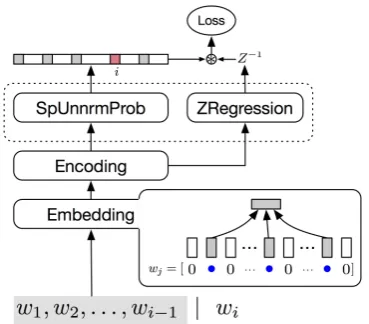
Figure 2: Compressing the output of neural LM. We apply NCE to estimate the parameters of the Predictionsub-network (dashed round rectan-gle). The SpUnnrmProb layer outputs a sparse,
unnormalized probability of the next word. By “sparsity,” we mean that, in NCE, the probability is computed for only the “true” next word (red) and a few generated negative samples.
The biases can also be compressed as
ˆ
bi =cxi. (9)
where xi is the sparse representation of the i-th
word. (It is shared in the compression of weights and biases.)
In the above model, we have managed to com-pressed a language model whose number of pa-rameters is irrelevant to the vocabulary size.
To better estimate a “prior” distribution of words, we may alternatively assign an indepen-dent bias to each word, i.e.,bis not compressed. In this variant, the number of model parameters grows very slowly and is also negligible because each word needs only one extra parameter. Exper-imental results show that by not compressing the bias vector, we can even improve the performance while compressing LMs.
3.4 Noise-Contrastive Estimation with
ZRegression
We adopt the noise-contrastive estimation (NCE) method to train our model. Compared with the maximum likelihood estimation of softmax, NCE reduces computational complexity to a large de-gree. We further propose the ZRegression mechanism to stablize training.
need to compute the unnormalized probability of these positive and negative samples. Interested readers are referred to (Gutmann and Hyv¨arinen, 2012) for more information.
Formally, the estimated probability of the word wiwith history/contexthis
P(w|h;θ) = Z1 hP
0(w i|h;θ)
= Z1
hexp(s(wi, h;θ)), (10)
where θ is the parameters and Zh is a
context-dependent normalization factor. P0(w
i|h;θ) is
the unnormalized probability of the w (given by the SpUnnrmProb layer in Figure 2).
The NCE algorithm suggests to take Zh as
pa-rameters to optimize along with θ, but it is in-tractable for context with variable lengths or large sizes in language modeling. Following Mnih and Teh (2012), we setZh = 1 for allh in the base
model (withoutZRegression).
The objective for each occurrence of con-text/historyhis
J(θ|h) = logP(w P(wi|h;θ)
i|h;θ) +kPn(wi)+ k
X
j=1
logP(w kPn(wj)
j|h;θ) +kPn(wj),
wherePn(w)is the probability of drawing a
nega-tive samplew;kis the number of negative samples that we draw for each positive sample.
The overall objective of NCE is
J(θ) =Eh[J(θ|h)]≈ M1
M
X
i=1
J(θ|hi),
wherehiis an occurrence of the context andMis
the total number of context occurrences.
Although settingZh to 1 generally works well
in our experiment, we find that in certain sce-narios, the model is unstable. Experiments show that when the true normalization factor is far away from 1, the cost function may vibrate. To com-ply with NCE in general, we therefore propose a ZRegressionlayer to predict the normalization constantZh dependent onh, instead of treating it
as a constant.
The regression layer is computed by
Zh−1= exp(WZ>h+bZ),
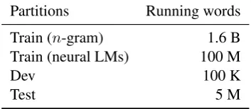
Partitions Running words
Train (n-gram) 1.6 B
Train (neural LMs) 100 M
Dev 100 K
[image:6.595.328.505.65.142.2]Test 5 M
Table 2: Statistics of our corpus.
whereWZ ∈RCandbZ ∈Rare weights and bias
forZRegression. Hence, the estimated proba-bility by NCE withZRegressionis given by
P(w|h) = exp(s(h, w))·exp(W>
Zh+bZ).
Note that the ZRegression layer does not guarantee normalized probabilities. During val-idation and testing, we explicitly normalize the probabilities by Equation (1).
4 Evaluation
In this part, we first describe our dataset in Subsec-tion 4.1. We evaluate our learned sparse codes of rare words in Subsection 4.2 and the compressed language model in Subsection 4.3. Subsection 4.4 provides in-depth analysis of theZRegression mechanism.
4.1 Dataset
We used the freely available Wikipedia4 dump
(2014) as our dataset. We extracted plain sen-tences from the dump and removed all markups. We further performed several steps of preprocess-ing such as text normalization, sentence splittpreprocess-ing, and tokenization. Sentences were randomly shuf-fled, so that no information across sentences could be used, i.e., we did not consider cached language models. The resulting corpus contains about 1.6 billion running words.
The corpus was split into three parts for train-ing, validation, and testing. As it is typically time-consuming to train neural networks, we sampled a subset of 100 million running words to train neu-ral LMs, but the full training set was used to train the backoff n-gram models. We chose hyperpa-rameters by the validation set and reported model performance on the test set. Table 2 presents some statistics of our dataset.
4.2 Qualitative Analysis of Sparse Codes
To obtain words’ sparse codes, we chose 8k com-mon words as the “dictionary,” i.e., B = 8000.
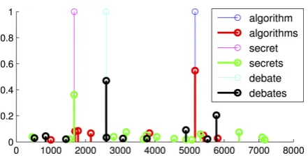
Figure 3: The sparse representations of selected words. Thex-axis is the dictionary of 8k common words; they-axis is the coefficient of sparse cod-ing. Note that algorithm, secret, and debateare common words, each being coded by itself with a coefficient of 1.
We had 2k–42k uncommon words in different set-tings. We first pretrained word embeddings of both rare and common words, and obtained 200d vectorsU andwin Equation (5). The dimension was specified in advance and not tuned. As there is no analytic solution to the objective, we opti-mized it by Adam (Kingma and Ba, 2014), which is a gradient-based method. To filter out small co-efficients around zero, we simply set a value to 0 if it is less than0.015·max{v∈x}.wαin
Equa-tion (6) was set to 1 because we deemed fitting loss and sparsity penalty are equally important. We set wβin Equation (7) to 0.1, and this hyperparameter
is insensitive.
Figure 3 plots the sparse codes of a few selected words. As we see, algorithm,secret, and debate
are common words, and each is (sparsely) coded by itself with a coefficient of 1. We further notice that a rare word likealgorithmshas a sparse rep-resentation with only a few non-zero coefficient.
Moreover, the coefficient in the code of al-gorithms—corresponding to the base word algo-rithm—is large (∼0.6), showing that the words
algorithmandalgorithms are similar. Such phe-nomena are also observed withsecretanddebate. The qualitative analysis demonstrates that our approach can indeed learn a sparse code of a word, and that the codes are meaningful.
4.3 Quantitative Analysis of Compressed Language Models
We then used the pre-computed sparse codes to compress neural LMs, which provides quantita-tive analysis of the learned sparse representations of words. We take perplexity as the performance measurement of a language model, which is
de-fined by
PPL = 2−1
N
PN
i=1log2p(wi|hi)
where N is the number of running words in the test corpus.
4.3.1 Settings
We leveraged LSTM-RNN as theEncoding sub-net, which is a prevailing class of neural networks for language modeling (Sundermeyer et al., 2015; Karpathy et al., 2015). The hidden layer was 200d. We used the Adam algorithm to train our neural models. The learning rate was chosen by valida-tion from{0.001,0.002,0.004,0.006,0.008}. Pa-rameters were updated with a mini-batch size of 256 words. We trained neural LMs by NCE, where we generated 50 negative samples for each pos-itive data sample in the corpus. All our model variants and baselines were trained with the same pre-defined hyperparameters or tuned over a same candidate set; thus our comparison is fair.
We list our compressed LMs and competing methods as follows.
• KN3. We adopted the modified Kneser-Ney smoothing technique to train a 3-gram LM; we used the SRILM toolkit (Stolcke and oth-ers, 2002) in out experiment.
• LBL5. ALog-BiLinear model introduced in Mnih and Hinton (2007). We used 5 preced-ing words as context.
• LSTM-s. A standard LSTM-RNN language model which is applied in Sundermeyer et al. (2015) and Karpathy et al. (2015). We im-plemented the LM ourselves based on Theano (Theano Development Team, 2016) and also used NCE for training.
• LSTM-z. An LSTM-RNN enhanced with theZRegression mechanism described in Section 3.4.
• LSTM-z,wb. Based on LSTM-z, we com-pressed word embeddings in Embedding and the output weights and biases in Prediction.
• LSTM-z,w. In this variant, we did not com-press the bias term in the output layer. For each word inC, we assigned an independent bias parameter.
4.3.2 Performance
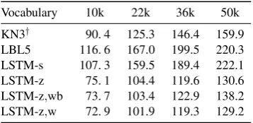
[image:7.595.72.293.57.172.2]Vocabulary 10k 22k 36k 50k KN3† 90. 4 125.3 146.4 159.9 LBL5 116. 6 167.0 199.5 220.3 LSTM-s 107. 3 159.5 189.4 222.1 LSTM-z 75. 1 104.4 119.6 130.6 LSTM-z,wb 73. 7 103.4 122.9 138.2 LSTM-z,w 72. 9 101.9 119.3 129.2
Table 3: Perplexity of our compressed language models and baselines. †Trained with the full
cor-pus of 1.6 billion running words.
[image:8.595.73.291.336.440.2]Vocabulary 10k 22k 36k 50k LSTM-z,w 17.76 59.28 73.42 79.75 LSTM-z,wb 17.80 59.44 73.61 79.95
Table 4: Memory reduction (%) by our proposed methods in comparison with the uncompressed model LSTM-z. The memory of sparse codes are included.
Figure 4: Fine-grained plot of performance (perplexity) and memory consumption (including sparse codes) versus the vocabulary size.
model as well as the backoff 3-gram LM, even if the 3-gram LM is trained on a much larger cor-pus with 1.6 billion words. TheZRegression mechanism improves the performance of LSTM to a large extent, which is unexpected. Subsec-tion 4.4 will provide more in-depth analysis.
Regarding the compression method proposed in this paper, we notice that LSTM-z,wb and LSTM-z,w yield similar performance to LSTM-z. In particular, LSTM-z,w outperforms LSTM-z in all scenarios of different vocabulary sizes. More-over, both LSTM-z,wb and LSTM-z,w can reduce the memory consumption by up to80%(Table 4). We further plot in Figure 4 the model perfor-mance (lines) and memory consumption (bars) in a fine-grained granularity of vocabulary sizes. We see such a tendency that compressed LMs (LSTM-z,wb and LSTM-z,w, yellow and red lines) are generally better than LSTM-z (black line) when
we have a small vocabulary. However, LSTM-z,wb is slightly worse than LSTM-z if the vocabu-lary size is greater than, say, 20k. The LSTM-z,w remains comparable to LSTM-z as the vocabulary grows.
To explain this phenomenon, we may imagine that the compression using sparse codes has two effects: it loses information, but it also enables more accurate estimation of parameters especially for rare words. When the second factor dominates, we can reasonably expect a high performance of the compressed LM.
From the bars in Figure 4, we observe that tra-ditional LMs have a parameter space growing lin-early with the vocabulary size. But the number of parameters in our compressed models does not increase—or strictly speaking, increases at an ex-tremely small rate—with vocabulary.
These experiments show that our method can largely reduce the parameter space with even per-formance improvement. The results also verify that the sparse codes induced by our model indeed capture meaningful semantics and are potentially useful for other downstream tasks.
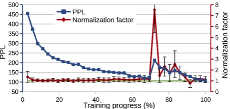
4.4 Effect ofZRegression
We next analyze the effect ofZRegressionfor NCE training. As shown in Figure 5a, the training process becomes unstable after processing 70% of the dataset: the training loss vibrates significantly, whereas the test loss increases.
We find a strong correlation between unsta-bleness and the Zh factor in Equation (10), i.e.,
the sum of unnormalized probability (Figure 5b). Theoretical analysis shows that theZhfactor tends
to be self-normalized even though it is not forced to (Gutmann and Hyv¨arinen, 2012). However, problems would occur, should it fail.
In traditional methods, NCE jointly estimates normalization factor Z and model parameters (Gutmann and Hyv¨arinen, 2012). For language modeling, Zh dependents on context h. Mnih
and Teh (2012) propose to estimate a separateZh
based on two history words (analogous to 3-gram), but their approach hardly scales to RNNs because of the exponential number of different combina-tions of history words.
We propose theZRegressionmechanism in Section 3.4, which can estimate theZhfactor well
(a) Training/test loss vs. training time w/o
ZRegression. (b) The validation perplexity and normalization factorZRegression. Zhw/o
(c) Training loss vs. training time w/
[image:9.595.273.499.68.175.2]ZRegressionof different runs. (d) The validation perplexity and normalization factorZRegression. Zhw/
Figure 5: Analysis ofZRegression.
a large margin, as has shown in Table 3.
It should be mentioned that ZRegressionis not specific to model compression and is generally applicable to other neural LMs trained by NCE.
5 Conclusion
In this paper, we proposed an approach to repre-sent rare words by sparse linear combinations of common ones. Based on such combinations, we managed to compress an LSTM language model (LM), where memory does not increase with the vocabulary size except a bias and a sparse code for each word. Our experimental results also show that the compressed LM has yielded a better per-formance than the uncompressed base LM.
Acknowledgments
This research is supported by the National Ba-sic Research Program of China (the 973 Pro-gram) under Grant No. 2015CB352201, the Na-tional Natural Science Foundation of China under Grant Nos. 61232015, 91318301, 61421091 and 61502014, and the China Post-Doctoral Founda-tion under Grant No. 2015M580927.
References
Jacob Andreas and Dan Klein. 2014. When and why are log-linear models self-normalizing. In Proceed-ings of the Annual Meeting of the North American Chapter of the Association for Computational Lin-guistics, pages 244–249.
Yoshua Bengio and Jean-S´ebastien Sen´ecal. 2003. Quick training of probabilistic neural nets by im-portance sampling. InProceedings of the Ninth In-ternational Workshop on Artificial Intelligence and Statistics.
Yoshua Bengio, R´ejean Ducharme, Pascal Vincent, and Christian Jauvin. 2003. A neural probabilistic lan-guage model. The Journal of Machine Learning Re-search, 3:1137–1155.
Cristian Buciluˇa, Rich Caruana, and Alexandru Niculescu-Mizil. 2006. Model compression. In Proceedings of the 12th ACM SIGKDD Interna-tional Conference on Knowledge Discovery and Data Mining, pages 535–541.
Welin Chen, David Grangier, and Michael Auli. 2015. Strategies for training large vocabulary neural lan-guage models. arXiv preprint arXiv:1512.04906. Jacob Devlin, Rabih Zbib, Zhongqiang Huang, Thomas
Manaal Faruqui, Yulia Tsvetkov, Dani Yogatama, Chris Dyer, and Noah A. Smith. 2015. Sparse overcom-plete word vector representations. In Proceedings of the 53rd Annual Meeting of the Association for Computational Linguistics, pages 1491–1500. Yunchao Gong, Liu Liu, Ming Yang, and Lubomir
Bourdev. 2014. Compressing deep convolutional networks using vector quantization. arXiv preprint arXiv:1412.6115.
Michael Gutmann and Aapo Hyv¨arinen. 2012. Noise-contrastive estimation of unnormalized statistical models, with applications to natural image statis-tics. The Journal of Machine Learning Research, 13(1):307–361.
Zhanying He, Chun Chen, Jiajun Bu, Can Wang, Lijun Zhang, Deng Cai, and Xiaofei He. 2012. Document summarization based on data reconstruction. In Pro-ceedings of the 26th AAAI Conference on Artificial Intelligence, pages 620–626.
Geoffrey Hinton, Oriol Vinyals, and Jeff Dean. 2015. Distilling the knowledge in a neural network. arXiv preprint arXiv:1503.02531.
Max Jaderberg, Andrea Vedaldi, and Andrew Zisser-man. 2014. Speeding up convolutional neural net-works with low rank expansions. InProceedings of the British Machine Vision Conference.
S´ebastien Jean, Kyunghyun Cho, Roland Memisevic, and Yoshua Bengio. 2014. On using very large tar-get vocabulary for neural machine translation. arXiv preprint arXiv:1412.2007.
Dan Jurafsky and James H. Martin. 2014. Speech and Language Processing. Pearson.
Andrej Karpathy, Justin Johnson, and Fei-Fei Li. 2015. Visualizing and understanding recurrent networks. arXiv preprint arXiv:1506.02078.
Diederik P Kingma and Jimmy Ba. 2014. Adam: A method for stochastic optimization. arXiv preprint arXiv:1412.6980.
Honglak Lee, Alexis Battle, Rajat Raina, and An-drew Y Ng. 2006. Efficient sparse coding algo-rithms. InAdvances in Neural Information Process-ing Systems, pages 801–808.
Omer Levy and Yoav Goldberg. 2014. Linguistic reg-ularities in sparse and explicit word representations. InProceedings of the Eighteenth Conference on Nat-ural Language Learning, pages 171–180.
Tomas Mikolov, Martin Karafi´at, Lukas Burget, Jan Cernock`y, and Sanjeev Khudanpur. 2010. Recur-rent neural network based language model. In IN-TERSPEECH, pages 1045–1048.
Tomas Mikolov, Anoop Deoras, Daniel Povey, Lukas Burget, and Jan Cernock´y. 2011. Strategies for training large scale neural network language models.
InProceedings of the IEEE Workshop on Automatic Speech Recognition and Understanding, pages 196– 201.
Tomas Mikolov, Kai Chen, Greg Corrado, and Jef-frey Dean. 2013. Efficient estimation of word representations in vector space. arXiv preprint arXiv:1301.3781.
Andriy Mnih and Geoffrey Hinton. 2007. Three new graphical models for statistical language modelling. InProceedings of the 24th International Conference on Machine learning, pages 641–648.
Andriy Mnih and Yee-Whye Teh. 2012. A fast and simple algorithm for training neural probabilistic language models.arXiv preprint arXiv:1206.6426. Fr´ederic Morin and Yoshua Bengio. 2005.
Hierarchi-cal probabilistic neural network language model. In Proceedings of the International Workshop on Arti-ficial Intelligence and Statistics, pages 246–252. Lili Mou, Ge Li, Yan Xu, Lu Zhang, and Zhi Jin.
2015a. Distilling word embeddings: An encoding approach.arXiv preprint arXiv:1506.04488. Lili Mou, Rui Yan, Ge Li, Lu Zhang, and Zhi Jin.
2015b. Backward and forward language modeling for constrained natural language generation. arXiv preprint arXiv:1512.06612.
Alexander M Rush, Sumit Chopra, and Jason Weston. 2015. A neural attention model for abstractive sen-tence summarization. In Proceedings of the 2015 Conference on Empirical Methods in Natural Lan-guage Processing, pages 379–389.
Alessandro Sordoni, Michel Galley, Michael Auli, Chris Brockett, Yangfeng Ji, Margaret Mitchell, Jian-Yun Nie, Jianfeng Gao, and Bill Dolan. 2015. A neural network approach to context-sensitive gen-eration of conversational responses. In Proceed-ings of the 2015 Conference of the North Ameri-can Chapter of the Association for Computational Linguistics: Human Language Technologies, pages 196–205.
Andreas Stolcke et al. 2002. SRILM—An extensi-ble language modeling toolkit. InINTERSPEECH, pages 901–904.
Martin Sundermeyer, Hermann Ney, and Ralf Schl¨uter. 2015. From feedforward to recurrent LSTM neural networks for language modeling. IEEE/ACM Trans-actions on Audio, Speech and Language Processing, 23(3):517–529.
Theano Development Team. 2016. Theano: A Python framework for fast computation of mathematical ex-pressions. arXiv preprint arXiv:1605.02688. Meng Yang, Lei Zhang, Jian Yang, and David Zhang.