Munich Personal RePEc Archive
Reassignment-proof rules for land rental
problems
Valencia-Toledo, Alfredo and Vidal-Puga, Juan
Universidade de Vigo
3 August 2018
Online at
https://mpra.ub.uni-muenchen.de/92133/
Reassignment-proof rules for land rental
problems
∗
Alfredo Valencia-Toledo
†Juan Vidal-Puga
‡August 3, 2018
Abstract
We consider land rental problems where there are several
communi-ties that can act as lessors and a single tenant who does not necessary need all the available land. A rule should determine which
commu-nities become lessors, how much land they rent and at which price. We present a complete characterization of the family of rules that
sat-isfy reassignment-proofness by merging and spliting, apart from land monotonicity. We also define two parametric subfamilies. The first one is characterized by adding a property of weighted standard for
two-person. The second one is characterized by adding consistency and continuity.
Keywords—land rental, non-manipulability, reassignment-proofness, land monotonicity, consistency.
∗Alfredo Valencia-Toledo thanks the Ministry of Education of Peru for its financial
sup-port through the “Beca Presidente de la Rep´ublica” grant of the “Programa Nacional de Becas y Cr´edito Educativo (PRONABEC)”. Juan Vidal-Puga acknowledges financial sup-port from the Spanish Ministerio de Econom´ıa y Competitividad through grant ECO2014-52616-R., Ministerio de Econom´ıa, Industria y Competitividad through grant ECO2017-82241-R, and Xunta de Galicia (GRC 2015/014).
†Research Group in Economic Analysis (RGEA). Universidade de Vigo, Spain. E-mail:
‡Departamento de Estad´ıstica e IO. Universidade de Vigo, Spain. E-mail:
1
Introduction
The management of land and natural resources is one of the most critical challenges facing developing countries (Kaye and Yahya,2012;van der Ploeg and Rohner, 2012). In particular, natural resource exploitation is an indus-trial activity that has recently been generating conflicts between firms and indigenous communities in many countries in Latin America, Africa and Asia. Examples include Mexico (Tetreault, 2015), Peru (Arellano-Yanguas, 2011;
Fraser,2018), Sierra Leone (Akiwumi,2014), India (Sarkar,2015,2017), Viet-nam (Nguyen et al., 2018) and Indonesia (Welker, 2009). Another examples appear inSosa(2011) andWalter and Urkidi(2015). Another two examples, both in Colombia, arise from a restitution problem where two agents have rights over the land (Jaramillo et al., 2014) and from land aggregating for housing and infrastructure (Kominers and Weyl, 2012), respectively.
In these land conflicts, there exist rights over the land for each side. For the case of mining activities, Article 10 of the United Nations Declaration on the Rights of Indigenous People defined Free Prior and Informed Consent (FPIC) as the principle that indigenous communities have the right to give or withhold its consent to proposed projects that may affect the land they customarily own, occupy or otherwise use (UN, 2007). On the other hand, the mining firm has an investment and a concession over those lands, or, even if a concession has not been granted yet, the firm may have a profit opportunity high enough to make it possible to compensate the land owners in a fair way (Helwege, 2015). In order to solve these land conflicts, it is fundamental for the planner (e.g. the government) to have all the relevant information about both sides.
strategy-proofness literature in the context of cost sharing (Moulin and Shenker,
2001; Sprumont, 2005; G´omez-R´ua and Vidal-Puga, 2011; Ju, 2013; Mass´o et al.,2015), resource allocation (Erlanson and Flores-Szwagrzak, 2015), job scheduling (Moulin,2007,2008), indivisible object allocation (Sun and Yang,
2003; Svensson, 2009; Morimoto and Serizawa, 2015), assigning problems (Kojima and Manea,2010), and taxation problems (Ju and Moreno-Ternero,
2011), among others. Splitting and merging proofness have also been deeply studied in bankruptcy problems where an estate E > 0 should be divided among a set of claimants N with claims given by c ∈ RN. Several authors (O’Neill,1982;Moulin,1987;Chun,1988;de Frutos,1999;Ju,2003; Moreno-Ternero, 2006,2007; Ju et al., 2007) have showed that merging and splitting proofness in bankruptcy problems leads to a proportional share of the estate. See for example Thomson (2003, 2015a).
In this article, we assume that the government or planner seeks to assign a price and amount of land fairly and efficiently, and at the same time, to guarantee non-manipulability by reassignment-proofness. In particular, our work can be seen as part of the theory of mechanism design applied to land rental (see Sen (2007) for an overview and Sarkar (2017) for a more recent contribution). We assume there is a single tenant who can be a mining firm, and several lessors who can be a group of communities. Each community has some available amount of land ci with a reservation price r per unit, that for simplicity we consider equal for all of them. The mining firm needs to rent an optimal amount of adjacent land E, which is a completely divisible object1.
A rule determines, for each land rental problem, a quantity of adjacent land to be rented by each community and a price that the mining firm must pay as a way of compensation.
In order to study rules that guarantee non-manipulability, we propose a version of strategy-proofness such that communities should not find it prof-itable to re-assign the land among them. For instance, asumme we have two
1
lessors, and the first of them may decide to act as two lessors by spliting her land. A rule which considers a fix price per unit of land and an equalitar-ian land share will not satisfy reassigment-proofness, because the first lessor finds it profitable to split her land.
Also, we propose a version of land monotonicity that assures fairness, in the sense that an increase in the quantity of available land affects positively the final profits to both sides.
Our first result is a complete characterization of the family of rules that satisfy these properties. A rule belongs to this family of rules if the price does not depend on the available land and each amount of rented land is proportional. By adding a property inspired by “standard for two-person” in Hart and Mas-Colell (1989), we characterize a parametric subfamily. A rule belongs to this parametric subfamily of rules if, aditionally, the price depends on a parameter. Another property is consistency, that states that the rule should behave in a similar way independently of the number of agents involved. This is a classical property in cooperative games (seevan den Brink et al. (2013) and Huettner (2015) for two recent applications), and it has also been studied in bankruptcy problems (see Thomson (2008, 2015b) and references herein) and cost sharing problems (see for example Albizuri and Zarzuelo(2007) andKoster(2012)). By adding consistency and continuity we characterize another parametric subfamily of rules. The intersection of both parametric subfamilies singles out two particular rules: one of them optimal for the tenant, where the price coincides with to the tenant’s reservation price, and the other optimal for the lessors, where the price coincides with the maximun feasible value.
continu-ity.
2
The model
Let N+ = {1,2, . . .} be the set of potential lessors. Let N = {1,2, . . . , n} be an arbitrary set of lessors, and let S be an arbitrary subset of N. Given
y ∈ RS, we write y(S) = Pi∈Syi. Given x, y ∈ RS, we write x ≤ y when
xi ≤ yi for all i ∈ S. Moreover 0S denotes the vector (0, . . . ,0) ∈ RS. We denote the set of nonnegative real numbers as R+, and the set of positive
real numbers as R++. We denote the set of rational numbers as Q.
Let VN ={{i, j}:i, j ∈N} be the set of all unordered pairs {i, j} over
N. The elements of VN are called edges. A network G over N is a subset of VN. We say that G is a connected network when, for all i, j ∈ N, there exists a sequence of different edges {{is−1, is}}es=1 that satisfy {is−1, is} ∈G
for all s∈ {1,2, . . . , e},i=i0 and j =ie. We denote the set of all connected
networks overN asGN. Given G∈ GN andS ⊂N, we denote the restriction of G toS as GS, i.e. GS ={{i, j} ∈G:i, j ∈S}.
A land rental problem is a tuple (N0, µ, c, r, G) where N0 = {0} ∪N is
the set of agents with 0 the unique tenant and N the set of lessors, µ :
R+ → R is a function that assign to each amount of adjacent land the
tenant’s revenue when that amount is rented, c ∈ RN++ is the vector whose coordinates represent the amount of available land for each lessor, r ∈ R+
is the reservation price per unit of land for lessors, G ∈ GN identifies the lessors whose land is adjacent. Hence, the aggregate welfare when the tenant rents l units of adjacent land is µ(l) + (c(N)−l)r. We normalise µ(0) = 0, and assume that G is a connected network and that there exists a unique
E ∈]0, c(N)] such that µ(E) + (c(N)−E)r is maximum2 on [0, c(N)].3 We
then denote K = µ(E) as the optimal welfare that the agents can obtain. This implies that K > rE, i.e. there exists benefit of cooperation.
2
Sincerc(N) is constant, this condition is equivalent to µ(E)−rE be maximum.
3
Under these conditions, an efficient allocation implies that the amount of rented adjacent land is E and the welfare of the tenant is K. Thus, the only relevant parameters of µare E andK. Furthermore, for convenience we use
N instead of N0. Henceforth, we would be interested in the “efficient land
rental problem”, denoted by (N, K, E, c, r, G). Let L be the set of all land rental problems.
A feasible agreement is a pair (x, p) ∈ R+N ×R+ satisfying x ≤ c and
{i∈N :xi >0} a connected component in G, where xi is the land rented by lessor i ∈ N, and p is the price per unit of land. The set of feasible agreements on a land rental problem L is denoted asAL. Let A=S
L∈LAL
be the set of all potential feasible agreements.
Given (x, p) ∈ AL, the utility for tenant and each lessor i ∈ N are
u0(x, p) =µ(x(N))−px(N) andui(x, p) = (p−r)xi, respectively.
We define a rule as a function ψ : L −→ A that assigns to each prob-lem L = (N, K, E, c, r, G) ∈ L a feasible agreement (x, p) = ψ(L) ∈ AL, satisfying:
(i) x(N) =E;
(ii) for all α, β > 0, p(N, αK, βE, βc,α
βr, G) = α
βp(N, K, E, c, r, G) and
x(N, αK, βE, βc,αβr, G) = βx(N, K, E, c, r, G);
(iii) r ≤p≤ K E.
The first condition (efficiency) says that the amount of land rented is opti-mal. The second condition (scale invariance) says that the final price and the amount of land rented are independent of changes of scale. The third condition (individual rationality) says that the lessors get at least zero (this is implied by r ≤p), and under efficiency, the tenant also gets at least zero (this is implied by p≤ K
E). Under efficiency, the utility of the tenant can be rewritten as u0(x, p) =K−pE.
unique. On the other hand, a rule is lessors-optimal when the price is given byp= K
E. In the latter case, there are many possible payoff allocations when
E < c(N), all of them giving zero to the tenant.
3
Land reassignment and monotonicity
Since there may be no official registration and demarcation of the customary land, the lessors can reach an agreement of reallocating it in order to share extra benefits so created under a rule.
Formally, assume N = (N \S)∪S, where N \S is connected in G and represents the set of lessors that rearrange their land, while S is the set of lessors that do not. Hence, a new land problem arises, withN′ = (N′\S)∪S
as the new set of lessors, so that S =N ∩N′. Moreover, the new connected
network G′ that determines the adjacent lands should be compatible withG
in the sense that GS =G′S and, for all i∈S,
∃j ∈N\S :{i, j} ∈G⇔ ∃j′ ∈N′\S :{i, j′} ∈G′.
In this case, we say that Gand G′ are S-compatible.
For the planner it is not possible to see this customary land situation, and it may be hard to get the outcome that the rule is supposed to attain. In our context manipulation implies that the lessors will benefit by merging or splitting under reallocating their land. Our aim is to fully identify rules that are free from this concern. We formalise this property as follows.
Reassignment-proofness (RP) Given (N, K, E, c, r, G),(N′, K, E, c′, r, G′)∈
L such that ci =c′i for all i∈S =N ∩N′, c(N \S) =c′(N′\S), and
G and G′ are S-compatible, a rule ψ is reassignment-proof if
X
i∈N\S
ui(ψ(N, K, E, c, r, G)) = X i∈N′\S
ui(ψ(N′, K, E, c′, r, G′)).
their land so that the problem becomes (N′, K, E, c′, r, G′). Analogously, if
the left-hand side of expression is larger than the right-hand side and the problem is (N′, K, E, c′, r, G′), then lessors inN′\S can gain by reallocating
their land so that the problem becomes (N, K, E, c, r, G). S is the set of lessors that remain unchanged (S = ∅ is also possible). This property pre-vents lessors from having incentives for merging or splitting by reallocating their land.
The following property says that an increase of the available land, leaving
K and E unaffected, is (weakly) beneficial for everyone involved.
Land Monotonicity (LM) Given (N, K, E, c, r, G),(N, K, E, c′, r, G′)∈ L
with c≤c′ and G⊆G′, a rule ψ island monotonic if
(i) u0(ψ(N, K, E, c, r, G))≤u0(ψ(N, K, E, c′, r, G′)), and
(ii) for eachi∈N,cj =c′j for allj 6=iimpliesui(ψ(N, K, E, c, r, G))≤
ui(ψ(N, K, E, c′, r, G′)).
Under this property, the tenant will be weakly better off when there are more available land. Furthermore, when only one lessor has more available land and the rest of lessors remain unchanged, this lessor will be weakly better off.
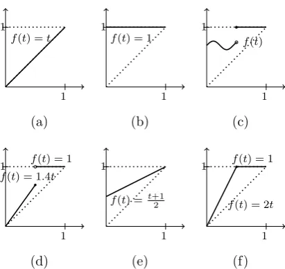
Let F be the set of functions f : [0,1] → [0,1] with f(t) ≥ t for all
t ∈ [0,1]. Now, we consider the family of rules defined by p = K Ef(
rE K) for some f ∈ F and xi = cc(iNE) for all i ∈ N. So, we obtain different rules with different functions f ∈ F. These functions determine the price, whereas the amount of land is always divided proportionally, in line with the known results on invariance under reassignment in cost and surplus sharing (cf. Theorem 1.1 in Moulin (2002)). Figure 1 represents six examples of these functions.
Theorem 3.1 A ruleψ satisfies RP and LM if and only if there existsf ∈ F
such that the price is given by p = K Ef
rE K
1 1
f(t) =t
(a)
1 1
f(t) = 1
(b)
1 1
f(t)
(c)
1 1 f(t) = 1
f(t) = 1.4t
(d)
1 1
f(t) = t+1 2
(e)
1 1 f(t) = 1
f(t) = 2t
[image:10.595.196.402.133.327.2](f)
Figure 1: Examples of functions in F that determine six different rules, including an optimal rule for the tenant (a) and an optimal rule for the lessors (b).
Proof. (⇐) Let ψ be a rule given by p = K Ef
rE K
for some f ∈ F and, when p6= r, xi = cc(iNE) for all i ∈N. We will prove that ψ satisfies RP and LM. In order to prove that ψ satisfies RP, let L = (N, K, E, c, r, G) ∈ L,
L′ = (N′, K, E, c′, r, G′) ∈ L and S = N ∩N′ given as the definition of
RP. Let t = rE
K ∈ [0,1[. On the one hand, we have
P
i∈N\Sui(ψ(L)) =
P
i∈N\S K
Ef(t)−r
ciE
c(N) = K(f(t)−t)
1− cc((NS)). Analogously, on the
other hand, we have Pi∈N′\Sui(ψ(L′)) = K(f(t)−t)
1− cc′′((NS′))
. Since
c(N\S) = c′(N′\S) and c
i =c′i for alli∈S, we have thatc(S) =c′(S) and
c(N) =c′(N′). Hence the last two expressions coincide. We now prove thatψ
satisfies LM. LetLandL′ = (N, K, E, c′, r, G′)∈ Lgiven as in the definition
of LM. Ifc≤c′, then, by efficiency,u
0(ψ(L)) =K−KEf rEK
E =u0(ψ(L′)),
hence condition (i) holds. If ci ≤ c′i and c(N \ {i}) > 0, and cj = c′j for all
j ∈ N \ {i} then ui(ψ(L)) = KEf rEK
−r ciE
c(N) ≤
K Ef
rE K
−r c′iE
c′(N) =
ui(ψ(L′)) for all i∈N, hence condition (ii) also holds.
so on. Furthermore, we write ui instead of ui(x, p), u′i instead of ui(x′, p′) and so on. We proceed by series of claims.
Claim 3.1 If K = E = 1 and N = {1}, then the price p does not depend on c.
Proof. By LM, if c1 ≤ c′1, then u0 ≤ u′0. By efficiency, u0 ≤ u′0 can be
rewritten as 1 −p ≤ 1− p′, hence p ≥ p′ (the higher c
1, the higher p).
Analogously, c1 ≤c′1 implies u1 ≤u′1 and p≤p′ (the higherc1, the lower p).
Therefore, p=p′.
We define f(t) = p({1},1,1,(1), t,∅) for all t ∈ [0,1]. By individual rationality, t≤p({1},1,1,(1), t,∅)≤1 for allt ∈[0,1], so f ∈ F.
Claim 3.2 If K =E = 1, then p=f(r).
Proof. Assume first 1 ∈/ N. By RP, u(N) = u1(ψ({1},1,1,(c(N)), r,∅)).
Under Claim3.1 and efficiency, this is equal top({1},1,1,(1), r,∅)−r, hence
u(N) = f(r)−r. Furthermore, by efficiency,u(N) =Pi∈N(p−r)xi =p−r. Therefore, we havep=f(r). Assume now 1∈N. Leti∈N+\N. Under RP,
ui(ψ({i},1,1,(c(N)), r,∅)) =u1(ψ({1},1,1,(c(N)), r,∅)) and we proceed as
before.
Claim 3.3 p= KEf rEK.
Proof. By scale invariance, p = KEp N,1,1, Ec,rEK, G, and under Claim
3.2 we have thatp= K Ef
rE K
.
Therefore, the price is determined by Claim 3.3. Now we focus on the amount of land x.
Claim 3.4 If p6=r and there exist i, j ∈N such that ci =cj, then xi =xj.
Proof. Fixα ∈N+\N. We define (Niα, K, E, ciα, r, Giα) ∈ L, where Niα =
{i, α}, ciα
i =ci, ciαα =c(N \ {i}), and Giα ={{i, α}}. Since N ∩Niα ={i}, then by RP, u(N \ {i}) = uiα(Niα \ {i}). Under Claim 3.3 and p 6= r, we obtain x(N\ {i}) = xiα
xiα
i +xiαα =E. From these last three equalities we obtain that xi =xiαi . We define (Njα, K, E, cjα, r, Gjα) ∈ L, where Njα ={j, α}, cjα
j =ciαi =ci =cj,
cjα
α =ciαα, andGjα ={{j, α}}. SinceNiα∩Njα ={α}and ciαi =c jα
j , by RP,
ui(xiα, piα) =u
j(xjα, pjα). Under Claim 3.3 and p6=r, we obtainxiαi =x jα j . SinceNjα∩N ={j}and cjα
α =c(N\ {j}), by RP,uα(xjα, pjα) = u(N\ {j}), and under Claim 3.3 and p 6=r, we obtain xjα
α =x(N \ {j}). Furthermore, by efficiency we havexjαj +xjαα =E and xj+x(N\ {j}) =E. So, from these last three equalities we obtain xjαj =xj. Then, fromxi =xiαi , xiαi =x
jα j and
xjαj =xj we get that xi =xj.
Claim 3.5 If N = {i, j}, p 6= r and ci, cj ∈ Q, then xi = cic+iEc
j and xj =
cjE
ci+cj.
Proof. Assume ci = abi
i and cj =
aj
bj where a and b are non-negative integers.
LetNi, Nj ⊂N
+\N withNi∩Nj =∅,|Ni|=aibj and|Nj|=ajbi. We define (N∗i, K, E, c∗i, r, G∗i)∈ L with N∗i =Ni∪ {j} and c∗i
k = bi1bj for all k ∈N
i,
c∗i
j =cj, andG∗i ={{k, j}:k∈Ni}. Since N∩N∗i ={j}andc∗i(N∗i\j) =
ci, by RP, ui = u∗i(N∗i \ {j}). Under Claim 3.3, this is equivalent to write (p−r)xi = (p−r)x∗i(N∗i \ {j}). Since p 6= r, xi = x∗i(N∗i \ {j}). We now define (N∗ij, K, E, c∗ij, r, G∗ij) ∈ Lwith N∗ij = Ni∪Nj, c∗ij
k = bi1bj for
all k ∈ N∗ij, and G∗ij = {{k, k′}:k ∈Ni, k′ ∈Nj}. Since c∗i(N∗i \ {j}) =
c∗ij(N∗ij\Nj),N∗i∩N∗ij =Ni andc∗ij(N∗ij\Ni) = Pajbi
l=1 bi1bj =cj =c ∗i j , by RP, u∗i
j =u∗ij(N∗ij \Ni). Under Claim 3.3, this is equivalent to write (p−
r)x∗i
j = (p−r)x∗ij(N∗ij \Ni). Since p6=r, xj∗i =x∗ij(N∗ij \Ni) = x∗ij(Nj). On the one hand, by efficiency,xi+xj =E andx∗i(N∗i\{j})+x∗ji =E. Since
xi =x∗i(N∗i\{j}) andx∗ji =x∗ij(Nj), we obtainxj =x∗ij(Nj). On the other hand, by efficiency, x∗i(N∗i \ {j}) +x∗i
j = E and x∗ij(Ni) +x∗ij(Nj) = E. Since xi = x∗i(N∗i \ {j}) and x∗ji = x∗ij(Nj), we obtain xi = x∗ij(Ni). We have (N∗ij, K, E, c∗ij, r, G∗ij) with N∗ij ∩N = ∅ and c∗ij(N∗ij) = c(N). By RP, u∗ij(N∗ij) = u(N). By p 6= r and Claim 3.3, this is equivalent to write x∗ij(N∗ij) = x(N). Under Claim 3.4 and efficiency, we obtain that
x∗kij = E
|N∗ij| =
E
aibj+ajbi for all k ∈N
∗ij. By efficiency and x
have that xi = E −x∗ij(Nj). Under Claim 3.4, this is equivalent to write
xi =E−ajbix∗kij for each k∈N∗ij. Sincex∗kij = a E
ibj+ajbi for allk ∈N ∗ij, we
have xi =E − ajbiE
aibj+ajbi =
ciE
ci+cj. Analogously, xj =
cjE
ci+cj.
Claim 3.6 If N ={i, j}, p6=r and cj ∈Q, then xi = cic+iEcj and xj = cjE
ci+cj.
Proof. Assume firstci+cj =E. Then, cciE
i+cj =ciand
cjE
ci+cj =cj. By efficiency,
xi = ci and xj = cj. Therefore, xi = cci+iEcj and xj = cjE
ci+cj. Assume now
ci+cj > E. Let {csi}∞s=1 be a decreasing sequence of rational numbers that
converges to ci. For eachs, we take (N, K, E, cs, r, G)∈ L with cs = (cs i, cj). Under Claim 3.5, we have xs = csiE
cs i+cj,
cjE
cs i+cj
. By LM, ui(x, p) ≤ ui(xs, ps). Under Claim 3.3, this is equivalent to write (p−r)xi ≤ (p− r)xsi. Since
p 6= r, this is equivalent to xi ≤ xsi. Under Claim 3.5, xs = cs
iE
cs i+cj,
cjE
cs i+cj
, which is equivalent to write xi ≤
cs iE
cs
i+cj. Hence, xi ≤
ciE
ci+cj. Let {bc
s
i}∞s=1 be
an increasing sequence of positive rational numbers that converges to ci and such that Lbs = (N, K, E,
b
cs, r, G) ∈ L, where
b
cs = (
b
cs
i, cj). We can find such a sequence because ci > 0 and ci+cj > E. Under Claim 3.5, we have
b
xs = bcs iE
b cs
i+cj,
cjE
b cs
i+cj
. By LM, bus
i ≤ ui. Under Claim 3.3, this is equivalent to write (p−r)xbs
i ≤ (p−r)xi. Since p 6= r, this is equivalent to bxsi ≤ xi. Under Claim 3.5,xbs = bcs
iE
b cs
i+cj,
cjE
b cs
i+cj
, which is equivalent to write bcsiE
b cs
i+cj ≤xi.
Hence, ciE
ci+cj ≤xi. Since xi ≤
ciE
ci+cj and
ciE
ci+cj ≤ xi, we obtain xi =
ciE
ci+cj. By
efficiency, xj =E −xi. Since xi = cciE
i+cj, we deduce xj = E−
ciE
ci+cj =
cjE
ci+cj.
Claim 3.7 If N ={i, j} and p6=r, then xi = cciE
i+cj and xj =
cjE
ci+cj.
Proof. Assume first ci + cj = E. Then, cciE
i+cj = ci and
cjE
ci+cj = cj. By
efficiency, xi =ci and xj =cj. Therefore, xi = cciE
i+cj and xj =
cjE
ci+cj. Assume
nowci+cj > E. Let{csj}∞s=1 a decreasing sequence of rational numbers that
converges to cj. For each s, we take (N, K, E, cs, r, G)∈ Lwith cs= (ci, csj). Under Claim 3.6, we have xs = x
i, cs
jE
ci+csj
. By LM, uj(x, p) ≤ uj(xs, ps). Under Claim 3.3, this is equivalent to write (p−r)xj ≤ (p−r)xsj. Since
p 6= r, this is equivalent to xj ≤xsj = cs
jE
ci+csj. Hence, xj ≤
cjE
ci+cj. Let {bc
be an increasing sequence of rational numbers that converges to cj and such that Lbs = (N, K, E,
b
cs, r, G) ∈ L, where
b
cs = (c
i,bcsj). We can find such a sequence because ci > 0 and ci +cj > E. Under Claim 3.6, we have
b
xs = x i,
b cs
jE
ci+bcsj
. By LM, bus
j ≤ uj. Under Claim 3.3, this is equivalent to write (p−r)bxs
j ≤ (p−r)xj. Since p 6= r, this is equivalent to xbsj ≤ xj, or bc
s jE
ci+bcsj ≤ xj. Hence,
cjE
ci+cj ≤ xj. Since xj ≤
cjE
ci+cj and
cjE
ci+cj ≤ xj, we
obtain xj = cjE
ci+cj. By efficiency, xi = E−xj. Since xj =
cjE
ci+cj, we deduce
xi =E− cjE
ci+cj =
ciE
ci+cj.
Claim 3.8 If p6=r, then xi = cc(iNE) for all i∈N.
Proof. Let i ∈ N, j ∈ N+ \N and (Nij, K, E, cij, r, Gij) ∈ L with Nij = {i, j}, ciji = ci, c
ij
j = c(N \ {i}), and Gij = {{i, j}}. By efficiency, xi =
E − x(N \ {i}). By RP and p 6= r, we have x(N \ {i}) = xijj , so that
xi = E −xijj . Under Claim 3.7, x ij j =
cijjE
ciji +cijj . Hence, xi = E − cijjE ciji +cijj =
E− cc(N\{i})E
i+c(N\{i}) =
ciE
c(N).
Therefore, the amount of land is determined by Claim 3.8.
We denote ψf as the rule corresponding to f ∈ F that is given by p = K
Ef rE
K
, and xi = cc(iNE) for all i∈N.
4
Weighted standard for two-person
We study a property that is inspired on the so called standard for two-person property byHart and Mas-Colell(1989). This property follows a “divide the surplus equally” idea for person situations. In our context, the two-person case arises when |N| = 1, i.e. the only agents are the tenant and a single lessor. Standard for two-person says that both the tenant and the lessor obtain equal benefit. We formalize this property as follows. Let L2 be
the set of land rental problems with a unique lessor.
Standard for 2-person (S2) GivenL= ({1}, K, E, c, r,∅)∈ L2,
Next theorem characterizes the unique rule that satisfies RP, LM and S2. The function that determines this rule is represented in Figure 1(e).
Theorem 4.1 A rule ψ satisfies RP, LM and S2 if and only if the price is given by p= K+rE
2E and the amount of land is given byxi = ciE
c(N) for alli∈N.
Proof. (⇐) Let ψ be a rule given by p = K2+ErE and xi = cc(iNE) for all i ∈N. It is straightforward to check that ψ = ψf with f(t) = 1+t
2 for all t and
p = K+rE
2E . By Theorem 3.1, ψ satisfies RP and LM. So, we just need to prove that u0(ψ({1}, K, E, c, r,∅)) = u1(ψ({1}, K, E, c, r,∅)). The left side
of the equality is equal to K − K+rE
2E E = K−rE
2 . Analogously, the right side
of the equality is equal to K+rE
2E −r
x1. By efficiency, x1 = E, and hence
we obtain u1(ψ({1}, K, E, c, r,∅)) = K−2rE. Therefore, the equality holds.
(⇒) Let ψ be a rule that satisfies RP, LM and S2. By Theorem 3.1
there exists f ∈ F such that p = K Ef
rE K
and, when, p 6= r, xi = cc(iNE) for all i ∈ N. We need to prove that K
Ef rE
K
= K+rE
2E or equivalently
f(t) = 1+t
2 for t =
rE
K ∈ [0,1]. By S2, we have u0(ψ({1},1,1,(1), t,∅)) =
u1(ψ({1},1,1,(1), t,∅)). This is equivalent to 1−f(t)x1 = (f(t)−t)x1. By
efficiency, x1 = 1, which is equivalent to write 1−f(t) = f(t)−t. Hence,
f(t) = 1+t
2 . Finally, since K > rE and c1 = c(N), we deduce p 6= r so
x1 = cc(1NE) =E.
Next, we generalize the standard for two-person concept in a nonsymmet-ric way. Notice that S2 determines the final payoffs for two-person problems, forcing both the tenant and the unique lessor to receive the same value. Since tenant and lessor are not symmetric, we can reasonably allow one side of the market to extract a higher value than the other. In our context, since the rules satisfy efficiency, it is enough to fix the relative payoff between both agents. In particular, a rule satisfies the next property when the payoffs are in the same proportion for every single-lessor problem.
Weighted Standard for 2-person (WS2) There exists ω ∈ [0,1] such that
for all L= ({1}, K, E, c, r,∅)∈ L2.
Next theorem characterizes the parametric subfamily of rules that satisfy RP, LM and WS2. We can see three examples of functions that determine these rules in Figure 1 (a), (b) and (e), respectively.
Theorem 4.2 A ruleψ satisfies RP, LM and WS2 if and only if there exists
ω ∈ [0,1] such that the price is given by p = K−(KE−rE)ω and, when ω < 1, the quantity of land is given by xi = cc(iNE) for all i∈N.
Proof. (⇐) Fixω∈[0,1]. Letψ be a rule given byp= K−(KE−rE)ω and, ifω <
1, then xi = cc(iNE) for all i∈N. By Theorem 3.1, ψ satisfies RP and LM for
f(t) = 1−(1−t)ω and p= K−(KE−rE)ω. Fix L= ({1}, K, E, c, r,∅). We just need to prove that (1−ω)u0(ψ(L)) = ωu1(ψ(L)). The left side of the equality
is equal to (1−ω)K− K−(KE−rE)ωE = (1−ω)ω(K −rE). Analogously, the right side of the equality is equal to ω(K−(KE−rE)ω −r)x1. By efficiency,
x1 =E, and hence the right hand side of the equality is ω(1−ω)(K−rE).
Therefore, equality holds.
(⇒) Let ψ be a rule that satisfies RP, LM and WS2. Let ω ∈[0,1]. By Theorem 3.1, there exists f ∈ F such that p = K
Ef rE
K
and, when p 6= r,
xi = cc(iNE) for all i∈N. This impliesx(N) = E. It is clear thatω <1 implies
p 6= r. To see why, notice that p = r implies u1 = 0, whereas u0 +u1 =
K−rE >0, sou0 >0, and by WS2, (1−ω)u0 =ωu1 = 0, so (1−ω)u0 = 0,
which implies ω = 1. We still need to prove that K Ef
rE K
= K−(KE−rE)ω or, equivalently, f(t) = 1−(1−t)ωfor allt ∈[0,1]. Lett= rE
K ∈[0,1]. By WS2 we have (1 −ω)u0(ψ({1},1,1,(1), t,∅)) = ωu1(ψ({1},1,1,(1), t,∅)). This
is equivalent to (1−ω)(1−f(t)x1) = ω(f(t)−t)x1, which by efficiency is
equivalent to write (1−ω)(1−f(t)) = (f(t)−t)ω. Rearranging terms, we
deduce f(t) = 1−(1−t)ω.
for all t and xi = cc(iNE) for all i ∈ N. In particular, ψ
1
2 is the rule given in
Theorem 4.1.
5
Consistency
Consistency is a well-known principle. Assume that there exists an agreement on what the right price and land share are, and that some lessors take this price and leave. The tenant and the rest of lessors can proceed in two ways: On the one hand, they can keep the previous price and land share. On the other hand, they can recompute the right price and land share following the same principle as before in the new reduced land renting problem. This new reduced land rental problem is defined asL′ = (N′, K′, E′, c′, r, G′)∈ Lgiven
byN′ =N\SwhereS ⊂N is the set of lessors that leave,K′ =K−px(S) is
the new maximal profit of the tenant,E−x(S) is the amount of land that the tenant still needs in the new reduced land rental problem, c′ =c
N\S ∈R N\S
++
is the vector whose coordinates represent the amount of available land, r is the reservation price, which is equal as in the original land rental problem, and G′ identifies the lessors inN′ whose land is adjacent, directly or through
lessors inS. If this procedure always gives the same result for agents inN0\S
as before, we say that ψ is consistent.
Consistency For all (N, K, E, c, r, G) ∈ L and S ⊂ N such that GS is a connected network and x(S)< E, a rule ψ isconsistent if
ui(ψ(N′, K′, E′, c′, r, G′)) =ui(ψ(N, K, E, c, r, G))
for all i ∈ N′
0, where N′ = N \S, K′ = K −px(S), E′ = E−x(S),
c′
i =ci for all i∈N′, and
G′ =G
N′ ∪
n
{i, j} ∈VN′
:∃k, k′ ∈S s.t. {i, k},{j, k′} ∈Go.
Proposition 5.1 A rule ψ satisfies RP, LM and consistency if and only if there exist α, β ∈[0,1] with α ≤β such that:
a) The price is given as follows:
a.1) If r = 0, then either p= 0 or p= K E.
a.2) If r >0 and rE < αK, then p= βαr.
a.3) If r >0 and rE =αK, then p= βαr or p= K E.
a.4) If r >0 and rE > αK, then p= K E.
b) The amount of land when p6=r is given by xi = cc(iNE) for all i∈N.
Proof. (⇐) Let α, β ∈ [0,1] with α ≤ β so that the price and the amount of land are given by a) and b), respectively. Let f ∈ F defined as follows:
f(0) ∈ {0,1}, f(t) = βαt if 0 < t < α, f(α) ∈ {β,1} if α > 0, and f(t) = 1 if t > α. Then, the price can be written as p = K
Ef( rE
K). Hence, by Theorem 3.1, ψ satisfies RP and LM. Let L = (N, K, E, c, r, G) and L′ =
(N′, K′, E′, c′, r, G′) given as in the definition of consistency. We will prove
that ui(x, p) =ui(x′, p′) for all i∈N
0\S, where (x, p) = ψ(L) and (x′, p′) =
ψ(L′). Firstly, we prove that p′ =p. We distinguish the following cases:
Case 1: r= 0 and p= 0. In this case, f(0) = 0. Hence,p′ = 0 and p= 0.
Case 2: r= 0 andp= KE. In this case,f(0) = 1. Hence,p′ = K′
E′. Therefore,
p′ = K′
E′ =
K−K Ex(S)
E−x(S) =
K E =p.
Case 3: r > 0, rE < αK and p = αβr. Under a.2), we know that p′ = β αr when r > 0 and rE′ < αK′. Since r > 0, it is enough to check
that rE′ < αK′. Equivalently, r(E−x(S))< α K− β αrx(S)
. Since
Case 4: r > 0, rE = αK and p = βαr. In this case, p = K
Eβ, so f rE
K
=
β. Since rE′
K′ =
r(E−x(S))
K−K Eβx(S)
= KrE(E(E−−βxx((SS)))) and β ≤ 1, we have that rE′
K′ ≤
rE(E−x(S))
K(E−x(S)) =
rE
K = α. Hence, rE
′ ≤ αK′. We will show that
f rE′
K′
= βαrE′
K′. We have two sub-cases: First, if rE
′ < αK′, then it
holds by a.2) and the fact that p′ = K′
E′f
rE′
K′
. Second, if rE′ = αK′,
then f rE′
K′
= f(α) (rE==αK)f rE K
=β. Since rE′ = αK′, we obtain
that f rEK′′
= αβrEK′′. Hence, p ′ = K′
E′f
rE′
K′
= KE′′
β α
rE′
K′ =
β αr=p
Case 5: r > 0, rE = αK, and p = K
E. Since p = K Ef
rE K
and p = K E, we deduce f rE
K
= 1. Moreover, rE′
K′ =
r(E−x(S))
K−K Ex(S)
= rEK((EE−−xx((SS)))) = rE K =α. Hence, f rE′
K′
= f(α). Since rE = αK and f rE K
= 1, we deduce
f rE′
K′
= 1. Hence, p′ = K′
E′f
rE′
K′
= K′
E′ =
K−K Ex(S)
E−x(S) =
K E =p.
Case 6: rE > αK. In this case, p= K
E. Under a.4), we know that p
′ = K′
E′
when rE′ > αK′. Since K′
E′ =
K−K Ex(S)
E−x(S) =
K
E, it is enough to check that rE′ > αK′. This is equivalent to check that r(E −x(S)) >
α K − K Ex(S)
. Equivalently, r(E−x(S)) > αKE−Ex(S). Since
E−x(S)>0, this is equivalent torE > αK, which is true in this case.
We check now that ui(ψ(L′)) =ui(ψ(L)) for all i∈N0\S. Assume first
i ∈ N \S. We need to prove that (p−r)x′
i = (p−r)xi. This is trivially true when p = r. Hence, assume p 6= r. We need to prove x′
i = xi. Since
c(N) =c(N \S) +c(S), then x′
i = c(Nci\S)(E−x(S)) =
ci
c(N\S)
E −cc((SN)E)=
ci
c(N\S) c
(N)−c(S)
c(N)
E = ci
c(N\S) c
(N\S)
c(N)
E = ci
c(N)E = xi. Assume now i = 0.
We check that u0(ψ(L′)) =u0(ψ(L)), orK′−pE′ =K−pE. By definition,
K′−pE′ = (K−px(S))−p(E−x(S)) =K−pE.
(⇒) Let ψ be a rule that satisfies RP, LM and consistency. Under RP and LM, by Theorem 3.1 there exists f ∈ F such that p = K
Ef rE
K
and, when p6=r, xi = c(cNi)E for all i∈N.
Denote L = (N, K, E, c, r, G) and let S ⊂ N with E > x(S) and L′ =
(N′, K′, E′, c′, r, G′) be defined as in the definition of consistency. Hence,
we have ui(x, p) = ui(x′, p′) for all i ∈ N
(x′, p′) = ψ(L′). In particular, u
0(x, p) = u0(x′, p′). By definition, this is
equivalent to K′−p′E′ =K−pE, or K−px(S)−p′(E−x(S)) =K−pE.
Since E 6=x(S), we deduce p′ =p.
We will prove the existence ofαand β with α≤β, such that the price is given as in a). Or, equivalently,
f(0) ∈ {0,1},
f(t) = β
αt if t ∈]0, α[,
f(α)∈ {β,1} when α >0, and
f(t) = 1 if t > α.
(1)
Iff(t) = 1 for all t∈[0,1], then α= 0 and β = 1 satisfy (1). Hence, we can assume that there existsbtsuch thatf bt <1. Letα=Sup{t:f(t)<1} and β = Sup{f(t) : f(t)< 1}. Then, f(t) ≥ t for all t implies α, β ∈ [0,1] and α ≤β.
For each r ∈[0,1] and γ ∈]0,1[, assume L = ({1,2},1,1,(γ,1−γ), r, G) and S = {2}. So, K′ =K −px
2 = 1−f(r)(1−γ) and E′ = E −x2 = γ.
Hence, we have L′ = ({1},1−f(r)(1−γ), γ,(γ), r,∅).
So, p= K Ef
rE K
=f(r) andp′ = K′
E′f
rE′
K′
= 1−f(rγ)(1−γ)f1−f(rrγ)(1−γ). Since p′ =p, from the last two expressions, we have
f
rγ
1−f(r)(1−γ)
= f(r)γ
1−f(r)(1−γ) for all r∈[0,1] andγ ∈]0,1[. (2)
In particular, for r= 0, we have f(0) = 1−ff(0)(1(0)γ−γ) for all γ. Iff(0) 6= 0, then γ = 1−f(0)(1−γ) for all γ, or equivalently, (1−f(0))γ = 1−f(0) for allγ, which implies thatf(0) = 1. Hencef(0) ∈ {0,1}. This is the first line of (1).
Fort > α, we have f(t) = 1. This is the fourth line of (1). For each r ∈]0,1[, we define Fr(δ) = rδ
1−f(r)(1−δ) ∈ [0, r] for all δ ∈]0,1].
If f(r)<1, then Fr is a strictly increasing and continuous function, and its inverse is given byGr(t) = (1−f(r))t
r−f(r)t ∈]0,1[ for allt ∈]0, r]. Givent∈]0, r] and
f(t) =f(Fr(Gr(t))) =f
rGr(t) 1−f(r)(1−Gr(t))
(2)
= f(r)G r(t) 1−f(r)(1−Gr(t))
= f(r)
(1−f(r))t r−f(r)t
1−f(r)1− (1r−−ff((rr)))tt =
f(r)
r t.
Assume α > 0. Then we can fix r ∈]0,1[ such that f(r) < 1. Hence, f(t)
t = f(r)
r for all t ∈]0, r]. We will prove that f(t) = θt for all t ∈]0, α[, where θ = f(rr). For all t ∈]0, α[, there exists r′ > t such that f(r′) <1 and
f(t)
t = f(r′)
r′ . If t < r, we can taker
′ =r, thus f(t)
t =θ. If t≥ r, then r
′ > r,
thus f(rr) = f(rr′′) =θ. Hence, f(t) = θt for all t ∈]0, α[. We will prove that
θ = αβ, or equivalently rβ =αf(r). We have two cases:
Case I. If f(α) = 1, then β =Sup{f(t) :t ∈]0, α[} =Sup{θt :t ∈]0, α[}=
θα. Hence, θ = βα.
Case II. If f(α) < 1, then f(αα) = θ, so that f(t) = θt for all t ∈]0, α] and
β =Sup{f(t) :t∈]0, α]}=Sup{θt:t∈]0, α]}=θα. Hence, θ = βα.
Then, the second line of (1) is satisfied.
From Case I and Case II we can deduce f(α)∈ {β,1}. This is the third
line of (1).
Given α, β ∈[0,1] with α ≤ β, we define ψα,β as the rule corresponding to the function given in Proposition 5.1 with f(0) = 0, f(α) = β and such that the amount of land is given by xi = cc(iNE) for all i∈N.
Next property says that small changes in the land rental problem should not cause large changes in the chosen allocation.
Continuity The price pand the amount of landx are continuous functions on L.
and it is characterized in the next theorem. We can see some examples of functions that determine these rules in Figure1(a), (b) and (f), respectively.
Theorem 5.1 A rule ψ satisfies RP, LM, consistency and continuity if and only if there exists α∈[0,1] such that:
a)
p=
r
α if rE < αK K
E if rE ≥αK
and
b)
xi =
ciE
c(N) for all i∈N.
Proof. (⇐) Let α ∈[0,1] such that the price and amount of land are given by a) and b) respectively. Part a) can be written as p = K
Ef( rE
K) with
f ∈ F given as f(t) = t
α if t < α and f(t) = 1 if t ≥ α. Hence, by Proposition5.1,ψsatisfies RP, LM and consistency. To prove it that satisfies continuity we still need to check that p is continuous at the points where
rE =αK. Equivalently, limrE→αK+ r
α = K
E, which holds trivially. Moreover,
xi = cc(iNE) for all i∈N also determines a continuous function.
(⇒) Under RP, LM and consistency, by Proposition 5.1there existα, β ∈ [0,1] with α ≤ β such that the price is given as in part a) of Proposition
5.1, and the amount of land whenp6=r, is given by xi = cc(iNE) for all i∈N. By adding continuity, we will prove that p = r
α if rE ≤ αK and p = K E if
rE ≥αK. Moreover, xi = cc(iNE) for all i ∈ N. In this sense, we have that p is a continuous functions in ]0, α[∪]α,1]. We still need to prove the following cases:
i) If r= 0, by continuity, p= limt→0 βαt= 0 = αt.
ii) If rE =αK, by continuity, βαr= K
E. Then,β = Kα
We need to prove that xi = cc(iNE) for all i ∈ N when p = r. Let Lt = (N, K, E, c, rt, G) ∈ L with lim
t→∞rt = 0 and rt > 0 for all t. Therefore,
xt
i = cc(iNE) for all t ∈ [0,1]. Then, under continuity of the land function,
xi = limr→0 cc(iNE) = cc(iNE).
Notice that the functions provided in Theorem 5.1 are those ψα,β with
β = 1. In particular, ψ0,1 = ψ0 (rule ψω when ω = 0) is a rule optimal for the tenant and ψ1 (rule ψω when ω= 1) is a rule optimal for the lessors.
These two rules are the only ones that belong to both parametric sub-families defined at Theorem 4.2 and Theorem 5.1, respectively. Both rules are characterized in the next proposition. We can see the functions that determine these rules in Figure 1 (a) and (b), respectively.
Proposition 5.2 ψ0 and ψ1 are the only rules that satisfy RP, LM, WS2, consistency and continuity.
Proof. It is straightforward to check that both ψ0 andψ1 satisfy these
prop-erties. Let ψ be a rule that satisfies these properties. We will prove that ψ
is either ψ0 or ψ1. On the one hand, by Theorem 5.1, there existsα ∈[0,1]
such that p= K
E whenrE =αK. On the other hand, by Theorem4.2, there exists ω ∈ [0,1] such that p = K−(KE−rE)ω for all r. Hence, given r = αK
E , we have KE = K−(KE−rE)ω, or (K −rE)ω = 0. There are two possibilities: On the one hand, ω = 0 which gives ψ =ψ0. On the other hand, K = rE
and rE = αK imply K =αK. Since K > 0, we deduce α = 1 which gives
ψ =ψ1,1 =ψ1.
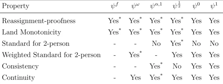
Property ψf ψω ψα,1 ψ1
2 ψ0 ψ1
Reassignment-proofness Yes* Yes* Yes* Yes* Yes Yes
Land Monotonicity Yes* Yes* Yes* Yes* Yes Yes
Standard for 2-person - - No Yes* No No
Weighted Standard for 2-person - Yes* - Yes Yes Yes
Consistency - - Yes* No Yes Yes
[image:24.595.114.483.129.268.2]Continuity - Yes Yes* Yes Yes Yes
Table 1: Summary of the results. Symbol * means that this property, to-gether with others in the same column, characterizes the family/rule.
References
Akiwumi, F. A. (2014). Strangers and Sierra Leone mining: cultural heritage and sustainable development challenges. Journal of Cleaner Production, 84:773–782.
Albizuri, M. J. and Zarzuelo, J. M. (2007). The dual serial cost-sharing rule.
Mathematical Social Sciences, 53(2):150–163.
Arellano-Yanguas, J. (2011). Aggravating the resource curse: Decentralisa-tion, mining and conflict in Peru. The Journal of Development Studies, 47(4):617–638.
Azima, A., Sivapalan, S., Zaimah, R., Suhana, S., and Yusof, H. (2015). Boundry and customary land ownership dispute in Sarawak.Mediterranean Journal of Social Sciences, 6(4).
Chun, Y. (1988). The proportional solution for rights problems.Mathematical Social Sciences, 15(3):231 – 246.
de Frutos, M. A. (1999). Coalitional manipulations in a bankruptcy problem.
Erlanson, A. and Flores-Szwagrzak, K. (2015). Strategy-proof assignment of multiple resources. Journal of Economic Theory, 159, Part A:137 – 162.
Fraser, J. (2018). Mining companies and communities: Collaborative ap-proaches to reduce social risk and advance sustainable development. Re-sources Policy, Forthcoming.
Gildenhuys, J. A. (2005). Indigenous peoples’ rights to minerals and the mining industry: Current developments in South Africa from a national and international perspective.Journal of Energy & Natural Resources Law, 23(4):465–481.
G´omez-R´ua, M. and Vidal-Puga, J. (2011). Merge-proofness in minimum cost spanning tree problems.International Journal of Game Theory, 40(2):309– 329.
Hart, S. and Mas-Colell, A. (1989). Potential, value, and consistency. Econo-metrica, 57(3):589–614.
Helwege, A. (2015). Challenges with resolving mining conflicts in Latin Amer-ica. The Extractive Industries and Society, 2(1):73–84.
Huettner, F. (2015). A proportional value for cooperative games with a coalition structure. Theory and Decision, 78(2):273–287.
Jaramillo, P., Kayı, C¸ ., and Klijn, F. (2014). Asymmetrically fair rules for an indivisible good problem with a budget constraint. Social Choice and Welfare, 43(3):603–633.
Ju, B.-G. (2003). Manipulation via merging and splitting in claims problems.
Review of Economic Design, 8(2):205–215.
Ju, B.-G., Miyagawa, E., and Sakai, T. (2007). Non-manipulable division rules in claim problems and generalizations. Journal of Economic Theory, 132(1):1 – 26.
Ju, B.-G. and Moreno-Ternero, J. (2011). Progressive and merging-proof taxation. International Journal of Game Theory, 40(1):43–62.
Kaye, J. L. and Yahya, M. (2012). Land and Conflict: Tool and guidance for preventing and managing land and natural resources conflict. UN Intera-gency Framework Team for Preventive Action. Guidance Note.
Kojima, F. and Manea, M. (2010). Incentives in the probabilistic serial mechanism. Journal of Economic Theory, 145(1):106 – 123.
Kominers, S. D. and Weyl, E. G. (2012). Holdout in the assembly of comple-ments: A problem for market design. American Economic Review: Papers & Proceedings, 102(3):360–65.
Koster, M. (2012). Consistent cost sharing. Mathematical Methods of Oper-ations Research, 75(1):1–28.
Mass´o, J., Nicol`o, A., Sen, A., Sharma, T., and ¨Ulk¨u, L. (2015). On cost sharing in the provision of a binary and excludable public good. Journal of Economic Theory, 155:30 – 49.
Moreno-Ternero, J. D. (2006). Proportionality and non-manipulability in bankruptcy problems. International Game Theory Review, 8(1):127–139.
Moreno-Ternero, J. D. (2007). Bankruptcy rules and coalitional manipula-tion. International Game Theory Review, 9(2):411–424.
Morimoto, S. and Serizawa, S. (2015). Strategy-proofness and efficiency with non-quasi-linear preferences: a characterization of minimum price Wal-rasian rule. Theoretical Economics, 10(2):445–487.
Moulin, H. (2002). Axiomatic cost and surplus sharing. In Kenneth J. Arrow, A. S. and Suzumura, K., editors, Handbook of Social Choice and Welfare, volume I, chapter 6, pages 289–357. Elsevier.
Moulin, H. (2007). On scheduling fees to prevent merging, splitting, and transferring of jobs. Mathematics of Operations Research, 32(2):266–283.
Moulin, H. (2008). Proportional scheduling, split-proofness, and merge-proofness. Games and Economic Behavior, 63:567–587.
Moulin, H. and Shenker, S. (2001). Strategyproof sharing of submodular costs: budget balance versus efficiency. Economic Theory, 18(3):511–533.
Nguyen, N., Boruff, B., and Tonts, M. (2018). Fool’s gold: Understanding social, economic and environmental impacts from gold mining in quang nam province, vietnam. Sustainability, 10(5):1355–.
O’Neill, B. (1982). A problem of rights arbitration from the Talmud. Math-ematical Social Sciences, 2(4):345 – 371.
Sarkar, S. (2015). Mechanism Design for Land Acquisition. PhD thesis, TERI University.
Sarkar, S. (2017). Mechanism design for land acquisition. International Journal of Game Theory, 46(3):783–812.
Sen, A. (2007). The theory of mechanism design: An overview. Economic and Political Weekly, 42(49):8–13.
Sosa, I. (2011). License to operate: Indigenous relations and free prior and informed consent in the mining industry. Sustainalytics, Amsterdam, The Netherlands.
Sun, N. and Yang, Z. (2003). A general strategy proof fair allocation mech-anism. Economics Letters, 81(1):73–79.
Svensson, L.-G. (2009). Coalitional strategy-proofness and fairness. Eco-nomic Theory, 40(2):227–245.
Tetreault, D. (2015). Social environmental mining conflicts in Mexico. Latin American Perspectives, 42(5):48–66.
Thomson, W. (2003). Axiomatic and game-theoretic analysis of bankruptcy and taxation problems: a survey. Mathematical Social Sciences, 45(3):249 – 297.
Thomson, W. (2008). Two families of rules for the adjudication of conflicting claims. Social Choice and Welfare, 31(4):667–692.
Thomson, W. (2015a). Axiomatic and game-theoretic analysis of bankruptcy and taxation problems: An update. Mathematical Social Sciences, 74:41 – 59.
Thomson, W. (2015b). For claims problems, compromising between the proportional and constrained equal awards rules. Economic Theory, 60(3):495–520.
United Nations (2007). United Nations Declaration on the Rights of Indige-nous Peoples (UNDRIP). Adopted by the General Assembly on 2 October 2007.
van den Brink, R., Funaki, Y., and Ju, Y. (2013). Reconciling marginal-ism with egalitarianmarginal-ism: consistency, monotonicity, and implementation of egalitarian Shapley values. Social Choice and Welfare, 40(3):693–714.
Walter, M. and Urkidi, L. (2015). Community mining consultations in Latin America (2002–2012): The contested emergence of a hybrid institution for participation. Geoforum, In press.