1853
Batch IS NOT Heavy: Learning Word Representations From All Samples
∗Xin Xin1,∗Fajie Yuan1, Xiangnan He2, Joemon M.Jose1 1School of Computing Science, University of Glasgow, UK 2School of Computing, National University of Singapore
{x.xin.1,f.yuan.1}@research.gla.ac.uk, [email protected]
Abstract
Stochastic Gradient Descent (SGD) with negative sampling is the most prevalent approach to learn word representations. However, it is known that sampling meth-ods are biased especially when the sam-pling distribution deviates from the true data distribution. Besides, SGD suffers from dramatic fluctuation due to the one-sample learning scheme. In this work, we propose AllVec that uses batch gradient learning to generate word representations from all training samples. Remarkably, the time complexity of AllVec remains at the same level as SGD, being determined by the number of positive samples rather than all samples. We evaluate AllVec on several benchmark tasks. Experiments show that AllVec outperforms sampling-based SGD methods with comparable ef-ficiency, especially for small training cor-pora.
1 Introduction
Representing words using dense and real-valued vectors, aka word embeddings, has become the cornerstone for many natural language processing (NLP) tasks, such as document classification ( Se-bastiani,2002), parsing (Huang et al.,2012), dis-course relation recognition (Lei et al., 2017) and named entity recognition (Turian et al., 2010). Word embeddings can be learned by optimizing that words occurring in similar contexts have sim-ilar embeddings, i.e. the well-known distribu-tional hypothesis (Harris, 1954). A representa-tive method is skip-gram (SG) (Mikolov et al.,
2013a,b), which realizes the hypothesis using a
∗
The first two authors contributed equally to this paper and share the first-authorship.
[image:1.595.311.535.218.311.2](a) (b)
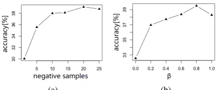
Figure 1: Impact of different settings of negative sampling on skip-gram for the word analogy task on Text8. Clearly, the accuracy depends largely on (a) the sampling size of negative words, and (b) the sampling distribution (β = 0means the uniform distribution andβ = 1means the word frequency distribution).
shallow neural network model. The other family of methods is count-based, such as GloVe ( Pen-nington et al., 2014) and LexVec (Salle et al.,
2016a,b), which exploit low-rank models such as matrix factorization (MF) to learn embeddings by reconstructing the word co-occurrence statistics.
By far, most state-of-the-art embedding meth-ods rely on SGD and negative sampling for opti-mization. However, the performance of SGD is highly sensitive to the sampling distribution and the number of negative samples (Chen et al.,2018;
Yuan et al., 2016), as shown in Figure 1. Es-sentially, sampling is biased, making it difficult to converge to the same loss with all examples, regardless of how many update steps have been taken. Moreover, SGD exhibits dramatic fluc-tuation and suffers from overshooting on local minimums (Ruder, 2016). These drawbacks of SGD can be attributed to its one-sample learning scheme, which updates parameters based on one training sample in each step.
difficulty in applying full batch learning lies in the expensive computational cost for large-scale data. Taking the word embedding learning as an exam-ple, if the vocabulary size is |V|, then evaluating the loss function and computing the full gradient takes O(|V|2k) time, where k is the embedding size. This high complexity is unaffordable in prac-tice, since |V|2 can easily reach billion level or even higher.
In this paper, we introduce AllVec, an exact and efficient word embedding method based on full batch learning. To address the efficiency challenge in learning from all training samples, we devise a regression-based loss function for word embed-ding, which allows fast optimization with memo-rization strategies. Specifically, the acceleration is achieved by reformulating the expensive loss over all negative samples using apartitionand a decou-pleoperation. By decoupling and caching the bot-tleneck terms, we succeed to use all samples for each parameter update in a manageable time com-plexity which is mainly determined by the positive samples. The main contributions of this work are summarized as follows:
• We present a fine-grained weighted least square loss for learning word embeddings. Unlike GloVe, it explicitly accounts for all negative samples and reweights them with a frequency-aware strategy.
• We propose an efficient and exact optimiza-tion algorithm based on full batch gradient optimization. It has a comparable time com-plexity with SGD, but being more effective and stable due to the consideration of all sam-ples in each parameter update.
• We perform extensive experiments on several benchmark datasets and tasks to demonstrate the effectiveness, efficiency, and convergence property of our AllVec method.
2 Related Work
2.1 Skip-gram with Negative Sampling
Mikolov et al. (2013a,b) proposed the skip-gram model to learn word embeddings. SG formulates the problem as a predictive task, aiming at predict-ing the proper contextcfor a target wordwwithin a local window. To speed up the training process, it applies the negative sampling (Mikolov et al.,
2013b) to approximate the full softmax. That is,
each positive (w, c) pair is trained with n ran-domly sampled negative pairs(w, wi). The
sam-pled loss function of SG is defined as
LSGwc = logσ(UwU˜cT)+ n
X
i=1
Ewi∼Pn(w)logσ(−UwU˜wTi)
where Uw and U˜c denote thek-dimensional
em-bedding vectors for wordwand contextc.Pn(w)
is the distribution from which negative contextwi
is sampled.
Plenty of research has been done based on SG, such as the use of prior knowledge from another source (Kumar and Araki,2016;Liu et al.,2015a;
Bollegala et al.,2016), incorporating word type in-formation (Cao and Lu, 2017;Niu et al., 2017), character level n-gram models (Bojanowski et al.,
2016;Joulin et al.,2016) and jointly learning with topic models like LDA (Shi et al.,2017;Liu et al.,
2015b).
2.2 Importance of the Sampling Distribution
Mikolov et al. (2013b) showed that the unigram distribution raised to the 3/4th power as Pn(w)
significantly outperformed both the unigram and the uniform distribution. This suggests that the sampling distribution (of negative words) has a great impact on the embedding quality. Further-more, Chen et al. (2018) and Guo et al. (2018) recently found that replacing the original sam-pler with adaptive samsam-plers could result in bet-ter performance. The adaptive samplers are used to find more informative negative examples dur-ing the traindur-ing process. Compared with the orig-inal word-frequency based sampler, adaptive sam-plers adapt to both the target word and the current state of the model. They also showed that the fine-grained samplers not only speeded up the conver-gence but also significantly improved the embed-ding quality. Similar observations were also found in other fields like collaborative filtering (Yuan et al., 2016). While being effective, it is proven that negative sampling is a biased approximation and does not converges to the same loss as the full softmax — regardless of how many update steps have been taken (Bengio and Sen´ecal,2008;Blanc and Rendle,2017).
2.3 Count-based Embedding Methods
ap-proach in the field of collaborative filtering ( Ko-ren,2008). However, GloVe only formulates the loss on positive entries of the co-occurrence ma-trix, meaning that negative signals about word-context co-occurrence are discarded. A remedy solution is LexVec (Salle et al., 2016a,b) which integrates negative sampling into MF. Some other methods (Li et al., 2015; Stratos et al., 2015;
Ailem et al., 2017) also use MF to approximate the word-context co-occurrence statistics. Al-though predictive models and count-based models seem different at first glance,Levy and Goldberg
(2014) proved that SG with negative sampling is implicitly factorizing a shifted pointwise mutual information (PMI) matrix, which means that the two families of embedding models resemble each other to a certain degree.
Our proposed method departs from all above methods by using the full batch gradient optimizer to learn from all (positive and negative) samples. We propose a fast learning algorithm to show that such batch learning is not “heavy” even with tens of billions of training examples.
3 AllVec Loss
In this work, we adopt the regression loss that is commonly used in count-based models ( Penning-ton et al.,2014;Stratos et al.,2015;Ailem et al.,
2017) to perform matrix factorization on word co-occurrence statistics. As highlighted, to retain the modeling fidelity, AllVec eschews using any sam-pling but optimizes the loss on all positive and negative word-context pairs.
Given a word w and a symmetric window of wincontexts, the set of positive contexts can be obtained by sliding through the corpus. Letc de-note a specific context,Mwcbe the number of
co-occurred(w, c)pairs in the corpus within the win-dow.Mwc= 0means that the pair(w, c)has never
been observed, i.e. the negative signal. rwc is the
association coefficient betweenwandc, which is calculated fromMwc. Specifically, we userwc+ to
denote the ground truth value for positive (w, c)
pairs and a constant valuer−(e.g., 0 or -1) for neg-ative ones since there is no interaction betweenw andc in negative pairs. Finally, with all positive and negative pairs considered, a regular loss func-tion can be given as Eq.(1), whereV is the vocab-ulary andS is the set of positive pairs. α+wc and αwc− represent the weight for positive and negative
(w, c)pairs, respectively.
L= X
(w,c)∈S
α+wc(r +
wc−UwU˜cT) 2
| {z }
LP
+ X
(w,c)∈(V×V)\S
α−wc(r −
−UwU˜cT) 2
| {z }
LN
(1)
When it comes torwc+, there are several choices. For example, GloVe applies the log ofMwc with
bias terms for w andc. However, research from
Levy and Goldberg (2014) showed that the SG model with negative sampling implicitly factorizes a shifted PMI matrix. The PMI value for a(w, c)
pair can be defined as
P M Iwc=log
P(w, c)
P(w)P(c) =log
MwcM∗∗
Mw∗M∗c
(2)
where ‘*’ denotes the summation of all corre-sponding indexes (e.g., Mw∗=Pc∈V Mwc).
In-spired by this connection, we setrwc+ as the posi-tive point-wise mutual information (PPMI) which has been commonly used in the NLP literature (Stratos et al., 2015;Levy and Goldberg, 2014). Sepcifically, PPMI is the positive version of PMI by setting the negative values to zero. Finally,r+wc is defined as
r+wc=P P M Iwc= max(P M Iwc,0) (3)
3.1 Weighting Strategies
Regarding α+wc, we follow the design in GloVe, where it is defined as
α+wc=
(
(Mwc/xmax)ρ Mwc< xmax
1 Mwc≥xmax
(4)
fre-quency, and a smaller weight for infrequent words. Formally,α−wcis defined as
α−wc =α−c =α0 M
δ ∗c
P
c∈V M∗cδ
(5)
whereα0can be seen as a global weight to control the overall importance of negative samples. α0 =
0means that no negative information is utilized in the training. The exponentδis used for smoothing the weights. Specially, δ = 0 means a uniform weight for all negative examples andδ= 1means that no smoothing is applied.
4 Fast Batch Gradient Optimization
Once specifying the loss function, the main chal-lenge is how to perform an efficient optimization for Eq.(1). In the following, we develop a fast batch gradient optimization algorithm that is based on apartitionreformulation for the loss and a de-coupleoperation for the inner product.
4.1 Loss Partition
As can be seen, the major computational cost in Eq.(1) lies in the term LN, because the size of
(V×V)\Sis very huge, which typically contains over billions of negative examples. To this end, we show our first key design that separates the loss of negative samples into the difference between the loss on all samples and that on positive samples1. The loss partition serves as the prerequisite for the efficient computation of full batch gradients.
LN=
X
w∈V
X
c∈V
α−c(r −
−UwU˜cT) 2
−X
(w,c)∈S
α−c(r −
−UwU˜cT) 2
(6)
By replacingLN in Eq.(1) with Eq.(6), we can
ob-tain a new loss function with a more clear struc-ture. We further simplify the loss function by merging the terms on positive examples. Finally, we achieve a reformulated loss
L= X
w∈V
X
c∈V
α−c(r −
−UwU˜cT) 2
| {z }
LA
+ X
(w,c)∈S
(α+wc−α −
c)(∆−UwU˜cT) 2
| {z }
L
P0
+C (7)
where ∆ = (α+wcr+wc−α−cr−)/(α+wc −α−c). It can be seen that the new loss function consists of two components: the lossLAon the wholeV ×V
training examples andLP0 on positive examples.
The major computation now lies inLAwhich has
1The idea here is similar to that used in (He et al.,2016; Li et al.,2016) for a different problem.
a time complexity ofO(k|V|2). In the following, we show how to reduce the huge volume of com-putation by a simple mathematical decouple.
4.2 Decouple
To clearly show the decouple operation, we rewrite LA as LeA by omitting the constant term α−c(r−)2. Note that uwd andu˜cd denote the d-th
element inUwandU˜c, respectively.
e
LA=
X
w∈V
X
c∈V
α−c k
X
d=0
uwdu˜cd k
X
d0=0
uwd0u˜cd0
−2r−X
w∈V
X
c∈V
α−c k
X
d=0
uwdu˜cd
(8)
Now we show our second key design that is based on adecouplemanipulation for the inner product operation. Interestingly, we observe that the sum-mation operator and elements in Uw andU˜c can
be rearranged by the commutative property (Dai et al.,2007), as shown below.
e
LA= k
X
d=0 k
X
d0=0
X
w∈V
uwduwd0
X
c∈V
α−cu˜cdu˜cd0
−2r−
k X d=0 X w∈V uwd X c∈V
α−cu˜cd
(9)
An important feature in Eq.(9) is that the original inner product terms are disappeared, while in the new equationP
c∈V αc−u˜cdu˜cd0 andPc∈V αc−u˜cd
are “constant” values relative to uwduwd0 and
uwd respectively. This means that they can be
pre-calculated before training in each iteration. Specifically, we definepw
dd0,pcdd0,qdwandqdcas the
pre-calculated terms
pwdd0=
X
w∈V
uwduwd0 qwd =
X
w∈V
uwd
pcdd0=
X
c∈V
α−cu˜cdu˜cd0 qdc=
X
c∈V
α−cu˜cd
(10)
Then the computation ofL˜A can be simplified to
Pk
d=0 Pk
d0=0pwdd0pcdd0 −2r−qdwqdc.
It can be seen that the time complexity to com-pute allpwdd0 isO(|V|k2), and similarly,O(|V|k2)
forpcdd0andO(|V|k)forqdwandqdc. With all terms
pre-calculated before each iteration, the time com-plexity of computingL˜Ais justO(k2). As a result,
the total time complexity of computingLA is
de-creased toO(2|V|k2+ 2|V|k+k2)≈O(2|V|k2), which is much smaller than the originalO(k|V|2). Moreover, it’s worth noting that our efficient com-putation for L˜A is strictly equal to its original
value, which means AllVec does not introduce any approximation in evaluating the loss function.
uwdandu˜cdas
∂L ∂uwd
=
k
X
d0=0
uwd0pcdd0−
X
c∈Iw+
Λ·˜ucd−r −
qdc
∂L ∂u˜cd
=
k
X
d0=0 ˜
ucd0pwdd0α−c−
X
w∈I+ c
Λ·uwd−r −
α−cq w d
(11)
whereIw+ denotes the set of positive contexts for w,Ic+denotes the set of positive words for cand
Λ = (α+
wc−α−c)(∆−UwU˜cT). Algorithm 1 shows
the training procedure of AllVec.
Algorithm 1AllVec learning
Input: corpusΓ,win,α0,δ,iter, learning rateη
Output: embedding matricesU andU˜ 1: Build vocabulary V fromΓ
2: Obtain all positive(w, c)andMwcfromΓ
3: Compute allr+wc,α+wcandα−c 4: InitializeU andU˜
5: fori= 1, ..., iterdo 6: ford∈ {0, .., k}do
7: Compute and storeqdc .O(|V|k)
8: ford0 ∈ {0, .., k}do
9: Compute and storepcdd0 .O(|V|k2)
10: end for
11: end for 12: forw∈V do
13: ComputeΛ .O(|S|k)
14: ford∈ {0, .., k}do
15: Updateuwd .O(|S|k+|V|k2)
16: end for
17: end for
18: Repeat 6-17 foru˜cd .O(2|S|k+2|V|k2)
19: end for
4.3 Time Complexity Analysis
In the following, we show that AllVec can achieve the same time complexity with negative sampling based SGD methods.
Given the sample size n, the total time com-plexity for SG is O((n+ 1)|S|k), where n+ 1
denotesnnegative samples and 1 positive exam-ple. Regarding the complexity of AllVec, we can see that the overall complexity of Algorithm 1 is O(4|S|k+ 4|V|k2).
For the ease of discussion, we denote c as the average number of positive contexts for a word in the training corpus, i.e. |S| = c|V|(c ≥ 1000in most cases). We then obtain the ratio
4|S|k+ 4|V|k2
(n+ 1)|S|k =
4
n+ 1(1 +
k
c) (12)
wherekis typically set from 100 to 300 (Mikolov et al.,2013a;Pennington et al.,2014), resulting in k ≤ c. Hence, we can give the lower and upper bound for the ratio:
4
n+1<
4|S|k+4|V|k2
(n+1)|S|k =
4
n+1(1+
k c)≤
8
n+1 (13)
The above analysis suggests that the complexity of AllVec is same as that of SGD with negative sample size between 3 and 7. In fact, considering thatcis much larger thank in most datasets, the major cost of AllVec comes from the part 4|S|k (see Section 5.4 for details), which is linear with respect to the number of positive samples.
5 Experiments
We conduct experiments on three popular evalua-tion tasks, namely word analogy (Mikolov et al.,
2013a), word similarity (Faruqui and Dyer,2014) and QVEC (Tsvetkov et al.,2015).
Word analogy task. The task aims to answer questions like, “ais tobascis to ?”. We adopt the Google testbed2 which contains 19,544such questions in two categories: semantic and syntac-tic. The semantic questions are usually analogies about people or locations, like “king is to man as queen is to ?”, while the syntactic questions fo-cus on forms or tenses, e.g., “swimming is to swim as running to ?”.
Word similarity tasks. We perform evalua-tion on six datasets, including MEN (Bruni et al.,
2012), MC (Miller and Charles,1991), RW ( Lu-ong et al., 2013), RG (Rubenstein and Good-enough, 1965), WS-353 Similarity (WSim) and Relatedness (WRel) (Finkelstein et al., 2001). We compute the spearman rank correlation be-tween the similarity scores calculated based on the trained embeddings and human labeled scores.
QVEC. QVEC is an intrinsic evaluation met-ric of word embeddings based on the alignment to features extracted from manually crafted lexi-cal resources. QVEC has shown strong correlation with the performance of embeddings in several se-mantic tasks (Tsvetkov et al.,2015).
We compare AllVec with the following word embedding methods.
• SG: This is the original skip-gram model with SGD and negative sampling (Mikolov et al.,
2013a,b).
• SGA: This is the skip-gram model with an adaptive sampler (Chen et al.,2018).
Table 1: Corpora statistics.
Corpus Tokens Vocab Size
Text8 17M 71K 100M
NewsIR 78M 83K 500M
Wiki-sub 0.8B 190K 4.0G Wiki-all 2.3B 200K 13.4G
• GloVe: This method applies biased MF on the positive samples of word co-occurrence matrix (Pennington et al.,2014).
• LexVec: This method applies MF on the PPMI matrix. The optimization is done with negative sampling and mini-batch gradient descent (Salle et al.,2016b).
For all baselines, we use the original implementa-tion released by the authors.
5.1 Datasets and Experimental Setup
We evaluate the performance of AllVec on four real-world corpora, namely Text83, NewsIR4, Wiki-sub and Wiki-all. Wiki-sub is a subset of 2017 Wikipedia dump5. All corpora have been pre-processed by a standard pipeline (i.e. remov-ing non-textual elements, lowercasremov-ing and tok-enization). Table 1 summarizes the statistics of these corpora.
To obtainMwcfor positive(w, c)pairs, we
fol-low GloVe where word pairs that arexwords apart contribute1/xtoMwc. The window size is set as
win = 8. Regarding α+wc, we setxmax = 100
andρ = 0.75. For a fair comparison, the embed-ding size k is set as 200 for all models and cor-pora. AllVec can be easily trained by AdaGrad (Zeiler,2012) like GloVe or Newton-like (Bayer et al., 2017; Bradley et al., 2011) second order methods. For models based on negative sampling (i.e. SG, SGA and LexVec), the sample size is set as n = 25 for Text8, n = 10 for NewsIR and n = 5for Wiki-sub and Wiki-all. The setting is also suggested by Mikolov et al. (2013b). Other detailed hyper-parameters are reported in Table2.
5.2 Accuracy Comparison
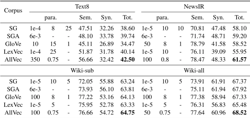
We present results on the word analogy task in Table 2. As shown, AllVec achieves the high-est total accuracy (Tot.) in all corpora,
particu-3
http://mattmahoney.net/dc/text8.zip 4
http://research.signalmedia.co/newsir16/signal-dataset.html
5https://dumps.wikimedia.org/enwiki/
larly in smaller corpora (Text8 and NewsIR). The reason is that in smaller corpora the number of positive (w, c) pairs is very limited, thus making use of negative examples will bring more benefits. Similar reason also explains the poor accuracy of GloVe in Text8, because GloVe does not consider negative samples. Even in the very large corpus (Wiki-all), ignoring negative samples still results in sub-optimal performance.
Our results also show that SGA achieves better performance than SG, which demonstrates the im-portance of a good sampling strategy. However, regardless what sampler (except the full softmax sampling) is utilized and how many updates are taken, sampling is still a biased approach. AllVec achieves the best performance because it is trained on the whole batch data for each parameter update rather than a fraction of sampled data.
Another interesting observation is AllVec per-forms better in semantic tasks in general. The rea-son is that our model utilizes global co-occurrence statistics, which capture more semantic signals than syntactic signals. While both AllVec and GloVe use global contexts, AllVec performs much better than GloVe in syntactic tasks. We argue that the main reason is because AllVec can dis-till useful signals from negative examples, while GloVe simply ignores all negative information. By contrast, local-window based methods, such as SG and SGA, are more effective to capture local sentence features, resulting in good perfor-mance on syntactic analogies. However,Rekabsaz et al.(2017) argues that these local-window based methods may suffer from the topic shifting issue.
Table3and Table4provide results in the word similarity and QVEC tasks. We can see that Al-lVec achieves the best performance in most tasks, which admits the advantage of batch learning with all samples. Interestingly, although GloVe per-forms well in semantic analogy tasks, it shows extremely worse results in word similarity and QVEC. The reason shall be the same as that it per-forms poorly in syntactic tasks.
5.3 Impact ofα−c
Table 2: Results (“Tot.” denotes total accuracy) on the word analogy task.
Corpus Text8 NewsIR
para. Sem. Syn. Tot. para. Sem. Syn. Tot.
SG 1e-4 8 25 47.51 32.26 38.60 1e-5 10 10 70.81 47.48 58.10 SGA 6e-3 - - 48.10 33.78 39.74 6e-3 - - 71.74 48.71 59.20 GloVe 10 15 1 45.11 26.89 34.47 50 8 1 78.79 41.58 58.52 LexVec 1e-4 25 - 51.87 31.78 40.14 1e-5 10 - 76.11 39.09 55.95 AllVec 350 0.75 - 56.66 32.42 42.50 100 0.8 - 78.47 48.33 61.57
Wiki-sub Wiki-all
SG 1e-5 10 5 72.05 55.88 63.24 1e-5 10 5 73.91 61.91 67.37 SGA 6e-3 - - 73.93 56.10 63.81 6e-3 - - 75.11 61.94 67.92 GloVe 100 8 1 77.22 53.16 64.13 100 8 1 77.38 58.94 67.33 LexVec 1e-5 5 - 75.95 52.78 63.33 1e-5 5 - 76.31 56.83 65.48 AllVec 100 0.75 - 76.66 54.72 64.75 50 0.75 - 77.64 60.96 68.52
The parameter columns (para.) for each model are given from left to right as follows. SG: subsampling of frequent words, window size and the number of negative samples; SGA:λ(Chen et al.,2018) that controls the distribution of the rank, the other parameters are the same with SG; GloVe:xmax, window size and symmetric window; LexVec: subsampling of frequent words and the number of negative samples; AllVec: the negative weightα0andδ. Boldface denotes the highest
total accuracy.
Figure 2(a) shows the impact of the overall weightα0by settingδas 0.75 (inspired by the set-ting of skip-gram). Clearly, we observe that all results (including semantic, syntactic and total ac-curacy) have been greatly improved whenα0 in-creases from 0 to a larger value. As mentioned before, α0 = 0 means that no negative informa-tion is considered. This observainforma-tion verifies that negative samples are very important for learning good embeddings. It also helps to explain why GloVe performs poorly on syntactic tasks. In addi-tion, we find that in all corpora the optimal results are usually obtained when α0 falls in the range of 50 to 400. For example, in the NewIR corpus as shown, AllVec achieves the best performance whenα0 = 100. Figure2(b)shows the impact of δwithα0= 100. As mentioned before,δ = 0 de-notes a uniform value for all negative words and δ = 1 denotes that no smoothing is applied to word frequency. We can see that the total accuracy is only around 55% when δ = 0. By increasing its value, the performance is gradually improved, achieving the highest score whenδ is around 0.8. Further increase ofδ will degrade the total accu-racy. This analysis demonstrates the effectiveness of the proposed negative weighting scheme.
5.4 Convergence Rate and Runtime
Figure 3(a) compares the convergence between AllVec and GloVe on NewsIR. Clearly, AllVec
ex-(a) (b)
Figure 2: Effect ofα0andδon NewsIR.
(a) (b)
Figure 3: Convergence and runtime.
hibits a more stable convergence due to its full batch learning. In contrast, GloVe has a more dramatic fluctuation because of the one-sample learning scheme. Figure3(b) shows the relation-ship between the embedding size k and runtime on NewsIR. Although the analysis in Section 4.3 demonstrates that the time complexity of AllVec is O(4|S|k+ 4|V|k2), the actual runtime shows a near linear relationship withk. This is because
4|V|k2/4|S|k = k/c, where c generally ranges from 1000 ∼6000 and kis set from 200 to 300 in practice. The above ratio explains the fact that
[image:7.595.308.535.346.575.2]Table 3: Results on the word similarity task.
Corpus Text8 NewsIR
MEN MC RW RG WSim WRel MEN MC RW RG WSim WRel
SG .6868 .6776 .3336 .6904 .7082 .6539 .7293 .7328 .3705 .7184 .7176 .6147 SGA .6885 .6667 .3399 .7035 .7291 .6708 .7409 .7513 .3797 .7508 .7442 .6398 GloVe .4999 .3349 .2614 .3367 .5168 .5115 .5839 .5637 .2487 .6284 .6029 .5329 LexVec .6660 .6267 .2935 .6076 .7005 .6862 .7301 .8403 .3614 .8341 .7404 .6545
AllVec .6966 .6975 .3424 .6588 .7484 .7002 .7407 .7642 .4610 .7753 .7453 .6322
Wiki-sub Wiki-all
[image:8.595.322.509.314.395.2]SG .7532 .7943 .4250 .7555 .7627 .6563 .7564 .8083 .4311 .7678 .7662 .6485 SGA .7465 .7983 .4296 .7623 .7715 .6560 .7577 .7940 .4379 .7683 .7110 .6488 GloVe .6898 .6963 .3184 .7041 .6669 .5629 .7370 .7767 .3197 .7499 .7359 .6336 LexVec .7318 .7591 .4225 .7628 .7292 .6219 .7256 .8219 .4383 .7797 .7548 .6091 AllVec .7155 .8305 .4667 .7945 .7675 .6459 .7396 .7840 .4966 .7800 .7492 .6518
Table 4: Results on QVEC.
Qvec Text8 NewsIR Wiki-sub Wiki-all
SG .3999 .4182 .4280 .4306 SGA .4062 .4159 .4419 .4464 GloVe .3662 .3948 .4174 .4206 LexVec .4211 .4172 .4332 .4396 AllVec .4211 .4319 .4351 .4489
withkand|S|.
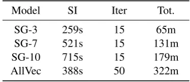
We also compare the overall runtime of AllVec and SG on NewsIR and show the results in Table
5. As can be seen, the runtime of AllVec falls in the range of SG-3 and SG-7 in a single iteration, which confirms the theoretical analysis in Section 4.3. In contrast with SG, AllVec needs more itera-tions to converge. The reason is that each parame-ter in SG is updated many times during each iparame-ter- iter-ation, although only one training example is used in each update. Despite this, the total run time of AllVec is still in a feasible range. Assuming the convergence is measured by the number of param-eter updates, our AllVec yields a much faster con-vergence rate than the one-sample SG method.
In practice, the runtime of our model in each it-eration can be further reduced by increasing the number of parallel workers. Although baseline methods like SG and GloVe can also be paral-lelized, the stochastic gradient steps in these meth-ods unnecessarily influence each other as there is no exact way to separate these updates for differ-ent workers. In other words, the parallelization of SGD is not well suited to a large number of
work-Table 5: Comparison of runtime.
Model SI Iter Tot.
SG-3 259s 15 65m
SG-7 521s 15 131m
SG-10 715s 15 179m
AllVec 388s 50 322m
SG-nrepresentsnnegative samples for skip-gram, SI represents the runtime for a single iteration, and Tot. denotes the total runtime. All models are of embedding size 200 and trained with 8 threads.
ers. In contrast, the parameter updates in AllVec are completely independent of each other, there-fore AllVec does not have the update collision is-sue. This means we can achieve the embarrassing parallelization by simply separating the updates by words; that is, letting different workers update the model parameters for disjoint sets of words. As such, AllVec can provide a near linear scaling without any approximation since there is no poten-tial conflicts between updates.
6 Conclusion
our proposed all-sample learning scheme to deep learning methods, which are more expressive than the shallow embedding model. Moreover, we will integrate prior knowledge, such as the words that are synonyms and antonyms, into the word em-bedding process. Lastly, we are interested in ex-ploring the recent adversarial learning techniques to enhance the robustness of word embeddings.
Acknowledgements. This research is supported by the National Research Foundation, Prime Min-ister’s Office, Singapore under its IRC@SG Fund-ing Initiative. Joemon M.Jose and Xiangnan He are corresponding authors.
References
Melissa Ailem, Aghiles Salah, and Mohamed Nadif. 2017. Non-negative matrix factorization meets word embedding. InSIGIR, pages 1081–1084.
Immanuel Bayer, Xiangnan He, Bhargav Kanagal, and Steffen Rendle. 2017. A generic coordinate descent framework for learning from implicit feedback. In WWW, pages 1341–1350.
Yoshua Bengio and Jean-S´ebastien Sen´ecal. 2008. Adaptive importance sampling to accelerate train-ing of a neural probabilistic language model. IEEE Transactions on Neural Networks, pages 713–722.
Guy Blanc and Steffen Rendle. 2017. Adaptive sam-pled softmax with kernel based sampling. arXiv preprint arXiv:1712.00527.
Piotr Bojanowski, Edouard Grave, Armand Joulin, and Tomas Mikolov. 2016. Enriching word vec-tors with subword information. arXiv preprint arXiv:1607.04606.
Danushka Bollegala, Mohammed Alsuhaibani, Takanori Maehara, and Ken-ichi Kawarabayashi. 2016. Joint word representation learning using a corpus and a semantic lexicon. In AAAI, pages 2690–2696.
Joseph K Bradley, Aapo Kyrola, Danny Bickson, and Carlos Guestrin. 2011. Parallel coordinate descent for l1-regularized loss minimization. arXiv preprint arXiv:1105.5379.
Elia Bruni, Gemma Boleda, Marco Baroni, and Nam-Khanh Tran. 2012. Distributional semantics in tech-nicolor. InACL, volume 1, pages 136–145.
Shaosheng Cao and Wei Lu. 2017. Improving word embeddings with convolutional feature learning and subword information. InAAAI, pages 3144–3151.
Long Chen, Fajie Yuan, Joemon M Jose, and Weinan Zhang. 2018. Improving negative sampling for word representation using self-embedded features. In WSDM, pages 99–107.
Wenyuan Dai, Gui-Rong Xue, Qiang Yang, and Yong Yu. 2007. Co-clustering based classification for out-of-domain documents. InSIGKDD, pages 210–219.
Manaal Faruqui and Chris Dyer. 2014. Community evaluation and exchange of word vectors at word-vectors. org. InACL, pages 19–24.
Lev Finkelstein, Evgeniy Gabrilovich, Yossi Matias, Ehud Rivlin, Zach Solan, Gadi Wolfman, and Ey-tan Ruppin. 2001. Placing search in context: The concept revisited. InWWW, pages 406–414.
Guibing Guo, SC Ouyang, and Fajie Yuan. 2018. Ap-proximating word ranking and negative sampling for word embedding. InIJCAI.
Zellig S Harris. 1954. Distributional structure. Word, 10(2-3):146–162.
Xiangnan He, Hanwang Zhang, Min-Yen Kan, and Tat-Seng Chua. 2016. Fast matrix factorization for on-line recommendation with implicit feedback. In SI-GIR, pages 549–558.
Eric H Huang, Richard Socher, Christopher D Man-ning, and Andrew Y Ng. 2012. Improving word representations via global context and multiple word prototypes. InACL, pages 873–882.
Armand Joulin, Edouard Grave, Piotr Bojanowski, Matthijs Douze, Herv´e J´egou, and Tomas Mikolov. 2016. Fasttext. zip: Compressing text classification models. arXiv preprint arXiv:1612.03651.
Yehuda Koren. 2008. Factorization meets the neigh-borhood: a multifaceted collaborative filtering model. InSIGKDD, pages 426–434.
Abhishek Kumar and Jun Araki. 2016. Incorporat-ing relational knowledge into word representations using subspace regularization. In ACL, volume 2, pages 506–511.
Wenqiang Lei, Xuancong Wang, Meichun Liu, Ilija Ilievski, Xiangnan He, and Min-Yen Kan. 2017. Swim: A simple word interaction model for im-plicit discourse relation recognition. InIJCAI, pages 4026–4032.
Omer Levy and Yoav Goldberg. 2014. Neural word embedding as implicit matrix factorization. InNIPS, pages 2177–2185.
Huayu Li, Richang Hong, Defu Lian, Zhiang Wu, Meng Wang, and Yong Ge. 2016. A relaxed ranking-based factor model for recommender sys-tem from implicit feedback. InIJCAI, pages 1683– 1689.
Quan Liu, Hui Jiang, Si Wei, Zhen-Hua Ling, and Yu Hu. 2015a. Learning semantic word embeddings based on ordinal knowledge constraints. In ACL, volume 1, pages 1501–1511.
Yang Liu, Zhiyuan Liu, Tat-Seng Chua, and Maosong Sun. 2015b. Topical word embeddings. In AAAI, pages 2418–2424.
Thang Luong, Richard Socher, and Christopher Man-ning. 2013. Better word representations with recur-sive neural networks for morphology. In CoNLL, pages 104–113.
Tomas Mikolov, Kai Chen, Greg Corrado, and Jef-frey Dean. 2013a. Efficient estimation of word representations in vector space. arXiv preprint arXiv:1301.3781.
Tomas Mikolov, Ilya Sutskever, Kai Chen, Greg S Cor-rado, and Jeff Dean. 2013b. Distributed representa-tions of words and phrases and their compositional-ity. InNIPS, pages 3111–3119.
George A Miller and Walter G Charles. 1991. Contex-tual correlates of semantic similarity. Language and cognitive processes, 6(1):1–28.
Yilin Niu, Ruobing Xie, Zhiyuan Liu, and Maosong Sun. 2017. Improved word representation learning with sememes. In ACL, volume 1, pages 2049– 2058.
Jeffrey Pennington, Richard Socher, and Christopher Manning. 2014. Glove: Global vectors for word representation. InEMNLP, pages 1532–1543.
Navid Rekabsaz, Mihai Lupu, Allan Hanbury, and Hamed Zamani. 2017. Word embedding causes topic shifting; exploit global context! In SIGIR, pages 1105–1108.
Herbert Rubenstein and John B Goodenough. 1965. Contextual correlates of synonymy. Communica-tions of the ACM, 8(10):627–633.
Sebastian Ruder. 2016. An overview of gradient descent optimization algorithms. arXiv preprint arXiv:1609.04747.
Alexandre Salle, Marco Idiart, and Aline Villavicen-cio. 2016a. Enhancing the lexvec distributed word representation model using positional contexts and external memory. arXiv preprint arXiv:1606.01283.
Alexandre Salle, Marco Idiart, and Aline Villavicencio. 2016b. Matrix factorization using window sampling and negative sampling for improved word represen-tations.arXiv preprint arXiv:1606.00819.
Fabrizio Sebastiani. 2002. Machine learning in auto-mated text categorization. ACM computing surveys (CSUR), 34(1):1–47.
Bei Shi, Wai Lam, Shoaib Jameel, Steven Schockaert, and Kwun Ping Lai. 2017. Jointly learning word embeddings and latent topics. InSIGIR, pages 375– 384.
Karl Stratos, Michael Collins, and Daniel Hsu. 2015. Model-based word embeddings from decomposi-tions of count matrices. InACL, volume 1, pages 1282–1291.
Yulia Tsvetkov, Manaal Faruqui, Wang Ling, Guil-laume Lample, and Chris Dyer. 2015. Evaluation of word vector representations by subspace alignment. InEMNLP, pages 2049–2054.
Joseph Turian, Lev Ratinov, and Yoshua Bengio. 2010. Word representations: a simple and general method for semi-supervised learning. InACL, pages 384– 394.
Fajie Yuan, Guibing Guo, Joemon M Jose, Long Chen, Haitao Yu, and Weinan Zhang. 2016. Lambdafm: learning optimal ranking with factorization ma-chines using lambda surrogates. In CIKM, pages 227–236. ACM.