An Empirical Study on the Effect of Negation Words on Sentiment
Xiaodan Zhu, Hongyu Guo, Saif Mohammad and Svetlana Kiritchenko National Research Council Canada
1200 Montreal Road Ottawa, K1A 0R6, ON, Canada
{Xiaodan.Zhu,Hongyu.Guo,Saif.Mohammad,Svetlana.Kiritchenko} @nrc-cnrc.gc.ca
Abstract
Negation words, such as no and not, play a fundamental role in modifying sentiment of textual expressions. We will refer to a negation word as the negator and the text span within the scope of the negator as the
argument. Commonly used heuristics to
estimate the sentiment of negated expres-sions rely simply on the sentiment of gument (and not on the negator or the ar-gument itself). We use a sentiment tree-bank to show that these existing heuristics are poor estimators of sentiment. We then modify these heuristics to be dependent on the negators and show that this improves prediction. Next, we evaluate a recently proposed composition model (Socher et al., 2013) that relies on both the negator and the argument. This model learns the syntax and semantics of the negator’s ar-gument with a recursive neural network. We show that this approach performs bet-ter than those mentioned above. In ad-dition, we explicitly incorporate the prior sentiment of the argument and observe that this information can help reduce fitting er-rors.
1 Introduction
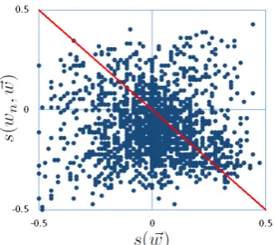
[image:1.595.334.486.208.343.2]Morante and Sporleder (2012) define negation to be “a grammatical category that allows the chang-ing of the truth value of a proposition”. Nega-tion is often expressed through the use of nega-tive signals or negators–words like isn’t and never, and it can significantly affect the sentiment of its scope. Understanding the impact of negation on sentiment is essential in automatic analysis of sentiment. The literature contains interesting re-search attempting to model and understand the behavior (reviewed in Section 2). For example,
Figure 1: Effect of a list of common negators in modifying sentiment values in Stanford Senti-ment Treebank. The x-axis is s(~w), and y-axis is s(wn, ~w). Each dot in the figure corresponds to a text span being modified by (composed with) a negator in the treebank. The red diagonal line corresponds to the sentiment-reversing hypothesis that simply reverses the sign of sentiment values.
a simple yet influential hypothesis posits that a negator reverses the sign of the sentiment value of the modified text (Polanyi and Zaenen, 2004; Kennedy and Inkpen, 2006). The shifting hypoth-esis (Taboada et al., 2011), however, assumes that negators change sentiment values by a constant amount. In this paper, we refer to a negation word as the negator (e.g., isn’t), a text span being mod-ified by and composed with a negator as the
ar-gument (e.g., very good), and entire phrase (e.g., isn’t very good) as the negated phrase.
The recently available Stanford Sentiment Tree-bank (Socher et al., 2013) renders manually anno-tated, real-valued sentiment scores for all phrases in parse trees. This corpus provides us with the data to further understand the quantitative behav-ior of negators, as the effect of negators can now be studied with arguments of rich syntactic and se-mantic variety. Figure 1 illustrates the effect of a common list of negators on sentiment as observed
on the Stanford Sentiment Treebank.1 Each dot in the figure corresponds to a negated phrase in the treebank. The x-axis is the sentiment score of its
argument s(~w) and y-axis the sentiment score of the entire negated phrases(wn, ~w).
We can see that the reversing assumption (the red diagonal line) does capture some regularity of human perception, but rather roughly. Moreover, the figure shows that same or similars(~w)scores (x-axis) can correspond to very differents(wn, ~w) scores (y-axis), which, to some degree, suggests the potentially complicated behavior of negators.2
This paper describes a quantitative study of the effect of a list of frequent negators on sen-timent. We regard the negators’ behavior as an underlying function embedded in annotated data; we aim to model this function from different as-pects. By examining sentiment compositions of negators and arguments, we model the quantita-tive behavior of negators in changing sentiment. That is, given a negated phrase (e.g., isn’t very
good) and the sentiment score of its argument
(e.g., s(“very good′′) = 0.5), we focus on un-derstanding the negator’s quantitative behavior in yielding the sentiment score of the negated phrase
s(“isn′t very good′′).
We first evaluate the modeling capabilities of two influential heuristics and show that they cap-ture only very limited regularity of negators’ ef-fect. We then extend the models to be dependent on the negators and demonstrate that such a sim-ple extension can significantly improve the per-formance of fitting to the human annotated data. Next, we evaluate a recently proposed composi-tion model (Socher, 2013) that relies on both the negator and the argument. This model learns the syntax and semantics of the negator’s argument with a recursive neural network. This approach performs significantly better than those mentioned above. In addition, we explicitly incorporate the prior sentiment of the argument and observe that this information helps reduce fitting errors.
1The sentiment values have been linearly rescaled from the original range [0, 1] to [-0.5, 0.5]; in the figure a negative or positive value corresponds to a negative or a positive sen-timent respectively; zero means neutral. The negator list will be discussed later in the paper.
2Similar distribution is observed in other data such as Tweets (Kiritchenko et al., 2014).
2 Related work
Automatic sentiment analysis The expression of
sentiment is an integral component of human lan-guage. In written text, sentiment is conveyed with word senses and their composition, and in speech also via prosody such as pitch (Mairesse et al., 2012). Early work on automatic sentiment anal-ysis includes the widely cited work of (Hatzivas-siloglou and McKeown, 1997; Pang et al., 2002; Turney, 2002), among others. Since then, there has been an explosion of research addressing various aspects of the problem, including detecting sub-jectivity, rating and classifying sentiment, label-ing sentiment-related semantic roles (e.g., target of sentiment), and visualizing sentiment (see sur-veys by Pang and Lee (2008) and Liu and Zhang (2012)).
Negation modeling Negation is a general
gram-matical category pertaining to the changing of the truth values of propositions; negation modeling is not limited to sentiment. For example, paraphrase and contradiction detection systems rely on detect-ing negated expressions and opposites (Harabagiu et al., 2006). In general, a negated expression and the opposite of the expression may or may not con-vey the same meaning. For example, not alive has the same meaning as dead, however, not tall does not always mean short. Some automatic methods to detect opposites were proposed by Hatzivas-siloglou and McKeown (1997) and Mohammad et al. (2013).
Negation modeling for sentiment An early yet
influential reversing assumption conjectures that a negator reverses the sign of the sentiment value of the modified text (Polanyi and Zaenen, 2004; Kennedy and Inkpen, 2006), e.g., from +0.5 to -0.5, or vice versa. A different hypothesis, called the shifting hypothesis in this paper, assumes that negators change the sentiment values by a con-stant amount (Taboada et al., 2011; Liu and Sen-eff, 2009). Other approaches to negation modeling have been discussed in (Jia et al., 2009; Wiegand et al., 2010; Lapponi et al., 2012; Benamara et al., 2012).
within a predefined range after a negator.
There exist different ways of incorporating more complicated syntactic and semantic infor-mation. Much recent work considers sentiment analysis from a semantic-composition perspec-tive (Moilanen and Pulman, 2007; Choi and Cardie, 2008; Socher et al., 2012; Socher et al., 2013), which achieved the state-of-the-art perfor-mance. Moilanen and Pulman (2007) used a col-lection of hand-written compositional rules to as-sign sentiment values to different granularities of text spans. Choi and Cardie (2008) proposed a learning-based framework. The more recent work of (Socher et al., 2012; Socher et al., 2013) pro-posed models based on recursive neural networks that do not rely on any heuristic rules. Such mod-els work in a bottom-up fashion over the parse tree of a sentence to infer the sentiment label of the sentence as a composition of the sentiment ex-pressed by its constituting parts. The approach leverages a principled method, the forward and backward propagation, to learn a vector represen-tation to optimize the system performance. In principle neural network is able to fit very compli-cated functions (Mitchell, 1997), and in this paper, we adapt the state-of-the-art approach described in (Socher et al., 2013) to help understand the behav-ior of negators specifically.
3 Negation models based on heuristics
We begin with previously proposed methods that leverage heuristics to model the behavior of nega-tors. We then propose to extend them to consider lexical information of the negators themselves.
3.1 Non-lexicalized assumptions and modeling
In previous research, some influential, widely adopted assumptions posit the effect of negators to be independent of both the specific negators and the semantics and syntax of the arguments. In this paper, we call a model based on such assumptions a non-lexicalized model. In general, we can sim-ply define this category of models in Equation 1. That is, the model parameters are only based on the sentiment value of the arguments.
s(wn, ~w)def= f(s(~w)) (1)
3.1.1 Reversing hypothesis
A typical model falling into this category is the
reversing hypothesis discussed in Section 2, where
a negator simply reverses the sentiment scores(~w) to be−s(~w); i.e.,f(s(~w)) =−s(~w).
3.1.2 Shifting hypothesis
Basic shifting Similarly, a shifting based model
depends ons(~w)only, which can be written as:
f(s(~w)) =s(~w)−sign(s(~w))∗C (2)
where sign(.) is the standard sign function which determines if the constant C should be added to or deducted from s(wn): the constant is added to a negatives(~w)but deducted from a pos-itive one.
Polarity-based shifting As will be shown in our
experiments, negators can have different shifting power when modifying a positive or a negative phrase. Thus, we explore the use of two different constants for these two situations, i.e.,f(s(~w)) = s(~w)−sign(s(~w))∗C(sign(s(~w))). The constant C now can take one of two possible values. We will show that this simple modification improves the fitting performance statistically significantly. Note also that instead of determining these con-stants by human intuition, we use the training data to find the constants in all shifting-based models as well as for the parameters in other models.
3.2 Simple lexicalized assumptions
The above negation hypotheses rely on s(~w). As intuitively shown in Figure 1, the capability of the non-lexicalized heuristics might be limited. Fur-ther semantic or syntactic information from eiFur-ther the negators or the phrases they modify could be helpful. The most straightforward way of expand-ing the non-lexicalized heuristics is probably to make the models to be dependent on the negators.
s(wn, ~w)def= f(wn, s(~w)) (3)
Negator-based shifting We can simply extend the
basic shifting model above to consider the lexi-cal information of negators: f(s(~w)) = s(~w)− sign(s(~w))∗C(wn). That is, each negator has its own C. We call this model negator-based
shift-ing. We will show that this model also statistically
Combined shifting We further combine the
negator-based shifting and polarity-based shift-ing above: f(s(~w)) = s(~w) − sign(s(~w)) ∗
C(wn, sign(s(~w))). This shifting model is
based on negators and the polarity of the text they modify: constants can be different for each negator-polarity pair. The number of parameters in this model is the multiplication of number of negators by two (the number of sentiment polarities). This model further improves the fitting performance on the test data.
4 Semantics-enriched modeling
Negators can interact with arguments in complex ways. Figure 1 shows the distribution of the ef-fect of negators on sentiment without considering further semantics of the arguments. The question then is that whether and how much incorporating further syntax and semantic information can help better fit or predict the negation effect. Above, we have considered the semantics of the negators. Be-low, we further make the models to be dependent on the arguments. This can be written as:
s(wn, ~w)def= f(wn, s(~w), r(~w)) (4)
In the formula,r(~w)is a certain type of repre-sentation for the argument ~wand it models the se-mantics or/and syntax of the argument. There ex-ist different ways of implementingr(~w). We con-sider two models in this study: one dropss(~w)in Equation 4 and directly modelsf(wn, r(~w)). That is, the non-uniform information shown in Figure 1 is not directly modeled. The other takes into ac-counts(~w)too.
For the former, we adopt the recursive neu-ral tensor network (RNTN) proposed recently by Socher et al. (2013), which has showed to achieve the state-of-the-art performance in sentiment anal-ysis. For the latter, we propose a prior sentiment-enriched tensor network (PSTN) to take into ac-count the prior sentiment of the arguments(~w).
4.1 RNTN: Recursive neural tensor network
A recursive neural tensor network (RNTN) is a specific form of feed-forward neural network based on syntactic (phrasal-structure) parse tree to conduct compositional sentiment analysis. For completeness, we briefly review it here. More de-tails can be found in (Socher et al., 2013).
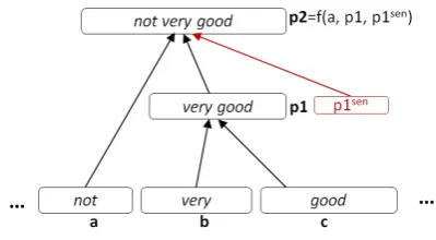
[image:4.595.317.517.64.174.2]As shown in the black portion of Figure 2, each instance of RNTN corresponds to a binary parse
Figure 2: Prior sentiment-enriched tensor network (PSTN) model for sentiment analysis.
tree of a given sentence. Each node of the parse tree is a fixed-length vector that encodes composi-tional semantics and syntax, which can be used to predict the sentiment of this node. The vector of a node, sayp2 in Figure 2, is computed from thed -dimensional vectors of its two children, namelya andp1(a, p1 ∈Rd×1), with a non-linear function:
p2 =tanh(
a
p1
T
V[1:d]a
p1
+W
a
p1
) (5)
where, W ∈ Rd×(d+d) andV ∈ R(d+d)×(d+d)×d are the matrix and tensor for the composition func-tion. A major difference of RNTN from the con-ventional recursive neural network (RRN) (Socher et al., 2012) is the use of the tensor V in order to directly capture the multiplicative interaction of two input vectors, although the matrix W implic-itly captures the nonlinear interaction between the
input vectors. The training of RNTN uses conven-tional forward-backward propagation.
4.2 PSTN: Prior sentiment-enriched tensor network
The non-uniform distribution in Figure 1 has showed certain correlations between the sentiment values of s(wn, ~w) and s(~w), and such informa-tion has been leveraged in the models discussed in Section 3. We intend to devise a model that imple-ments Equation 4. It bridges between the models we have discussed above that use either s(~w) or
r(~w).
p1, noted aspsen1 . As a result, the vector ofp2 is
calculated as follows:
p2 =tanh(
a
p1
T
V[1:d]
a
p1
+W
a
p1
(6)
+
a
psen
1
T
Vsen[1:d]
a
psen
1
+Wsen
a
psen
1
)
As shown in Equation 6, for the node vector p1 ∈Rd×1, we employ a matrix, namelyWsen ∈
Rd×(d+m)and a tensor,Vsen∈R(d+m)×(d+m)×d, aiming at explicitly capturing the interplays be-tween the sentiment class ofp1, denoted aspsen1 (∈
Rm×1), and the negator a. Here, we assume the
sentiment task hasmclasses. Following the idea of Wilson et al. (2005), we regard the sentiment of p1 as a prior sentiment as it has not been affected
by the specific context (negators), so we denote our method as prior sentiment-enriched tensor net-work (PSTN). In Figure 2, the red portion shows the added components of PSTN.
Note that depending on different purposes,psen1 can take the value of the automatically predicted sentiment distribution obtained in forward propa-gation, the gold sentiment annotation of nodep1, or even other normalized prior sentiment value or confidence score from external sources (e.g., sen-timent lexicons or external training data). This is actually an interesting place to extend the cur-rent recursive neural network to consider extrinsic knowledge. However, in our current study, we fo-cus on exploring the behavior of negators. As we have discussed above, we will use the human an-notated sentiment for the arguments, same as in the models discussed in Section 3.
With the new matrix and tensor, we then have
θ = (V, Vsen, W, Wsen, Wlabel, L) as the PSTN
model’s parameters. Here, L denotes the vector representations of the word dictionary.
4.2.1 Inference and Learning
Inference and learning in PSTN follow a forward-backward propagation process similar to that in (Socher et al., 2013), and for completeness, we depict the details as follows. To train the model, one first needs to calculate the predicted sentiment distribution for each node:
psen
i =Wlabelpi, pseni ∈Rm×1
and then compute the posterior probability over themlabels:
yi=softmax(pseni )
During learning, following the method used by the RNTN model in (Socher et al., 2013), PSTN also aims to minimize the cross-entropy error be-tween the predicted distribution yi ∈ Rm×1 at nodeiand the target distributionti ∈Rm×1at that node. That is, the error for a sentence is calculated as:
E(θ) =X
i X
j
tijlogyij+λkθk2 (7)
where, λ represents the regularization hyperpa-rameters, and j ∈ m denotes thej-th element of the multinomial target distribution.
To minimize E(θ), the gradient of the objec-tive function with respect to each of the param-eters in θ is calculated efficiently via backprop-agation through structure, as proposed by Goller and Kchler (1996). Specifically, we first compute the prediction errors in all tree nodes bottom-up. After this forward process, we then calculate the derivatives of the softmax classifiers at each node in the tree in a top-down fashion. We will discuss the gradient computation for the Vsenand Wsen in detail next. Note that the gradient calculations for theV, W, Wlabel, Lare the same as that of pre-sented in (Socher et al., 2013).
In the backpropogation process of the training, each node (except the root node) in the tree car-ries two kinds of errors: the local softmax error and the error passing down from its parent node. During the derivative computation, the two errors will be summed up as the complement incoming error for the node. We denote the complete incom-ing error and the softmax error vector for node i
asδi,com ∈ Rd×1 and δi,s ∈ Rd×1, respectively.
With this notation, the error for the root node p2 can be formulated as follows.
δp2,com=δp2,s
= (WT(yp2 −tp2))⊗f′([a;p
1]) (8)
where⊗is the Hadamard product between the two vectors and f′ is the element-wise derivative of f = tanh. With the results from Equation 8, we then can calculate the derivatives for theWsenat nodep2using the following equation:
∂Ep2
Wsen =δp2,com([a;psen1 ])T
1, . . . , d) of theVsentensor, we have the follow-ing:
∂Ep2
Vsen
[k]
=δp2,com k
a
psen
1
a
psen
1
T
Now, let’s form the equations for computing the error for the two children of thep2 node. The dif-ference for the error at p2 and its two children is that the error for the latter will need to compute the error message passing down from p2. We denote the error passing down asδp2,down, where the left child and the right child ofp2take the 1stand 2nd half of the error δp2,down, namelyδp2,down[1 : d]
and δp2,down[d+ 1 : 2d], respectively.
Follow-ing this notation, we have the error message for the two children ofp2, provided that we have the
δp2,down:
δp1,com=δp1,s+δp2,down[d+ 1 : 2d]
= (WT(yp1 −tp1))⊗f′([b;c])
+δp2,down[d+ 1 : 2d]
The incoming error message of node acan be calculated similarly. Finally, we can finish the above equations with the following formula for computingδp2,down:
δp2,down = (WTδp2,com)⊗f′([a;p1]) +δtensor
where
δtensor= [δV[1 :d] +δVsen
[1 :d], δV[d+ 1 : 2d]]
=
d
X
k=1
δp2,com
k (V[k]+ (V[k])T)⊗f
′
([a;p1])[1 :d]
+Xd
k=1
δp2,com
k (V[senk] + (V[senk] )T)⊗f
′ ([a;psen
1 ])[1 :d]
+Xd
k=1
δp2,com
k (V[k]+ (V[k])T)⊗f
′
([a;p1])[d+ 1 : 2d]
After the models are trained, they are applied to predict the sentiment of the test data. The orig-inal RNTN and the PSTN predict 5-class senti-ment for each negated phrase; we map the out-put to real-valued scores based on the scale that Socher et al. (2013) used to map real-valued senti-ment scores to sentisenti-ment categories. Specifically, we conduct the mapping with the formula: preali = yi·[0.1 0.3 0.5 0.7 0.9]; i.e., we calculate the dot product of the posterior probabilityyiand the scal-ing vector. For example, if yi = [0.5 0.5 0 0 0],
meaning this phrase has a 0.5 probability to be in the first category (strong negative) and 0.5 for the second category (weak negative), the resulting
preal
i will be 0.2 (0.5*0.1+0.5*0.3).
5 Experiment set-up
Data As described earlier, the Stanford Sentiment
Treebank (Socher et al., 2013) has manually anno-tated, real-valued sentiment values for all phrases in parse trees. This provides us with the training and evaluation data to study the effect of negators with syntax and semantics of different complex-ity in a natural setting. The data contain around 11,800 sentences from movie reviews that were originally collected by Pang and Lee (2005). The sentences were parsed with the Stanford parser (Klein and Manning, 2003). The phrases at all tree nodes were manually annotated with one of 25 sentiment values that uniformly span between the positive and negative poles. The values are nor-malized to the range of [0, 1].
In this paper, we use a list of most frequent negators that include the words not, no, never, and their combinations with auxiliaries (e.g., didn’t). We search these negators in the Stanford Senti-ment Treebank and normalize the same negators to a single form; e.g., “is n’t”, “isn’t”, and “is not” are all normalized to “is not”. Each occurrence of a negator and the phrase it is directly composed with in the treebank, i.e., hwn, ~wi, is considered a data point in our study. In total, we collected 2,261 pairs, including 1,845 training and 416 test cases. The split of training and test data is same as specified in (Socher et al., 2013).
Evaluation metrics We use the mean absolute
er-ror (MAE) to evaluate the models, which mea-sures the averaged absolute offsets between the predicted sentiment values and the gold stan-dard. More specifically, MAE is calculated as:
MAE = 1
N P
hwn, ~wi|(ˆs(wn, ~w)−s(wn, ~w))|,
wheresˆ(wn, ~w)denotes the gold sentiment value and s(wn, ~w) the predicted one for the pair
hwn, ~wi, and N is the total number of test in-stances. Note that mean square error (MSE) is an-other widely used measure for regression, but it is less intuitive for out task here.
6 Experimental results
Overall regression performance Table 1 shows
simply guesses the sentiment value for each test case randomly in the range [0,1]. The table shows that the basic reversing and shifting heuristics do capture negators’ behavior to some degree, as their MAE scores are higher than that of the baseline. Making the basic shifting model to be dependent on the negators (model 4) reduces the prediction error significantly as compared with the error of the basic shifting (model 3). The same is true for the polarity-based shifting (model 5), reflect-ing that the roles of negators are different when modifying positive and negative phrases. Merging these two models yields additional improvement (model 6).
Assumptions MAE
Baseline
(1) Random 0.2796
Non-lexicalized
(2) Reversing 0.1480*
(3) Basic shifting 0.1452* Simple-lexicalized
(4) Negator-based shifting 0.1415† (5) Polarity-based shifting 0.1417† (6) Combined shifting 0.1387† Semantics-enriched
(7) RNTN 0.1097**
(8) PSTN 0.1062††
Table 1: Mean absolute errors (MAE) of fitting different models to Stanford Sentiment Treebank. Models marked with an asterisk (*) are statisti-cally significantly better than the random baseline. Models with a dagger sign (†) significantly outper-form model (3). Double asterisks ** indicates a statistically significantly different from model (6), and the model with the double dagger††is signif-icantly better than model (7). One-tailed paired t-test with a 95% significance level is used here.
Furthermore, modeling the syntax and seman-tics with the state-of-the-art recursive neural net-work (model 7 and 8) can dramatically improve the performance over model 6. The PSTN model, which takes into account the human-annotated
prior sentiment of arguments, performs the best.
This could suggest that additional external knowl-edge, e.g., that from human-built resources or au-tomatically learned from other data (e.g., as in (Kiritchenko et al., 2014)), including sentiment that cannot be inferred from its constituent expres-sions, might be incorporated to benefit the current
is_ne
v
er
will_not is_not
does_not
barely
w
as_not
could_not
not
did_not unlik
ely
do_not
can_not
no
has_not
superficial would_not should_not
[image:7.595.315.524.85.226.2]0.05 0.10 0.15 0.20 0.25 0.30
Figure 3: Effect of different negators in shifting sentiment values.
neural-network-based models as prior knowledge. Note that the two neural network based models incorporate the syntax and semantics by represent-ing each node with a vector. One may consider that a straightforward way of considering the se-mantics of the modified phrases is simply memo-rizing them. For example, if a phrase very good modified by a negator not appears in the train-ing and test data, the system can simply memorize the sentiment score of not very good in training and use this score at testing. When incorporating this memorizing strategy into model (6), we ob-served a MAE score of 0.1222. It’s not surprising that memorizing the phrases has some benefit, but such matching relies on the exact reoccurrences of phrases. Note that this is a special case of what the neural network based models can model.
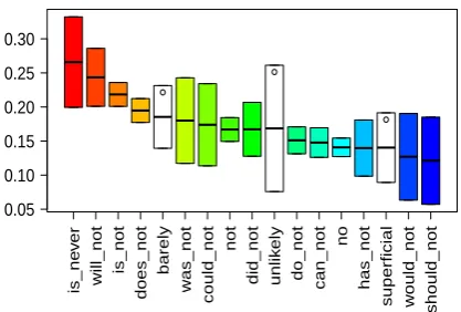
Discriminating negators The results in Table 1
[image:7.595.79.286.264.442.2]has demonstrated the benefit of discriminating negators. To understand this further, we plot in Figure 3 the behavior of different negators: the x-axis is a subset of our negators and the y-axis denotes absolute shifting in sentiment values. For example, we can see that the negator “is never” on average shifts the sentiment of the arguments by 0.26, which is a significant change considering the range of sentiment value is [0, 1]. For each negator, a 95% confidence interval is shown by the boxes in the figure, which is calculated with the bootstrapping resampling method. We can ob-serve statistically significant differences of shift-ing abilities between many negator pairs such as that between “is never” and “do not” as well as between “does not” and “can not”.
is_not(nn) is_not(np)
does_not(nn) does_not(np)
not(nn) not(np)
do_not(nn) do_not(np)
no(nn) no(np) 0.15
[image:8.595.308.531.63.230.2]0.20 0.25 0.30
Figure 4: The behavior of individual negators in negated negative (nn) and negated positive (np) context.
white bars), i.e., barely, unlikely, and superficial. By following (Kennedy and Inkpen, 2006), we ex-tracted 319 diminishers (also called
understate-ment or downtoners) from General Inquirer3. We calculated their shifting power in the same man-ner as for the negators and found three diminish-ers having shifting capability in the shifting range of these negators. This shows that the boundary between negators and diminishers can by fuzzy. In general, we argue that one should always con-sider modeling negators individually in a senti-ment analysis system. Alternatively, if the model-ing has to be done in groups, one should consider clustering valence shifters by their shifting abili-ties in training or external data.
Figure 4 shows the shifting capacity of negators when they modify positive (blue boxes) or nega-tive phrases (red boxes). The figure includes five most frequently used negators found in the sen-timent treebank. Four of them have significantly different shifting power when composed with pos-itive or negative phrases, which can explain why the polarity-based shifting model achieves im-provement over the basic shifting model.
Modeling syntax and semantics We have seen
above that modeling syntax and semantics through the-state-of-the-art neural networks help improve the fitting performance. Below, we take a closer look at the fitting errors made at different depths of the sentiment treebank. The depth here is de-fined as the longest distance between the root of a negator-phrase pair hwn, ~wi and their descendant
3
http://www.wjh.harvard.edu/ inquirer/
Figure 5: Errors made at different depths in the sentiment tree bank.
leafs. Negators appearing at deeper levels of the tree tend to have more complicated syntax and se-mantics. In Figure 5, the x-axis corresponds to different depths and y-axis is the mean absolute errors (MAE).
The figure shows that both RNTN and PSTN perform much better at all depths than the model 6 in Table 1. When the depths are within 4, the RNTN performs very well and the (human annotated) prior sentiment of arguments used in PSTN does not bring additional improvement over RNTN. PSTN outperforms RNTN at greater depths, where the syntax and semantics are more complicated and harder to model. The errors made by model 6 is bumpy, as the model considers no semantics and hence its errors are not depen-dent on the depths. On the other hand, the er-rors of RNTN and PSTN monotonically increase with depths, indicating the increase in the task dif-ficulty.
7 Conclusions
[image:8.595.87.283.90.230.2]per-formance statistically significantly. The detailed analysis reveals the differences in the behavior among negators, and we argue that they should al-ways be modeled separately. We further make the models to be dependent on the text being modi-fied by negators, through adaptation of a state-of-the-art recursive neural network to incorporate the syntax and semantics of the arguments; we dis-cover this further reduces fitting errors.
References
Farah Benamara, Baptiste Chardon, Yannick Mathieu, Vladimir Popescu, and Nicholas Asher. 2012. How do negation and modality impact on opinions? In
Proceedings of the ACL-2012 Workshop on Extra-Propositional Aspects of Meaning in Computational Linguistics, pages 10–18, Jeju, Republic of Korea.
Yejin Choi and Claire Cardie. 2008. Learning with compositional semantics as structural inference for subsentential sentiment analysis. In Proceedings of
the Conference on Empirical Methods in Natural Language Processing, EMNLP ’08, pages 793–801,
Honolulu, Hawaii.
Christoph Goller and Andreas Kchler. 1996. Learn-ing task-dependent distributed representations by backpropagation through structure. In In Proc. of
the ICNN-96, pages 347–352, Bochum, Germany.
IEEE.
Sanda Harabagiu, Andrew Hickl, and Finley Lacatusu. 2006. Negation, contrast and contradiction in text processing. In AAAI, volume 6, pages 755–762.
Vasileios Hatzivassiloglou and Kathleen R. McKeown. 1997. Predicting the semantic orientation of adjec-tives. In Proceedings of the 8th Conference of
Euro-pean Chapter of the Association for Computational Linguistics, EACL ’97, pages 174–181, Madrid,
Spain.
Lifeng Jia, Clement Yu, and Weiyi Meng. 2009. The effect of negation on sentiment analysis and retrieval effectiveness. In Proceedings of the 18th ACM
Con-ference on Information and Knowledge Manage-ment, CIKM ’09, pages 1827–1830, Hong Kong,
China. ACM.
Alistair Kennedy and Diana Inkpen. 2006.
Senti-ment classification of movie reviews using contex-tual valence shifters. Computational Intelligence, 22(2):110–125.
Svetlana Kiritchenko, Xiaodan Zhu, and Saif Moham-mad. 2014. Sentiment analysis of short informal texts. (to appear) Journal of Artificial Intelligence
Research.
Dan Klein and Christopher D. Manning. 2003. Ac-curate unlexicalized parsing. In Proceedings of the
41st Annual Meeting on Association for Computa-tional Linguistics - Volume 1, ACL ’03, pages 423–
430, Sapporo, Japan. Association for Computational Linguistics.
Emanuele Lapponi, Jonathon Read, and Lilja
Ovre-lid. 2012. Representing and resolving negation
for sentiment analysis. In Jilles Vreeken, Charles Ling, Mohammed Javeed Zaki, Arno Siebes, Jef-frey Xu Yu, Bart Goethals, GeofJef-frey I. Webb, and Xindong Wu, editors, ICDM Workshops, pages 687– 692. IEEE Computer Society.
Jingjing Liu and Stephanie Seneff. 2009. Review sen-timent scoring via a parse-and-paraphrase paradigm. In EMNLP, pages 161–169, Singapore.
Bing Liu and Lei Zhang. 2012. A survey of opin-ion mining and sentiment analysis. In Charu C. Ag-garwal and ChengXiang Zhai, editors, Mining Text
Data, pages 415–463. Springer US.
Franc¸ois Mairesse, Joseph Polifroni, and Giuseppe Di Fabbrizio. 2012. Can prosody inform sentiment analysis? experiments on short spoken reviews. In
ICASSP, pages 5093–5096, Kyoto, Japan.
Tom M Mitchell. 1997. Machine learning. 1997. Burr
Ridge, IL: McGraw Hill, 45.
Saif M. Mohammad, Bonnie J. Dorr, Graeme Hirst, and Peter D. Turney. 2013. Computing lexical contrast.
Computational Linguistics, 39(3):555–590.
Karo Moilanen and Stephen Pulman. 2007. Senti-ment composition. In Proceedings of RANLP 2007, Borovets, Bulgaria.
Roser Morante and Caroline Sporleder. 2012. Modal-ity and negation: An introduction to the special is-sue. Computational linguistics, 38(2):223–260.
Bo Pang and Lillian Lee. 2005. Seeing stars: Ex-ploiting class relationships for sentiment categoriza-tion with respect to rating scales. In Proceedings of
the Annual Meeting of the Association for Computa-tional Linguistics, ACL ’05, pages 115–124.
Bo Pang and Lillian Lee. 2008. Opinion mining and sentiment analysis. Foundations and Trends in
In-formation Retrieval, 2(1–2):1–135.
Bo Pang, Lillian Lee, and Shivakumar Vaithyanathan.
2002. Thumbs up? sentiment classification
us-ing machine learnus-ing techniques. In Proceedus-ings of
EMNLP, pages 79–86, Philadelphia, USA.
Livia Polanyi and Annie Zaenen. 2004. Contextual valence shifters. In Exploring Attitude and Affect in
Text: Theories and Applications (AAAI Spring Sym-posium Series).
Proceedings of the Conference on Empirical Meth-ods in Natural Language Processing, EMNLP ’12,
Jeju, Korea. Association for Computational Linguis-tics.
Richard Socher, Alex Perelygin, Jean Y. Wu, Jason Chuang, Christopher D. Manning, Andrew Y. Ng, and Christopher Potts. 2013. Recursive deep mod-els for semantic compositionality over a sentiment treebank. In Proceedings of the Conference on
Em-pirical Methods in Natural Language Processing,
EMNLP ’13, Seattle, USA. Association for Compu-tational Linguistics.
Maite Taboada, Julian Brooke, Milan Tofiloski,
Kim-berly Voll, and Manfred Stede. 2011.
Lexicon-based methods for sentiment analysis.
Computa-tional Linguistics, 37(2):267–307.
Peter Turney. 2002. Thumbs up or thumbs down? se-mantic orientation applied to unsupervised classifi-cation of reviews. In ACL, pages 417–424, Philadel-phia, USA.
Michael Wiegand, Alexandra Balahur, Benjamin Roth, Dietrich Klakow, and Andr´es Montoyo. 2010. A survey on the role of negation in sentiment analysis. In Proceedings of the Workshop on Negation and
Speculation in Natural Language Processing,
NeSp-NLP ’10, pages 60–68, Stroudsburg, PA, USA. As-sociation for Computational Linguistics.
Theresa Wilson, Janyce Wiebe, and Paul Hoffmann. 2005. Recognizing contextual polarity in phrase-level sentiment analysis. In Proceedings of the
Con-ference on Human Language Technology and Em-pirical Methods in Natural Language Processing,