Designing International Environmental Agreements under Participation Uncertainty

Munich Personal RePEc Archive

Designing International Environmental

Agreements under Participation

Uncertainty

Mao, Liang

College of Economics, Shenzhen University

15 May 2017

Online at

https://mpra.ub.uni-muenchen.de/79145/

Designing International Environmental

Agreements under Participation Uncertainty

Liang Mao

May 2017

Abstract

We analyze the design of optimal international environmental a-greement (IEA) by a three-stage coalition formation game. A certain degree of participation uncertainty exists in that each country choos-ing to sign the IEA for its best interest has a probability to make a mistake and end up a non-signatory. The IEA rule, which specifies the action of each signatory for each coalition formed, is endogenously de-termined by a designer, whose goal is to maximize the expected payoff of each signatory. We provide an algorithm to determine an optimal rule and compare this rule to some popular rules used in the literature.

Keywords: International environmental agreement, coalition forma-tion, participation uncertainty, stable coalition

JEL codes: Q54, C72, H41

∗_{College of Economics, Shenzhen University, Shenzhen, Guangdong, 518060, China.}

1

Introduction

The human society is facing a serious threat of climate change, mainly due to the emission of greenhouse gases (GHG). For a country, reducing the e-mission of GHG can be regarded as providing a public good benefiting the whole world. However, voluntary abatement of GHG is typically not suffi-cient, because every country has an incentive to free ride on the abatement effort of other countries. One method to overcome this free-riding problem is to form a coalition wherein the members sign a self-enforcing internation-al environmentinternation-al agreement (IEA) and follow certain abatement rules. The Kyoto Protocol and the Paris Agreement are examples of such IEAs.

The formation of these coalitions is sometimes modeled as a two-stage game, or its variant, played by some self-interested countries.1 _{In stage one}

(participation stage), each country decides whether to join the coalition and sign the IEA. In stage two (abatement stage), those signing the IEA have to follow the IEA rule, while each non-signatory can decide its own abatement level.

Nevertheless, it is reported that IEAs do not work very well. For instance, Kellenberg and Levinson (2014) suggest that “IEAs appear to do little more than ratify what countries would have done absent the agreements.” There could be many reasons for the failure of IEAs, but in this paper, we focus only on the following two of them.

First, the IEA rule is typically exogenously given and may not provide for much incentive to overcome the free-riding problem. For instance, a large body of studies assume that in stage two of the game, all coalition members should coordinate their actions and maximize the total payoffs of the coalition formed in stage one. We call this IEA rule the maximal total payoff (MTP) rule. In section 5, we will show that the MTP rule is generally not optimal. In order to overcome the problem raised by exogenous IEA rules, several studies analyzed the endogenous determination of the IEA rules. For exam-ple, Carraro et al. (2009) discuss the MTP rule with an additional restriction

1

of minimal participation; here, the threshold of forming the coalition is en-dogenously determined. K¨oke and Lange (2017) considers an endogenous rule that simultaneously determine the threshold of cooperation and the sig-natories’ abatement level. However, these studies analyze only certain special cases of endogenous rules and hence cannot be considered fully general. In particular, a signatory’s abatement level as specified by these rules need not vary endogenously according to the coalition formed in stage one, except when the change involves the minimal participation condition.

The second reason for the IEAs’ failure is participation uncertainty: a country initially intending to sign the IEA for its own interest has a chance to make a mistake and end up a non-signatory. This uncertainty, which makes it more difficult to form a large coalition, may be due to various reasons under different cases. For example, ratification of the IEA may be prevented by some interest groups2_{, or a newly elected leader may overturn the decision}

made by his predecessor. In contrast, we assume that the probability that a country not intending to sign the IEA becomes a signatory, which rarely happens in reality, is zero. Also note that participation uncertainty is unlike several other types of risk and uncertainty discussed in the IEA literature.3

The main purpose of this study is to extend the traditional coalition formation models of IEA to allow for participation uncertainty and fully general rules that are endogenously determined. We hope these extensions will help us design a better IEA rule than the ones used in reality and those in the literature. To this end, we employ a three-stage coalition formation game. In stage one (designing stage), a designer4 _{launches an coalition and}

announces an IEA rule, which is a function specifies the abatement level of a signatory (coalition member) for each possible coalition formed in stage two of the game. As the initiator of the coalition, the designer’s goal is to maximize the expected payoff of each signatory. Stage two extends the usual participation stage by assuming a given probability ε ≥0 that each country choosing to sign the IEA would finally end up not being a coalition member.

2

See K¨oke and Lange (2017).

3

See, among others, Kolstad (2007), Dellink et al. (2008), Kuiper and Olaizola (2008), Hong and Karp (2014), Cazals and Sauquet (2015), and Masoudi et al. (2016).

4

Stage three is the usual abatement stage that determines each country’s abatement level and payoff.

This three-stage game can be solved by backward induction. Thus, we determine the optimal rule that the designer would announce in stage one and the coalition of countries that intend to sign the IEA in stage two. Note that participation uncertainty would make it more difficult to determine the coalition that will form in stage two. Given the IEA rule announced in stage one, a coalition will be formed if and only if it is stable; that is, no country would change its participation decision both before and after observing the mistakes made by some other countries. We prove that given any IEA rule, the cardinality of a stable coalition can be uniquely determined (Proposition 1). Furthermore, we provide an algorithm to determine an optimal rule for the designer (Theorem 1).

Some IEA rules, for example, the MTP rule, the minimal participation rule, and the coalition unanimity rule, are commonly used in the literature. We show through an example that these rules are generally not optimal for the designer. Additionally, we briefly discuss the conditions under which these rules are optimal (Proposition 2, 3).

The remainder of this paper is organized as follows. Section 2 presents the setup of the model and the three-stage coalition formation game. We solve this game and derive an optimal IEA rule in section 3 and 4. Some traditional IEA rules are discussed and compared with the optimal rule in section 5. Finally, section 6 concludes the paper.

2

The model

Let N = {1,2, . . . , n} be a set of homogeneous countries, where n ≥ 2. There is a perfectly divisible good with negative externalities, for example, greenhouse gas. Furthermore, let xi denote country i’s abatement level of

Given x, country i’s payoff is

ui(x) = α

X

j∈N

xj −

1 2x

2

i, (1)

where α >0 is the constant marginal benefit from total abatementP

j∈N xj

due to negative externalities of the good, and x2

i/2 is country i’s abatement

cost. Assume that payoffs are transferable, and therefore social welfare is the total payoffs of all countries:

U(x) =X

i∈N

ui(x) =nα

X

i∈N

xi−

X

i∈N

x2 i

2 .

An abatement combination (x∗

1, . . . , x∗n) is said to be socially optimal if it

maximizes social welfare. The first-order conditions ∂U(x)/∂xi = 0 yield

x∗

i =nα, ∀i∈N. (2)

On the other hand, if each countryi choosesxi to maximize its own

pay-off ui given the other countries’ abatement levels, the first-order conditions

∂ui(x)/∂xi = 0 lead to

¯

xi =α, ∀i∈N. (3)

Note that ¯xi is a dominant abatement level of i, regardless of other

coun-tries’ actions. From this, it follows that ¯x= (¯x1, . . . ,x¯n) is the unique Nash

equilibrium of this non-cooperative abatement game. Since x∗

i > x¯i, the world suffers from too much emission of the good.

This is a commonly known social dilemma due to externalities. One possible method to partially overcome this problem is to form a coalition that reg-ulates the countries’ actions by a self-enforcing IEA. The formation of the coalition follows a three-stage game.

• Stage one. A designer announces an IEA rule e, which is a function assigning a real value e(m) ≥0 to each integer m ∈ [1, n], where m is the cardinality of the coalition M that will be formed in stage two. A rule can be denoted by the vector e= e(1), . . . , e(n)

• Stage two. All countries in N simultaneously decide whether or not to sign the IEA. Let M denote the set of countries that choose to sign and m = |M| denote its cardinality. However, there is a one-way uncertainty with regard to each country’s final participation decision. Specifically, each countryi∈M has a probabilityεof making a mistake and failing to sign the IEA, where 0 ≤ ε < 1 is exogenously given. However, each j /∈M never makes a mistake and would certainly not sign the IEA. LetM denote the set of signatory countries that choose to sign the IEA and make no mistake, andm=|M|denote its cardinality. Given m and ε ∈ (0,1), m follows a binomial distribution so that the probability that m=k is

b(k;m,1−ε) = m!

k!(m−k)!ε

m−k_(1−ε)k_{, ∀k = 0,1, . . . , m.}

Additionally, if ε= 0, then b(m;m,1) = 1, b(k;m,1) = 0, ∀k < m.

• Stage three. Given rule e and the coalition M, each signatory i ∈ M

carries out its abatement xi = e(m) according to e, while each

non-signatory j /∈ M chooses its dominant abatement level xj = α. All

countries receive their respective payoffs according to (1).

Now, letG(n, α, ε) denote this three-stage game. Assume that each coun-try is risk neutral and chooses its action to maximize its expected payoff. We also assume that a country will choose to sign the IEA if it is indifferent be-tween signing and not signing. The designer will choose e∈_Rn

+ to maximize

the (identical) expected value of the payoff of each signatory i∈M.

3

Stable coalition and equilibrium scale

We solve game G(n, α, ε) by backward induction. Consider stage three first. Given e and m, let

denote the total abatement of all countries. Now, a signatory’s payoff is

uC_{(m, e) =αX(m, e)−} e(m)2

2 , if m≥1. (4)

Additionally, let

uC_{(0, e) =u}

i(¯x) = (n−1/2)α2. (5)

A non-signatory’s payoff is

uI(m, e) = αX(m, e)− α

2

2 , if m < n.

In stage two of G(n, α, ε), given e and m−i = |M\{i}|, country i’s

ex-pected payoff is

uC_(m

−i+ 1, e) = m−i

X

k=0

b(k;m−i,1−ε)

εuI_{(k, e) + (1−ε)u}C_{(k+ 1, e)}

if i chooses to sign the IEA (i∈M), and it is

uI_(m

−i, e) = m−i

X

k=0

b(k;m−i,1−ε)uI(k, e)

if i chooses not to sign (i /∈ M). In other words, uC_{(m, e) and u}I_{(m, e) are}

the expected payoffs of a country that chooses to sign and not to sign the IEA, respectively, when exactly m countries choose to sign the IEA.

We use the concept of stable coalition to predict which countries choose to sign the IEA in stage two. Roughly speaking, a coalition M is stable if the countries in the coalition are the only ones choosing to sign the IEA before any mistake occurs (ex ante stable), and countries that do not make mistakes will not change their decisions after some other countries have made mistakes (ex post stable).

Formally, following d’Aspremont et al. (1983) and many others, coalition

M is said to be ex ante stable relative to e if no country i ∈ M is willing to unilaterally leave M and no country j /∈M is willing to unilaterally join

stable relative to e if

uC(m, e)≥uI(m−1, e), uC(m+ 1, e)< uI(m, e).

In addition, M =∅ isex ante stable relative toe ifuC_{(1, e)< u}I_{(0, e), while}

M =N isex ante stable relative toe if uC_{(n, e)≥u}I_{(n−1, e).}

A coalitionM 6=∅is said to be ex post stable relative to eif no signatory will regret its decision to sign the IEA and withdraw after uncertainty is realized, no matter how many countries in M have made mistakes; that is,

uC(k+ 1, e)≥uI(k, e), ∀k∈[0, m−1].

In addition, M =∅ is trivially ex post stable relative to any e∈_Rn +.

Finally, M is said to be stable relative to e if it is both ex ante stable relative to e and ex post stable relative to e. Ultimately, a stable coalition will not provide any incentive for any country to change its decision regarding participation under any circumstance. Consequently,

(a) M =∅ is stable relative toe if

uC_{(1, e)< u}I_{(0, e); (6)}

(b) M /∈ {∅, N} is stable relative toe if

uC(m+ 1, e)< uI(m, e), uC(k+ 1, e)≥uI(k, e), ∀k ∈[0, m−1]; (7)

(c) M =N is stable relative to e if

uC_{(k+ 1, e)≥u}I_{(k, e), ∀k ∈[0, n−1]. (8)}

Because of the symmetry of countries, whether a coalition M is stable relative to rule e depends only on m = |M|. If a coalition M is stable relative to e, then we say that m is an equilibrium scale relative to e.

equilibrium scale relative toe. In other words, if the designer announces rule

ein stage one, then in stage two there will bem(e) countries choosing to sign the IEA. In the proof of this proposition, we provide an algorithm to derive

m(e) for each e∈_Rn +.

Proposition 1. There is a unique equilibrium scale relative to eache∈Rn +.

Proof. First, we prove that there exists at most one equilibrium scale relative to any e. Assume for a contradiction that both m1 and m2 are equilibrium

scales relative to some e, where m1 < m2. Since m1 is an equilibrium scale,

we have uC_(m

1 + 1, e) < uI(m1, e), which contradicts the assumption that

m2 is also an equilibrium scale.

If uC_{(1, e) < u}I_{(0, e), then m(e) = 0; otherwise, we have u}C_{(1, e) ≥}

uI_{(0, e). Furthermore, if u}C_{(2, e) < u}I_{(1, e), then m(e) = 1; otherwise, we}

have uC_{(1, e)≥ u}I_{(0, e), u}C_{(2, e) ≥ u}I_{(1, e). Proceeding in this manner, we}

shall either find an equilibrium scalem(e)< n, or eventually haveuC_{(k, e)≥}

uI_{(k−1, e),k = 1,2, . . . , n, which implies that m(e) =n.}

Givene∈Rn

+, letEuC(e) denote the expected payoff of a signatory. Since

there arem(e) countries intending to sign the IEA, the probability that there are exactly k signatories isb k;m(e),1−ε

for all k ≤m(e). Thus, we have

EuC(e) =

m(e)

X

k=0

b k;m(e),1−ε

uC(k, e). (9)

It follows from (5) that that when no country signs the IEA, the designer will take a non-signatory’s payoff as a substitute for a signatory’s payoff; we make this trivial assumption only to ensure that the objective of the designer is always well-defined.

4

An optimal rule

Now, consider stage one of G(n, α, ε). The objective of the designer in this stage is to maximize EuC_{(e) by choosing an appropriate rule e. If a rule e}

exists such that EuC_{(e) ≥ Eu}C_(e′_{) for all e}′ _∈

optimal. The following theorem shows that there always exists an optimal rule. The proof explicitly demonstrates how to construct an optimal rule.

Theorem 1. For any game G(n, α, ε), there exists an optimal rule e∗_.

Proof. For each integer s∈[0, n], let E(s) ={e∈Rn

+|m(e) =s} be the set

of rules whose equilibrium scale is s. Additionally, for each s∈[1, n], define

E(s) =

e(1), . . . , e(s)

∈Rs+|uC(k+1, e)≥uI(k, e), ∀k ∈[0, s−1] . (10)

Now, it is obvious that, ife= e(1), . . . , e(n)

∈E(s), then e(1), . . . , e(s)

∈

E(s). The proof of the following lemma is in the appendix.

Lemma 1. For each s∈[1, n], E(s) is a non-empty bounded closed set.

If m(e) = 0, then from (6), we have e(1) 6= α. Therefore, EuC_{(e) =}

(n−1₂)α2 _{for all e∈E(0) ={e∈R}n

+|e(1)6=α}.

Ifm(e) = 1, then from (7), we can easily obtainE(1) ={e∈_Rn

+|e(1) =

α, e(2) ∈(−∞, α)∪(3α,∞)}, EuC_{(e) = εu}C_{(0, e) + (1−ε)u}C_{(1, e) = (n−} 1

2)α2 for all e∈E(1).

If m(e) = 2, then again from (7), we have E(2) = {e ∈ _Rn

+|e(1) =

α, e(2)∈[α,3α], e(3)∈(−∞, f1(e(2)))∪(f2(e(2)),∞)}, wheref1 andf2 are

two functions that can be easily determined, but are irrelevant to our analysis. When e ∈ E(2), EuC_{(e) = ε}2_uC_{(0, e) + 2ε(1−ε)u}C_{(1, e) + (1−ε)}2_uC_{(2, e)}

depends only on e(1) and e(2). Therefore, we have maxe∈E(2)EuC(e) =

max_(e(1),e(2))∈E(2)EuC(e). Similarly, fors∈[2, n], we have

max

e∈E(s)Eu

C_{(e) = max}

(e(1),...,e(s))∈E(s)Eu C_(e).

Now, for any s ∈ [1, n], there exists e∗

s = e∗s(1), . . . , e∗s(n)

∈ E(s) such that EuC_(e∗

s) ≥ EuC(e′) for all e′ ∈ E(s). That is, EuC(e∗s) =

maxe∈E(s)EuC(e). In fact, from Lemma 1, we can derive e∗s(1), . . . , e ∗ s(s)

by solving the constrained optimization problem max_{(e(1),...,e(s))}∈E(s)EuC(e),5

and e∗

s(s+1), . . . , e ∗ s(n)

can be any vector as long asuC_{(s+1, e}∗

s)< uI(s, e ∗ s).

5

Finally, the maximal value ofEuC_{(e) equals max}

1≤s≤nmaxe∈E(s)EuC(e).

An optimal rule e∗

can thus be found, where

EuC(e∗

) = max

1≤s≤n{Eu C

(e∗

1), Eu C

(e∗

2), . . . , Eu C

(e∗ n)}.

This ends the proof of the proposition.

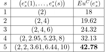
As an example, consider game G(5,2,0.1). In Table 1, we list for each

s ∈[1,5] the value of EuC_(e∗

s), which is the maximal value of EuC(e) under

the condition m(e) = s, as well as the corresponding rules e∗

s(1), . . . , e ∗ s(s)

. Since EuC_(e∗

5) > EuC(e∗4) > EuC(e∗3) > EuC(e∗2) > EuC(e∗1), we have e∗ =

e∗

5 = (2,2,3.61,6.44,10), and EuC(e∗) = 42.78.

Table 1: Calculating optimal rule e∗ _{for G(5,2,0.1)}

s e∗

s(1), . . . , e∗s(s)

EuC(e∗

s)

1 (2) 18

2 (2, 4) 19.62

3 (2, 4, 6) 24.32

4 (2, 2.95, 5.23, 8) 32.13 5 (2, 2, 3.61, 6.44, 10) 42.78

5

Discussion

Now, we discuss some special rules commonly used in the literature and compare them to the optimal rule e∗_.

(a) A rule ea _{is called the MTP rule if it always aims to maximize the}

total payoffs of all signatories. Because of the symmetry of players, we have m·uC_{(m, e}a_{) ≥ m·u}C_{(m, e}′_{), or u}C_{(m, e}a_{) ≥ u}C_{(m, e}′_{), for}

all m ∈ [1, n] and e′ _∈ Rn

+. That is, for all m ∈ [1, n], ea maximizes

uC_{(m, e), and thus e}a_{(m) = αm.}

(b) A ruleeb_{is called a minimal participation rule}6_{if there existsm}∗ _{∈[2, n]}

such that eb_{(m) = α when 1 ≤ m < m}∗_{, and e}b_{(m) = q > α when}

6

m ≥ m∗_{. In other words, this rule requires an abatement level q for}

signatories when at least m∗

countries sign the IEA. In particular, if

m∗ _{=n, e}b _{is called the coalition unanimity rule}7_.

(c) A rule ec _{is called an MTP rule with minimal participation}8 _{if there}

exists m∗ _{∈ [2, n] such that e}c_{(m) = α for all 1 ≤ m < m}∗_{, and}

ec_{(m) =αm for all m≥m}∗_{. Hence,e}c _{is a combination of e}a _{and e}b_.

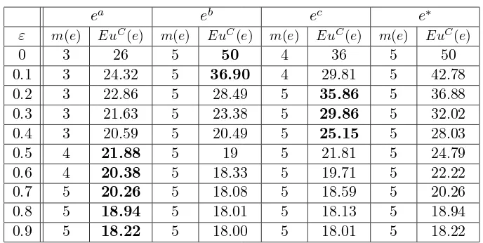
To compare these rules, we reconsider the example in the previous section where n = 5, α = 2. First, the MTP rule ea _{satisfies e}a_{(m) = 2m for all}

m ∈ [1, n]. Next, consider a coalition unanimity rule eb _{where e}b_{(m) = 2}

when m < 5 and eb_{(5) = 10. Finally, consider an MTP rule with minimal}

participation ec _{where e}c_{(4) = 8, e}c_{(5) = 10, and e}c_{(m) = 2 when m < 4.}

For these rules and the optimal rule e∗_{, we list the correspondingm(e) and}

EuC_{(e) for some particular value of ε in Table 2.}9 _{We shall explain and}

discuss the data in this table.

Table 2: Simulation for G(5,2, ε)

ea eb ec e∗

ε m(e) EuC_{(e) m(e) Eu}C_{(e) m(e) Eu}C_{(e) m(e) Eu}C_(e)

0 3 26 5 50 _{4 36 5 50}

0.1 3 24.32 5 36.90 _{4 29.81 5 42.78}

0.2 3 22.86 5 28.49 5 35.86 _{5 36.88}

0.3 3 21.63 5 23.38 5 29.86 _{5 32.02}

0.4 3 20.59 5 20.49 5 25.15 _{5 28.03}

0.5 4 21.88 _{5 19 5 21.81 5 24.79}

0.6 4 20.38 _{5 18.33 5 19.71 5 22.22}

0.7 5 20.26 _{5 18.08 5 18.59 5 20.26}

0.8 5 18.94 _{5 18.01 5 18.13 5 18.94}

0.9 5 18.22 _{5 18.00 5 18.01 5 18.22}

For the designer, a rule e has two important aspects that may affect the value of his objective EuC_{(e). On the one hand, the designer may wish}

7

See Chander and Tulkens (1997).

8

See Carraro et al. (2009).

9

more countries to sign the IEA and that the signatories engage in a high abatement level. Thus, the rule should provide for a strong incentive for cooperation or strong punishment for free riding by creating a large payoff gap between signing and not signing. On the other hand, the designer may also wish to reduce the harm that uncertainty brings on the expected payoffs of signatories. This can be accomplished only by designing a rule by which even when some countries do not sign the IEA due to mistakes, other signatories can still maintain a relatively high level of abatement, leading to a small payoff gap between signing and not signing.

We call these two aspects of the rules as incentive effect and uncertainty effect respectively. A rule has a strong/weak incentive effect if it provides strong/weak incentives for countries to sign the IEA; a rule has a strong/weak uncertainty effect if a certain ε has a small/large impact on EuC_(e).

The incentive effect and uncertainty effect are typically contradictory. For example, a rule with a strong uncertainty effect usually has a weak incentive effect. This is because any factor of the rule protecting the signatories from harm caused by uncertainty will require those signatories to maintain a high level of abatement regardless of the other countries’ mistakes. However, this requirement would also reduce the incentive for cooperation. An appropriate rule should have a good balance between the two conflicting effects.

From Table 2, of the three special rules we discussed above, the coalition unanimity rule eb _{is optimal when ε = 0. This is because e}b _{obviously has}

a strong incentive effect and weak uncertainty effect, but the latter is irrel-evant when ε = 0. Moreover, the next proposition shows that the coalition unanimity rule is almost optimal when uncertainty is sufficiently small.

Proposition 2. Supposeeb_{(n) =αn, ande}b_{(m) =α for all m < n. For any}

µ > 0, there exists γ >0 such that if ε < γ, EuC_(eb_{)> Eu}C_(e′_{)−µ, for all}

e′ _∈ Rn+.

Proof. It is obvious that m(eb_{) =n. Given any µ > 0, whenε is sufficiently}

small, EuC_(eb_{) =} Pn

k=0b k;n,1 −ε

uC_{(k, e}b_{) can be arbitrarily close to}

uC_{(n, e}b_{), and thus Eu}C_(eb_{) > u}C_{(n, e}b_{)−µ. From (4), it is easy to verify}

that uC_{(n, e}b_)≥uC_{(m, e}′_{) for all m ≤n and all e}′ _∈ Rn

uC_{(n, e}b_)−µ≥ Pm(e′)

k=0 b k;m(e

′_),1−ε

uC_{(k, e}′_)−µ=EuC_(e′_{)−µ, for all}

e′ _∈ Rn

+.

In contrast, from Table 2, the MTP ruleea _{is an optimal rule only when}

ε is large enough. This turns out to be a general outcome according to the next proposition, which suggests that the MTP rule has a relatively strong uncertainty effect.

Proposition 3. There exists θ >0 such that if ε > θ, ea _{is optimal.}

Proof. See the appendix.

Consider game G(5,2, ε) again and suppose that one country deviates from the grand coalition M =N because of a mistake. This deviation will cause each remaining signatory to reduce its abatement level by e(5)−e(4), which isea_(5)−ea_{(4) = 2 under the MTP rule, and ise}b_(5)−eb_{(4) = 8 under}

the coalition unanimity rule. This example illustrates why the MTP rule has a stronger uncertainty effect than the coalition unanimity rule.

The fact that the MTP rule may not be optimal under a small uncertainty seems to be counterintuitive at first glance. Once a coalition is formed, it is quite natural to require all signatories to act as one player and maximize their total payoffs. This explains why the MTP rule is so popular in the coalition formation literature. However, a shortcoming of the MTP rule is that it has a weak incentive effect and hence cannot effectively overcome the free-riding problem. Indeed, whenε is sufficiently small, the designer should require the maximization of total payoffs of coalition members for only a stable coalition, rather than for all coalitions. These redundant requirements lead to a weak incentive effect and undermine the MTP rule.

Finally, from Table 2, the MTP rule with minimal participation ec _can

be regarded as a mixture of ea _{and e}b_{. Hence, for the designer, e}c _{is better}

6

Concluding remarks

In this study, we introduce a three-stage coalition formation game to analyze the endogenous determination of the IEA rule under participation uncer-tainty. We provide an algorithm to derive an optimal rule, which reaches an appropriate balance between providing sufficient incentive for cooperation and reducing the losses caused by participation uncertainty.

We find that some commonly used rules are generally not optimal. In particular, the MTP rule has a weak incentive effect and is not optimal unless the uncertainty is very large; while the coalition unanimity rule has a weak uncertainty effect, it is optimal only when there is no participation uncertainty. Some of the failures of the IEAs in reality or in theory can be attributed to the inappropriate rules used under certain situations.

Some further works and extensions may be worth studying in future re-search. First, an open question is whether optimal rules are always (ex ante) efficient in the sense that they result in full participation and induce enough abatement level before uncertainty is realized; that is, m(e∗_{) = nand}

e∗_{(n) = nα. This question is important, because if the answer is positive,}

then we can be fairly optimistic about what IEAs may accomplish as long as their rules are properly designed. However, by now the author can neither prove the statement nor find an counterexample.

Second, we can study models with more general settings, for example, models with heterogeneous countries, or models with more general payoff function. Third, we may consider more complex IEA rules. For example, a rule may contain an emission function ei(M) specifying the abatement level

of i∈M and a transfer function ti(M) characterizing the amount of money

transferred to country i when coalition M is formed. Last but not least, some other goals of the designer can be studied. For instance, sometimes it makes more sense to assume that the designer will maximize expected social welfare rather than the signatories’ welfare.

R&D, and sharing natural resource.10 _{In a typical application, players first}

decide whether to join a coalition, and then all coalition members act ac-cording to the MTP rule. However, in most of these works, participation uncertainty is implicitly assumed to be zero, which implies that the MTP rule may not be an optimal rule for coalition members and the designer. Therefore, it is reasonable and necessary to re-examine the outcome of these works by endogenizing the choice of the coalition rules.

Appendix

Proof of Lemma 1.

(a) From (10), E(s) is obviously a closed set in _Rs

+ for each s∈[1, n].

(b) Now, we prove thatE(s) is a bounded set inRs

+by induction ons. We

can easily see that E(1) = {α} is bounded in R1+. Assume inductively that

E(k) is bounded inRk

+, 1≤k ≤n−1. That is, there existT1, T2, . . . , Tk >0,

such that for each e(1), . . . , e(k)

∈E(k): e(q)< Tq, 1 ≤q≤k.

Now, considerE(k+ 1). According to (10), for each e(1), . . . , e(k+ 1)

∈

E(k + 1), we have e(q) < Tq, 1 ≤ q ≤ k. Additionally, e(k+ 1) satisfies

uC_{(k+ 1, e)≥u}I_{(k, e); that is,}

−1

2e(k+ 1)

2_{+a(k+ 1)e(k+ 1) +A(k)>0,}

where A(k) depends on e(1), . . . , e(k)

. Thus, e(k + 1) is also bounded, implying that E(k+ 1) is bounded in Rk++1. Consequently, E(s) is bounded

in Rs+ for each s∈[1, n].

(c) It remains to be proved that E(s) is not empty. Given s ∈[1, n], we can construct ˆe(1), . . . ,ˆe(s)

as follows:

(n1) ˆe(s) = αs.

(n2) ˆe(k) =α, 1≤k ≤s−1.

10

For anym < n and any rulee, we have

uC(m+ 1, e)−uI(m, e)

=(1−ε)

m

X

k=0

b(k;m,1−ε)

uC_{(k+ 1, e)−u}I_{(k, e)}

. (11)

Note that from (n2), uC_{(k + 1,eˆ)−u}I_{(k,eˆ) = 0, k ∈ [1, s−2]; from (n1)}

and (n2), uC_{(s,ˆe) −u}I_{(s − 1,ˆe) =} 1 2α

2_{(s − 1)}2 _{≥ 0. Hence, from (11),}

uC_{(m+ 1,eˆ) ≥ u}I_{(m,eˆ), m ∈ [0, s−1]. Therefore, ˆe(1), . . . ,eˆ(s)}

∈ E(s), implying E(s)6=∅.

Proof of Proposition 3.

From the definition ofea_{, we can easily verify that}

uC(m, ea)−uI(m−1, ea) =−1

2α

2_{(m−1)(m−3) =}

  

 

= 0, if m= 1,3

>0, if m= 2

<0, if 3< m≤n .

Further, from (11), when εis sufficiently large, uC_{(m+ 1, e}a_)−uI_{(m, e}a_)≥0

for all m∈[0, n−1], implying that m(ea_{) =n.}

When ε is very large, we have b 0;n,1−ε

≫ b 1;n,1−ε

≫ · · · ≫

b n;n,1−ε

. According to (9), a necessary condition for rulee0_{to be optimal}

is that e0_{(1) maximizes u}C_{(1, e); that is, e}0_{(1) = α, since otherwise we can}

find e′ _{such that u}C_{(1, e}′_{)> u}C_{(1, e}0_{), and henceu}C_{(1, e}′_{)> u}C_{(1, e}0_{), which}

implies that EuC_(e′_{)> Eu}C_(e0_{) for a sufficiently large ε.}

Now, assume that e0_{(k) maximizes u}C_{(k, e) for all k ∈ [1, m], where}

m < n. If e0 _{is optimal for a sufficiently large ε, e}0_{(k + 1) also maximizes}

uC_{(k + 1, e), since otherwise let e}′ _{be such that e}′_{(s) = e}0_{(s), s ≤ k, and}

uC_{(k+ 1, e}′_{)> u}C_{(k+ 1, e}0_{), implying thatu}C_{(k+ 1, e}′_{)> u}C_{(k+ 1, e}0_{) and}

EuC_(e′_{)> Eu}C_(e0_{), which contradicts the assumption that e}0 _{is optimal.}

Thus, we have proved that if e0 _{is optimal when ε is large enough, then}

e0_{(k) maximizes u}C_{(k, e) for all k ∈ [1, n], which implies that e}0 _=ea_{. That}

References

Barrett, S., 1994. Self-enforcing international environmental agreements. Oxford Economic Papers 46, 878–894.

Carraro, C., Marchiori, C., Oreffice, S., 2009. Endogenous minimum par-ticipation in international environmental treaties. Environmental and Re-source Economics 42, 411–425.

Carraro, C., Siniscalco, D., 1993. Strategies for the international protection of the environment. Journal of Public Economics 52, 309–328.

Cazals, A., Sauquet, A., 2015. How do elections affect international cooper-ation? Evidence from environmental treaty participation. Public Choice 162, 263–285.

Chander, P., Tulkens, H., 1997. The core of an economy with multilateral environmental externalities. International Journal of Game Theory 26, 379–401.

d’Aspremont, C., Jacquemin, A., Gabszewicz, J.J., Weymark, J., 1983. On the stability of collusive price leadership. Canadian Journal of Economics 16, 17–25.

Dellink, R., Finus, M., Olieman, N., 2008. The stability likelihood of an international climate agreement. Environmental and Resource Economics 39, 357–377.

Finus, M., 2001. Game theory and international environmental cooperation. Edward Elgar.

Hong, F., Karp, L., 2014. International environmental agreements with en-dogenous or exogenous risk. Journal of the Association of Environmental and Resource Economists 1, 365–394.

Kellenberg, D., Levinson, A., 2014. Waste of effort? International envi-ronmental agreements. Journal of the Association of Envienvi-ronmental and Resource Economists 1, 135–169.

K¨oke, S., Lange, A., 2017. Negotiating environmental agreements under ratification constraints. Journal of Environmental Economics and Man-agement 83, 90–106.

Kolstad, C., 2007. Systematic uncertainty in self-enforcing international en-vironmental agreements. Journal of Enen-vironmental Economics and Man-agement 53, 68–79.

Kuiper, J., Olaizola, N., 2008. A dynamic approach to cartel formation. International Journal of Game Theory 37, 397–408.

Masoudi, N., Santugini, M., Zaccour, G., 2016. A dynamic game of emissions pollution with uncertainty and learning. Environmental and Resource E-conomics 64, 349–372.

Masoudi, N., Zaccour, G., 2017. Adapting to climate change: Is cooperation good for the environment? Economics Letters 153, 1–5.

Miller, S., Nkuiya, B., 2016. Coalition formation in fisheries with potential regime shift. Journal of Environmental Economics and Management 79, 189–207.

Poyago-Theotoky, J., 1995. Equilibrium and optimal size of a research joint venture in an oligopoly with spillovers. Journal of Industrial Economics 43, 209–226.

Ray, D., Vohra, R., 2001. Coalitional power and public goods. Journal of Political Economy 109, 1355–1384.