Forecasting total population in Yemen using Box Jenkins ARIMA models

(1)

Munich Personal RePEc Archive

Forecasting total population in Yemen

using Box-Jenkins ARIMA models

NYONI, THABANI

University of Zimbabwe, Economics Department

25 February 2019

Online at

https://mpra.ub.uni-muenchen.de/92433/

(2)

FORECASTING TOTAL POPULATION IN YEMEN USING BOX-JENKINS ARIMA MODELS

Nyoni, Thabani

Department of Economics

University of Zimbabwe

Harare, Zimbabwe

Email: nyonithabani35@gmail.com

Abstract

Using annual time series data on total population in Yemen from 1960 to 2017, we model and forecast total population over the next 3 decades using the Box – Jenkins ARIMA technique. Diagnostic tests such as the ADF tests show that Yemen annual total population is neither I (1) nor I (2) but for simplicity purposes, the researcher has assumed it is I (2). Based on the AIC, the study presents the ARIMA (10, 2, 0) model as the best model. The diagnostic tests further indicate that the presented model is indeed stable and its residuals are stationary in levels. The results of the study reveal that total population in Yemen will continue to rise sharply in the next three

decades and in 2050 Yemen’s total population will be approximately 52 million people. In order

to benefit from an increase in total population in Yemen, 4 policy recommendations have been suggested for consideration by policy makers in Yemen.

Key Words: Forecasting, Population, Yemen

JEL Codes: C53, Q56, R23

INTRODUCTION

The modern Republic of Yemen came into being in 1990 when North Yemen and South Yemen merged. Since unification the country has been modernizing and opening up to the outside world, but Yemen still maintains much of its tribal character and old ways. The Republic of Yemen lies at the southwestern tip of the Arabian Peninsula, bordering Saudi Arabia in the north, the Arabia Sea and Indian Ocean in the South, the Red Sea in the west and the Sultanate of Oman in the east. Total land area is about 527970 sq km with mostly desert climate. The population of Yemen grows by 3.45% per annum, one of the highest growth rate in the world (Jamada II, 2005). As the 21st century began, the world’s population was estimated to be almost 6.1 billion people (Tartiyus et al, 2015). Projections by the United Nations place the figure at more than 9.2 billion by the year 2050 before reaching a maximum of 11 billion by 2200. Over 90% of that population will inhabit the developing world (Todaro & Smith, 2006).

(3)

2015). The problem of population growth is basically not a problem of numbers but that of human welfare as it affects the provision of welfare and development. The consequences of rapidly growing population manifests heavily on species extinction, deforestation, desertification, climate change and the destruction of natural ecosystems on one hand; and unemployment, pressure on housing, transport traffic congestion, pollution and infrastructure security and stain on amenities (Dominic et al, 2016). In Yemen, just like in any other part of the world, population modeling and forecasting is quite important for policy dialogue. This study endeavors to model and forecast population of Yemen using the Box-Jenkins ARIMA technique.

[image:3.612.68.546.239.435.2]

REVIEW OF PREVIOUS STUDIES

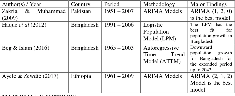
Table 1

Author(s) / Year Country Period Methodology Major Findings

Zakria & Muhammad (2009)

Pakistan 1951 – 2007 ARIMA Models ARIMA (1, 2, 0) is the best model Haque et al (2012) Bangladesh 1991 – 2006 Logistic

Population Model (LPM)

The LPM has the best fit for population growth in Bangladesh

Beg & Islam (2016) Bangladesh 1965 – 2003 Autoregressive

Time Trend

Model (ATTM)

Downward

population growth for Bangladesh for the extended period up to 2043

Ayele & Zewdie (2017) Ethiopia 1961 – 2009 ARIMA Models ARIMA (2, 1, 2) Model is the best model

MATERIALS & METHODS

ARIMA Models

ARIMA models are often considered as delivering more accurate forecasts then econometric techniques (Song et al, 2003b). ARIMA models outperform multivariate models in forecasting performance (du Preez & Witt, 2003). Overall performance of ARIMA models is superior to that of the naïve models and smoothing techniques (Goh & Law, 2002). ARIMA models were developed by Box and Jenkins in the 1970s and their approach of identification, estimation and diagnostics is based on the principle of parsimony (Asteriou & Hall, 2007). The general form of the ARIMA (p, d, q) can be represented by a backward shift operator as:

∅(𝐵)(1 − 𝐵)𝑑_𝑃𝑂𝑃

𝑡= 𝜃(𝐵)𝜇𝑡… … … . … … … … . . [1]

Where the autoregressive (AR) and moving average (MA) characteristic operators are:

∅(𝐵) = (1 − ∅1𝐵 − ∅2𝐵2− ⋯ − ∅𝑝𝐵𝑝) … … … . … … … [2]

𝜃(𝐵) = (1 − 𝜃1𝐵 − 𝜃2𝐵2− ⋯ − 𝜃𝑞𝐵𝑞) … … … . . [3]

(4)

(1 − 𝐵)𝑑_𝑃𝑂𝑃

𝑡 = ∆𝑑𝑃𝑂𝑃𝑡… … … . … … … … . . [4]

Where ∅ is the parameter estimate of the autoregressive component, 𝜃 is the parameter estimate

of the moving average component, ∆ is the difference operator, d is the difference, B is the

backshift operator and 𝜇_𝑡 is the disturbance term.

The Box – Jenkins Methodology

The first step towards model selection is to difference the series in order to achieve stationarity. Once this process is over, the researcher will then examine the correlogram in order to decide on the appropriate orders of the AR and MA components. It is important to highlight the fact that this procedure (of choosing the AR and MA components) is biased towards the use of personal judgement because there are no clear – cut rules on how to decide on the appropriate AR and MA components. Therefore, experience plays a pivotal role in this regard. The next step is the estimation of the tentative model, after which diagnostic testing shall follow. Diagnostic checking is usually done by generating the set of residuals and testing whether they satisfy the characteristics of a white noise process. If not, there would be need for model re – specification and repetition of the same process; this time from the second stage. The process may go on and on until an appropriate model is identified (Nyoni, 2018).

Data Collection

This study is based on 58 observations of annual total population in Yemen. All the data was gathered from the World Bank.

Diagnostic Tests & Model Evaluation

[image:4.612.78.552.448.708.2]

Stationarity Tests: Graphical Analysis

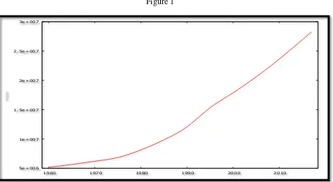
Figure 1

5e+006 1e+007 1.5e+007 2e+007 2.5e+007 3e+007

(5)

Figure 1 above indicates that the Yemen POP variable is not stationary since it is trending upwards over the period 1960 – 2017. This basically shows that the mean and varience of POP is changing over time.

[image:5.612.78.550.172.461.2]

The Correlogram in Levels

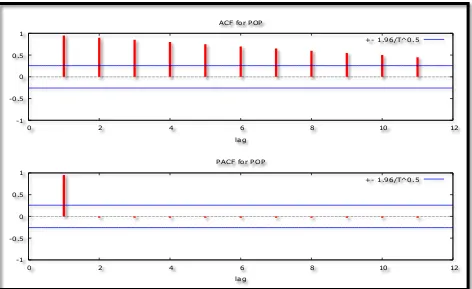
Figure 2

The ADF Test

Table 2: Levels-intercept

Variable ADF Statistic Probability Critical Values Conclusion

POP 0.289857 0.9754 -3.574446 @1% Not stationary

-2.923780 @5% Not stationary -2.599925 @10% Not stationary Table 3: Levels-trend & intercept

POP -2.521067 0.3171 -4.161144 @1% Not stationary

-3.506374 @5% Not stationary -3.183002 @10% Not stationary Table 4: without intercept and trend & intercept

-1 -0.5 0 0.5 1

0 2 4 6 8 10 12

lag ACF for POP

+- 1.96/T^0.5

-1 -0.5 0 0.5 1

0 2 4 6 8 10 12

lag PACF for POP

(6)

POP 0.924660 0.9028 -2.614029 @1% Not stationary -1.947816 @5% Not stationary -1.612492 @10% Not stationary

The Correlogram (at 1st Differences)

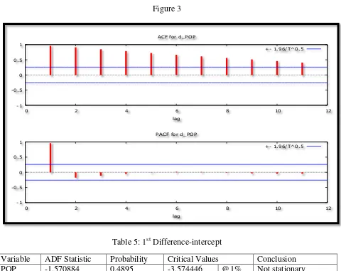
[image:6.612.71.551.134.515.2]

Figure 3

Table 5: 1st Difference-intercept

[image:6.612.64.549.454.708.2]

-2.923780 @5% Not stationary -2.599925 @10% Not stationary Table 6: 1st Difference-trend & intercept

-3.506374 @5% Not stationary -3.183002 @10% Not stationary Table 7: 1st Difference-without intercept and trend & intercept

POP 0.745622 0.8721 -2.614029 @1% Not stationary

-1.947816 @5% Not stationary -1.612492 @10% Not stationary

-1 -0.5 0 0.5 1

0 2 4 6 8 10 12

lag ACF for d_POP

+- 1.96/T^0.5

-1 -0.5 0 0.5 1

0 2 4 6 8 10 12

lag PACF for d_POP

(7)

Figures above, i.e. 2 and 3 and tables above, i.e. 2 to 7 show that the Yemen POP series is not stationary in levels and in first differences.

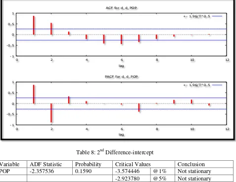
The Correlogram in (2nd Differences)

[image:7.612.74.551.165.533.2]

Figure 4

Table 8: 2nd Difference-intercept

[image:7.612.67.547.443.713.2]

-2.923780 @5% Not stationary -2.599925 @10% Not stationary Table 9: 2nd Difference-trend & intercept

-3.506374 @5% Not stationary -3.183002 @10% Not stationary Table 10: 2nd Difference-without intercept and trend & intercept

-1.947816 @5% Not stationary -1.612942 @10% Not stationary

-1 -0.5 0 0.5 1

0 2 4 6 8 10 12

lag ACF for d_d_POP

+- 1.96/T^0.5

-1 -0.5 0 0.5 1

0 2 4 6 8 10 12

lag PACF for d_d_POP

(8)

Figure 4 and tables 8 – 10 illustrate that the Yemen POP series is not stationary even after taking second differences. This is a feature of sharply upwards trending series. However, the researcher will assume that the Yemen POP series is I (2).

Evaluation of ARIMA models (without a constant)

Table 11

Model AIC U ME MAE RMSE MAPE

ARIMA (1, 2, 1) 1162.581 0.01867 852.93 4689.2 7190.2 0.039448

ARIMA (1, 2, 0) 1208.130 0.028836 1195.5 6701.8 11151 0.056933

ARIMA (0, 2, 1) 1231.736 0.039183 5408.1 9985.4 13732 0.087434

ARIMA (2, 2, 1) 1116.738 0.012974 1512.3 3443.9 4623.2 0.030322

ARIMA (3, 2, 1) 1110.82 0.011763 887.32 3099.5 4289.2 0.027383

ARIMA (4, 2, 1) 1112.799 0.011756 879.11 3098 4288.4 0.027362

ARIMA (5, 2, 1) 1114.665 0.011713 854.37 3088.1 4283.3 0.027226

ARIMA (6, 2, 1) 1108.818 0.011007 710.86 2837.3 3966.3 0.025118

ARIMA (2, 2, 0) 1130.302 0.015377 2065.4 3956.9 5348.1 0.034992

ARIMA (3, 2, 0) 1108.868 0.011769 912.06 3107.3 4290.7 0.027432

ARIMA (4, 2, 0) 1110.829 0.011765 892.61 3101.3 4289.4 0.027397

ARIMA (5, 2, 0) 1112.668 0.011713 855.65 3088.3 4283.4 0.027228

ARIMA (6, 2, 0) 1114.631 0.011716 839.45 3084.7 4282.1 0.0272

ARIMA (7, 2, 1) 1099.283 0.0099294 930.84 2545 3538 0.022635

ARIMA (8, 2, 1) 1096.748 0.0092395 607.33 2431.9 3381.7 0.021513

ARIMA (9, 2, 1) 1098.732 0.009407 606.54 2434.6 3381.1 0.021536

ARIMA (10, 2, 1) 1096.387 0.0089871 554.07 2333.6 3238.8 0.020784

ARIMA (7, 2, 0) 1105.442 0.010784 1092.2 2793.7 3839.2 0.024656

ARIMA (8, 2, 0) 1095.844 0.0093616 686.29 2506.3 3416 0.022023

ARIMA (9, 2, 0) 1097.398 0.0092945 649.04 2464.4 3401.9 0.021725

ARIMA (10, 2, 0) 1095.318 0.009041 553.2 2404.8 3269.8 0.021202

A model with a lower AIC value is better than the one with a higher AIC value (Nyoni, 2018). Theil’s U must lie between 0 and 1, of which the closer it is to 0, the better the forecast method (Nyoni, 2018). The study will consider the minimum AIC in order to choose the best model for forecasting total population in Yemen. Therefore, the ARIMA (10, 2, 0) model is carefully selected.

Residual & Stability Tests

ADF Tests of the Residuals of the ARIMA (10, 2, 0) Model

Table 12: Levels-intercept

Rt -6.207839 0.0000 -3.584743 @1% Stationary

-2.928142 @5% Stationary

(9)

Rt -6.241041 0.0000 -4.175640 @1% Stationary

-3.186854 @10% Stationary Table 14: without intercept and trend & intercept

Rt -6.203022 0.0000 -2.617364 @1% Stationary

Tables 11 – 13 indicate that the residuals of the chosen optimal model, the ARIMA (10, 2, 0) model; are stationary.

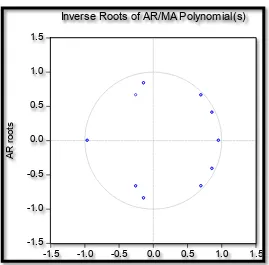
[image:9.612.171.440.293.558.2]

Stability Test of the ARIMA (10, 2, 0) Model

Figure 5

Since the corresponding inverse roots of the characteristic polynomial lie in the unit circle, it shows that the chosen ARIMA (10, 2, 0) model is stable.

FINDINGS

Descriptive Statistics

Table 15

Description Statistic

Mean 13471000

-1.5 -1.0 -0.5 0.0 0.5 1.0 1.5

A

R

r

o

ts

(10)

Median 11287000

Minimum 5172100

Maximum 28250000

Standard deviation 7277100

Skewness 0.53191

Excess kurtosis -1.0821

As shown above, the mean is positive, i.e. 13471000. The wide gap between the minimum (i.e 5172100) and the maximum (i.e. 28250000) is consistent with the observation that the Yemen POP series is sharply trending upwards over the period 1960 – 2017. The skewness is 0.53191 and the most essential characteristic is that it is positive, meaning that the Yemen POP series is positively skewed and non-symmetric. Excess kurtosis is -1.0821; showing that the Yemen POP series is not normally distributed.

[image:10.612.68.546.70.160.2]

Results Presentation1

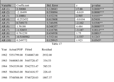
Table 16

ARIMA (10, 2, 0) Model:

∆2_𝑃𝑂𝑃

𝑡−1= 2.3∆2𝑃𝑂𝑃𝑡−1− 2.2∆2𝑃𝑂𝑃𝑡−2+ 1.1∆2𝑃𝑂𝑃𝑡−3− 0.3∆2𝑃𝑂𝑃𝑡−4+ 0.7∆2𝑃𝑂𝑃𝑡−5+ 1.2∆2𝑃𝑂𝑃𝑡−6

− 1.3∆2_𝑃𝑂𝑃

𝑡−7+ 0.8∆2𝑃𝑂𝑃𝑡−8− 0.5∆2𝑃𝑂𝑃𝑡−9+ 0.2∆2𝑃𝑂𝑃𝑡−10… … … . … . . [5]

Variable Coefficient Std. Error z p-value

AR (1) 2.30088 0.128683 17.88 0.0000***

AR (2) -2.18499 0.330094 -6.619 0.0000***

AR (3) 1.10861 0.432238 2.565 0.0103**

AR (4) -0.252452 0.413608 -0.6104 0.5416

AR (5) 0.749173 0.346496 -2.162 0.0306**

AR (6) 1.56186 0.348357 4.484 0.0000***

AR (7) -1.32833 0.416786 -3.187 0.0014***

AR (8) 0.761239 0.434938 1.75 0.0801*

AR (9) -0.5100562 0.332144 -1.537 0.1243

AR (10) 0.249772 0.129915 1.923 0.0545*

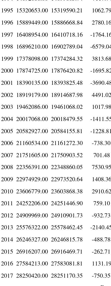
Table 17

Year Actual POP Fitted Residual

1962 5351799.00 5348867.00 2932.00

1963 5446063.00 5445728.47 334.53

1964 5543339.00 5542753.47 585.53

1965 5643643.00 5643416.57 226.43

1966 5748588.00 5746720.63 1867.37

1

[image:10.612.66.548.351.699.2]

(11)

1967 5858638.00 5859834.08 -1196.08

1968 5971407.00 5972987.95 -1580.95

1969 6083619.00 6083437.11 181.89

1970 6193810.00 6193050.00 760.00

1971 6300554.00 6301214.18 -660.18

1972 6407295.00 6403391.57 3903.43

1973 6523452.00 6520740.43 2711.57

1974 6661566.00 6658591.55 2974.45

1975 6830692.00 6829798.69 893.31

1976 7034868.00 7034424.78 443.22

1977 7271872.00 7270659.47 1212.53

1978 7536764.00 7533607.38 3156.62

1979 7821552.00 7821651.41 -99.41

1980 8120497.00 8118534.00 1963.00

1981 8434017.00 8430492.58 3524.42

1982 8764621.00 8766017.45 -1396.45

1983 9111097.00 9111929.64 -832.64

1984 9472170.00 9470725.54 1444.46

1985 9847899.00 9845673.74 2225.26

1986 10232733.00 10236725.18 -3992.18

1987 10628585.00 10618935.42 9649.58

1988 11051504.00 11045472.41 6031.59

1989 11523267.00 11519018.09 4248.91

1990 12057039.00 12058023.99 -984.99

1991 12661614.00 12657667.89 3946.11

1992 13325583.00 13334698.50 -9115.50

(12)

1994 14692686.00 14699803.74 -7117.74

1995 15320653.00 15319590.21 1062.79

1996 15889449.00 15886668.84 2780.16

1997 16408954.00 16410718.16 -1764.16

1998 16896210.00 16902789.04 -6579.04

1999 17378098.00 17374284.32 3813.68

2000 17874725.00 17876420.82 -1695.82

2001 18390135.00 18393825.48 -3690.48

2002 18919179.00 18914687.98 4491.02

2003 19462086.00 19461068.02 1017.98

2004 20017068.00 20018479.55 -1411.55

2005 20582927.00 20584155.81 -1228.81

2006 21160534.00 21161272.30 -738.30

2007 21751605.00 21750903.52 701.48

2008 22356391.00 22348860.05 7530.95

2009 22974929.00 22973520.64 1408.36

2010 23606779.00 23603868.38 2910.62

2011 24252206.00 24251446.90 759.10

2012 24909969.00 24910901.73 -932.73

2013 25576322.00 25578462.45 -2140.45

2014 26246327.00 26246815.78 -488.78

2015 26916207.00 26916469.71 -262.71

2016 27584213.00 27583081.81 1131.19

2017 28250420.00 28251170.35 -750.35

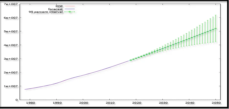
[image:12.612.70.290.82.647.2]

Forecast Graph

(13)

[image:13.612.79.547.76.299.2]

Predicted Total Population

Table 18

Year Prediction Std. Error 95% Confidence Interval

2018 28916856.83 3238.390 28910509.71 - 28923203.96

2019 29586975.03 14299.445 29558948.64 - 29615001.43

2020 30263711.05 37517.680 30190177.75 - 30337244.35

2021 30948328.62 75847.822 30799669.62 - 31096987.62

2022 31640706.40 130910.209 31384127.10 - 31897285.69

2023 32339818.67 201672.643 31944547.56 - 32735089.79

2024 33044077.24 285054.080 32485381.51 - 33602772.97

2025 33752117.98 377405.576 33012416.65 - 34491819.32

2026 34463290.13 475936.523 33530471.68 - 35396108.57

2027 35177349.52 578933.659 34042660.40 - 36312038.64

2028 35893925.15 686031.832 34549327.46 - 37238522.83

2029 36612393.63 797904.907 35048528.75 - 38176258.51

2030 37331924.63 915740.360 35537106.50 - 39126742.75

2031 38051683.51 1040531.265 36012279.71 - 40091087.32

0 1e+007 2e+007 3e+007 4e+007 5e+007 6e+007 7e+007

1980 1990 2000 2010 2020 2030 2040 2050 POP

(14)

2032 38771229.59 1172958.543 36472273.09 - 41070186.09

2033 39490886.77 1313396.527 36916676.88 - 42065096.66

2034 40211663.74 1462151.525 37345899.41 - 43077428.07

2035 40934842.84 1619580.113 37760524.15 - 44109161.53

2036 41661476.96 1786231.211 38160528.12 - 45162425.80

2037 42392006.79 1962637.153 38545308.65 - 46238704.92

2038 43126083.89 2149071.303 38913981.53 - 47338186.24

2039 43862755.64 2345283.336 39266084.77 - 48459426.51

2040 44600882.06 2550531.040 39601933.08 - 49599831.04

2041 45339561.29 2763726.132 39922757.60 - 50756364.97

2042 46078344.46 2983799.613 40230204.68 - 51926484.24

2043 46817238.76 3209995.197 40525763.79 - 53108713.74

2044 47556512.34 3442079.201 40810161.07 - 54302863.60

2045 48296443.73 3680269.369 41083248.31 - 55509639.14

2046 49037142.47 3925067.308 41344151.91 - 56730133.03

2047 49778552.27 4176985.245 41591811.63 - 57965292.92

2048 50520568.36 4436373.791 41825435.51 - 59215701.21

2049 51263188.00 4703319.215 42044851.73 - 60481524.27

2050 52006578.29 4977712.504 42250441.05 - 61762715.52

Table 17 shows the actual total population of Yemen, the fitted one as well as the residuals. The striking feature of table 17 is that the residuals are quite small, confirming the accuracy of the selected optimal model, the ARIMA (10, 2, 0) model as already hinted by the forecast evaluation statistics in table 11 above. Figure 6 (with a forecast range from 2018 – 2050) and table 18, clearly show that Yemen’s total population is set to continue rising rapidly, in the next 3 decades. With a 95% confidence interval of 42250441 to 61762716 and a projected total population of 52006578 by 2050, the chosen ARIMA (10, 2, 0) model is consistent with the population projections by the UN (2015) which forecasted that Yemen’s population will be approximately 47170000 by 2050.

Policy Implications

(15)

ii. The predicted increase in total population in Yemen justifies the need for more and bigger companies to provide for the anticipated increase in demand for goods and services in Yemen.

iii. The government of Yemen should take action so as to improve health service delivery in the country in order to ensure a healthier society, particularly in light of such a likely increase in total population.

iv. The consequences of the armed conflict on the Yemeni people are a fundamental concern. The need for political stability cannot be undermined in Yemen. The Yemen-Saudi Arabia conflict just liked any other armed conflict in Yemen; is condemned at all costs. Without political stability, Yemen’s expected increase in total population is a threat to Yemen herself especially in light of the lack of the most basic survival means and high food prices currently obtaining in the country.

CONCLUSION

The study shows that the ARIMA (10, 2, 0) model is not only stable but also the most suitable model to forecast total population in Yemen for the next 3 decades. The model predicts that by 2050, Yemen’s total population would be approximately, 52 million people. This is a warning signal to policy makers in Yemen, particularly with regards to infrastructural development, e.g schools and hospitals. These findings are essential for the government of Yemen, especially when it comes to long-term planning.

REFERENCES

[1] Asteriou, D. & Hall, S. G. (2007). Applied Econometrics: a modern approach, Revised Edition, Palgrave MacMillan, New York.

[2] Ayele, A. W & Zewdie, M. A (2017). Modeling and forecasting Ethiopian human population size and its pattern, International Journal of Social Sciences, Arts and Humanities, 4 (3): 71 – 82.

[3] Beg, A. B. M. R. A & Islam, M. R (2016). Forecasting and modeling population growth of Bangladesh, American Journal of Mathematics and Statistics, 6 (4): 190 – 195.

[4] Dominic, A., Oluwatoyin, M. A., & Fagbeminiyi, F. F (2016). The determinants of population growth in Nigeria: a co-integration approach, The International Journal of Humanities and Social Studies, 4 (11): 38 – 44.

[5] Du Preez, J. & Witt, S. F. (2003). Univariate and multivariate time series forecasting: An application to tourism demand, International Journal of Forecasting, 19: 435 – 451.

[6] Goh, C. & Law, R. (2002). Modeling and forecasting tourism demand for arrivals with stochastic non-stationary seasonality and intervention, Tourism Management, 23: 499 – 510.

(16)

[8] Jamada II (2005). Country Profile – Yemen, Republic of Yemen.

[9] MOPHP-SCO (Yemen)-PAPFAM & ICFI (2015). Yemen National Health and Demographic Survey 2013, Rockville, Maryland.

[10] Nyoni, T (2018). Modeling and Forecasting Inflation in Kenya: Recent Insights from ARIMA and GARCH analysis, Dimorian Review, 5 (6): 16 – 40.

[11] Nyoni, T (2018). Modeling and Forecasting Naira / USD Exchange Rate in Nigeria: a Box – Jenkins ARIMA approach, University of Munich Library – Munich

Personal RePEc Archive (MPRA), Paper No. 88622.

[12] Nyoni, T. (2018). Box – Jenkins ARIMA Approach to Predicting net FDI inflows in Zimbabwe, Munich University Library – Munich Personal RePEc Archive (MPRA), Paper No. 87737.

[13] Song, H., Witt, S. F. & Jensen, T. C. (2003b). Tourism forecasting: accuracy of alternative econometric models, International Journal of Forecasting, 19: 123 – 141.

[14] Tartiyus, E. H., Dauda, T. M., & Peter, A (2015). Impact of population growth on economic growth in Nigeria, IOSR Journal of Humanities and Social Science (IOSR-JHSS), 20 (4): 115 – 123.

[15] Todaro, M & Smith, S (2006). Economic Development, 9th Edition, Vrinda

Publications, New Delhi.

[16] United Nations (2015). World Population Prospects: The 2015 Revision, Key Findings and Advance Tables, Department of Economic and Social Affairs, Population Division, Working Paper No. ESA/P/WP/241.

[17] Zakria, M & Muhammad, F (2009). Forecasting the population of Pakistan using ARIMA models, Pakistan Journal of Agricultural Sciences, 46 (3): 214 – 223.