Multiple Days Ahead Realized Volatility Forecasting: Single, Combined and Average Forecasts

Munich Personal RePEc Archive

Multiple Days Ahead Realized Volatility

Forecasting: Single, Combined and

Average Forecasts

Degiannakis, Stavros

Department of Economic and Regional Development, Panteion

University, 136 Syggrou Av., Athens, 176 71, Greece

2018

Online at

https://mpra.ub.uni-muenchen.de/96272/

1

M u l t i p l e D a y s A h e a d R e a l i z e d V o l a t i l i t y F o r e c a s t i n g :

S i n g l e , C o m b i n e d a n d A v e r a g e F o r e c a s t s

Stavros Degiannakis

Department of Economic and Regional Development, Panteion University, 136 Syggrou Av., Athens, 176 71, Greece, email: [email protected]

A b s t r a c t

The task of this paper is the enhancement of realized volatility forecasts. We investigate

whether a mixture of predictions (either the combination or the averaging of forecasts) can

provide more accurate volatility forecasts than the forecasts of a single model.We estimate

long-memory and heterogeneous autoregressive models under symmetric and asymmetric

distributions for the major European Union stock market indices and the exchange rates of

the Euro.

The majority of models provide qualitatively similar predictions for the next trading day’s

volatility forecast. However, with regard to the one-week forecasting horizon, the

heterogeneous autoregressive model is statistically superior to the long-memory framework.

Moreover, for the two-weeks-ahead forecasting horizon, the combination of realized

volatility predictions increases the forecasting accuracy and forecast averaging provides

superior predictions to those supplied by a single model. Finally, the modeling of volatility

asymmetry is important for the two-weeks-ahead volatility forecasts.

K e y w o r d s :averaging forecasts, combining forecasts, heterogeneous autoregressive,

intra-day data, long memory, model confidence set, predictive ability, realized volatility, ultra-high

frequency.

2

1. Introduction

Undoubtedly, ultra-high frequency financial data have been valuable in estimating

and forecasting volatility more accurately. The long-memory autoregressive and the

heterogeneous autoregressive models are representative methods of volatility forecasting.

The literature provides strong evidence that ARFIMA models introduced by Granger

(1980), produce superior forecasts relative to those produced by conditional volatility

GARCH models that are based on daily returns. Due both to the long memory property of

volatility as well as its high persistence, the ARFIMA specification is suitable for estimating

realized volatility. Among others, Andersen et al. (2003), Chiriac and Voev (2011), Deo et al.

(2005), Koopman et al. (2005), Martens and Zein (2002), Pong et al. (2004) have applied

various extensions of ARFIMA models to ultra-high frequency-based volatility measures.

The structure of the Heterogeneous Autoregressive model of realized volatility is

based on the heterogeneous market hypothesis (Müller et al., 1997), which states that in

financial markets, investors (ultra-high frequency algorithmic traders, inter-day investors,

institutional investors trading on a monthly basis, etc.) interact at different frequencies. Thus,

the HAR model is able to accommodate the heterogeneous beliefs of traders; different types

of market participants drive volatility at different frequencies. Andersen et al. (2007) show

that volatility for equity and bond futures is adequately expressed by a HAR-GARCH model.

In forecasting ultra-high frequency constructed volatility, various extensions of the HAR

model have been applied by Chen and Ghysels (2011), Clements et al. (2008), Corsi and

Reno (2012), Hua and Manzan (2013), Prokopczuk et al. (2015), Sevi (2014) and

Degiannakis and Filis (2017). In general, the literature provides evidence in favor of the HAR

model compared to other models such as the plain autoregressive model, the MIDAS model

of Ghysels et al. (2007), the HEAVY model of Shephard and Sheppard (2010), the ARFIMA

model, etc.

Apart from modelling information of realized volatility from the past, an alternative

approach is to extract the predictive information from the futures market. Such techniques

have been employed mainly by policy institutions1, which are looking for the market expectations of the exogenous variables required for their macroeconomic model

frameworks. Alquist and Kilian (2010) provided an interesting analysis of oil price forecasts

based on futures prices. Their study showed that futures are not the most accurate predictor of

the spot price of crude oil; even no-change forecasts tend to be more accurate.

1_{The interested reader is referred to Svensson (2005) for the European Central Bank, and to the IMF (2007) for}

3

Additionally, the implied volatility extracted from the option prices has been

considered as an alternative source of measuring investor sentiment with regard to market

volatility. Koopman et al. (2005) showed that models based on realized volatility (i.e.

ARFIMA models) outperform models based on implied volatility. On the other hand,

Fleming et al. (1995), Christensen and Prabhala (1998), Fleming (1998), Blair et al. (2001),

Giot (2003), Degiannakis (2008) and Frijns et al. (2010) provided evidence that implied

volatility is more informative when stock market volatility is being investigated.

Although model-averaging methods for forecasting purposes date back to the works of

Bates and Granger (1969), Granger and Newbold (1977) and Granger and Ramanathan

(1984), the combination of volatility forecasts has not been broadly studied. Liu and Maheu

(2009) and Wang et al. (2016) have investigated the impact of model averaging on realized

volatility prediction accuracy, while Amendola and Storti (2008) and Hu and Tsoukalas

(1999) have examined the performance of combining forecasts estimated from conditional

volatility models (i.e. based on daily data). However, the performance of combined forecasts

has not been explored for ultra-high frequency based volatility estimates.

This paper studies whether the combination or the averaging of realized volatility

predictions increases forecasting accuracy. It brings to light two strands of mixed predictions

(i) selecting forecasts from a set of candidate models according to an evaluation criterion; and

(ii) the averaging of forecasts.

This forecasting evaluation exercise is not limited to one-day-ahead forecasts, as

multiple-days-ahead forecasts (i.e. one-week and two-weeks-ahead forecasting horizons)

gather investor interest as well. Moreover, we investigate the predictive accuracy under four

different distributions for the standardized unpredictable component of the models. Briefly,

our results conclude that: 1) The heterogeneous autoregressive framework works better than

the long memory framework. 2) The averaged models provide superior forecasts compared to

those of single models. 3) The modeling of volatility asymmetry is crucial in forecasting the

ten-days-ahead realized volatility. 4) The combination of volatility forecasts according to the

statistical properties of forecast errors provides us with more accurate two-weeks-ahead

volatility forecasts compared to forecasts from a single model.

The remainder of this study is structured as follows. Section 2 describes the

estimation of the realized volatility measures, section 3 provides information for the dataset

of the 3 stock market indices and the 3 exchange rates, while sections 4 and 5 demonstrate the

ARFIMA and HAR estimated models and the relative forecast specifications for one-day and

4 according to model selection criteria and methods of computing the model-average forecasts,

respectively. Section 8 describes a unified framework for the evaluation of all predictive

methods. Section 9 reports the empirical results and suggests when we should apply the

volatility forecasts of a single model, a combination of models, or the average forecast from a

set of models. Section 10 concludes the paper and suggests areas for further research.

2. The Realized Volatility Measure

The financial literature assumes that the instantaneous logarithmic price

p

 

t

of an asset

follows a diffusion process

d

log

p

     

t





t

dW

t

, where



 

t

is volatility and

W

 

t

is the Wiener process. The integrated variance _ IV_

t t

2 , 1 

 is the actual, but unobservable, variance over

the interval

 

t1,t for which we seek a proxy measure to estimate. Assuming that the number

of points in time tends to infinity,



, we are able to approximate the integrated variance

as _{ } 



 



 



 

   

 

 

 

 t

t t

t t

t IV b

a t dt t dt t dt

1 3

2 2

1

2 2

2 2

, ... . The realized volatility for the time

interval

 

t1,t which is partitioned in



equidistance points,

 

















 1

2

, 1

1t j

log

t

log

t

t

P

j

P

j

RV

converges in probability towards the integrated volatility2,

orp



RV t t



 t IVt 2

,

, 1

1

lim _



_

  . Accuracy improves as the number of sub-intervals increases, or as

 



, but on the other hand, at a high sampling frequency, such as sf 0, market friction

is a source of noise due to market microstructure features (i.e. discreteness of the data,

transaction costs, properties of the trading mechanism, bid-ask spreads, etc.). Thus, realized

volatility is constructed in the highest sampling frequency which the intra-day autocovariance

minimizes3; see e.g. Andersen et al. (2006), and Degiannakis and Floros (2015). The

2_{The p}

 

_{t is the latent efficient price, whereas} j t

P is the observed price. The unobserved distance between p

 

t

and Ptjis the market microstructure noise. There exist a number of estimators for the integrated volatility that

possess asymptotical properties which are robust for microstructure noise and jumps. However, Sévi (2014) and Prokopczuk et al. (2015) provided empirical evidence that the modelling of jumps does not improve the forecast accuracy of the simple HAR-RV model. Thus, we construct the realized volatility estimates without taking into consideration the presence of jumps.

3 _{The inter-day variance can be decomposed into the intra-day variance,}  

t

RV , and the intra-day autocovariancesytiyt_i_j:

 

 



   

 1

1 1

2

2  



j i j ti ti j t

t RV y y

5 sequence of the sampling prices is constructed according to the previous tick method4 of

Wasserfallen and Zimmermann (1985).

In order to incorporate estimates of asset prices during the hours that the stock

markets are closed to volatility, we take into consideration Hansen and Lunde's (2005)

method of combining intraday volatility with closed-to-open inter-day volatility. Hansen and

Lunde proposed the construction of the realized volatility measure as a weighted combination

of RV_t,t

1 with inter-day volatility during the time that the market is closed;





2

1

log log

1  t

t P

P . Hence, we estimate

 

































 1

2 2

2 1

1

log

t1

log

t j

log

t

log

t 1

t

P

P

P

j

P

j

RV

, such as_{ }



  _2 _{, }



2

, 1

2 1

min IV

t t t

RV

E   _



  . As

the _ IV_ t t

2 , 1 

 is unobservable, Hansen and Lunde (2005) provide the analytic solution of

 

 

 





1, 2

V

RV

t

min

instead of _{ }



  _2 _{, }



2

, 1

2 1

min IV

t t t

RV

E   _



  , as both functions lead to the same solution.

Hence, we minimize the squared distance between the realized volatility measure and

integrated volatility, avoiding the need to define a specific relation betweenefficient prices

and market microstructure noise.

3. Dataset - FTSE100, DAX30, CAC40 and Euro Exchange Rates

The database is made up of the three most liquid euro exchange rates (with the Pound, the

Dollar and the Yen) and the three major European stock indices (FTSE100, DAX30,

CAC40). The Euro, the Pound, the Dollar and the Yen are the four most tradable currencies.

The blue-chip FTSE 100 from the London Stock Exchange, has a market cap of €1.8 trillion,

the DAX30 (a market cap of €1 trillion) from the Deutsche Boerse group, is Germany's prime

index featuring many of Europe's biggest companies, and the CAC40 (market cap of €1.2

trillion) represents a capitalization-weighted measure of the 40 most significant companies

listed on the Euronext Paris (formerly Paris Bourse).

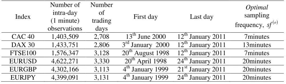
Table 1 presents information for the one-minute intra-day data of the FTSE100,

DAX30, and CAC40 indices, as well as for the exchange rates of Euro with the British

Pound, the US Dollar and the Japanese Yen. The data are filtered for detecting data errors due

to computer technical failures, typing errors, sequences of zero or non-available prices due to

databases crashes, etc. Weekends and fixed and moving holidays with thin trading activity

have been deleted. The selection of the optimal sampling frequency sf o , is based on a

4 _{Based on the previous tick method (e.g. employ the most recently published price), we obtain a volatility}

6 off between accuracy and potential biases due to market microstructure frictions (last column

of Table 1)5. The interday adjustment of Hansen and Lunde (2005) is taken into

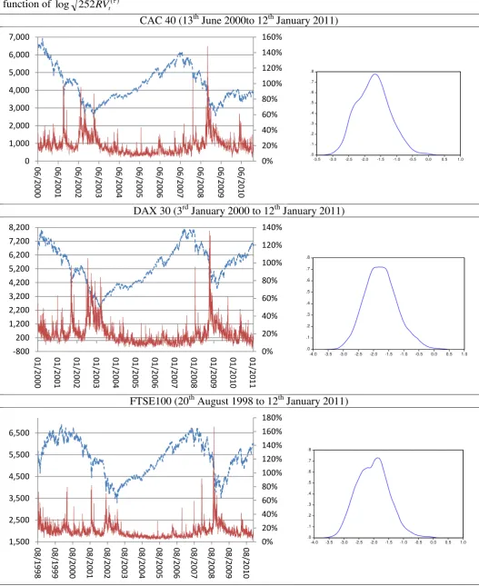
consideration. Figure 1 plots the annualized realized volatilities, 252RVt  and the

empirical density functions of log 252RVt  .

[Insert Table 1 about here]

[Insert Figure 1 About here]

The logarithmic transformation of realized volatility has an ogive empirical

distribution which approximates the Gaussian distribution. The average value of the

annualized standard deviation for the three stock indices is 18.8% (see Table 2). The mean of

the annualized standard deviation for the three euro exchange rates is 10.1%. The maximum

annualized volatility observed for the FTSE100 index was 167%, on Friday, October 10,

2008 (Global financial crisis of October 2008). On Friday, October 10, the stock markets

crashed across Europe and Asia. London, Paris and Frankfurt dropped 10% in the first hour

of trading and this also happened when Wall Street opened for trading. Since 1987, global

markets have experienced some of their worst weeks in memory, and indeed in some cases,

since the Wall Street Crash of 1929. The median value of annualized volatility ranges from

13.3% for the FTSE100 to 17.8% for the CAC40. On the other hand, realized standard

deviations of exchange rates do not fluctuate over time at a similar magnitude. The median

value of annualized volatility ranges from 7.5% for the Euro/Pound rate to 10.2% for the

Euro/Yen rate. Maximum annualized volatility is observed for the Euro/Yen exchange rate to

74%, on October 24, 2008 (when recession fears caused great turbulence in the Euro/Yen

rate). Table 3 provides descriptive statistics of the annualized logarithmic realized volatility.

Sample skewness is positive in all cases. The average of the skewness of log-standard

deviations across the stock indices decreases to 0.3 compared to 2.9 for the realized standard

deviations. As far as kurtosis is concerned, the average value for the log-volatilities, across

the stock indices, is 3.1 compared to 19.5 for the realized standard deviations. Therefore,

although the kurtosis of the indices exceeds the normal value of three, the logarithmic

transformation case is obviously much closer to the assumption of normality. Normality

approximation is very good for the log-volatilities of the exchange rates as well.

[Insert Table 2 about here]

[Insert Table 3 about here]

7

4. Estimation of the Models

We proceed to an estimation of two widely accepted model frameworks for the

annualized logarithmic realized volatility, log 252RVt  . The first framework is the

Autoregressive Fractionally Integrated Moving Average, or the ARFIMA model with

time-varying conditional innovations. The ARFIMA, initially developed by Granger (1980) and

Granger and Joyeux (1980), captures the long-memory property of dependent variables. The

time-variation and clustering that the volatility of realized volatility exhibits is modeled by

extending the ARFIMA to the ARFIMA-GARCH framework proposed by Baillie et al.

(1996). The ARFIMA(k,d,l)-GARCH(p,q) model for log 252RVt  is defined as:

 









 





 



 

 



0,1;



, ~ 1 252 log 1 1 2 2 0 2 0 θ f z h L B L A a h z h L D RV L L C t t t t t t t t t d               (1)

where

 



  k i i iL c L C 1 ,

 



  l i i iL d L D 1 ,

 



  q i i iL a L A 1 ,

 



  p i i iL b L B 1

are polynomials,

f



.

is

the density function of zt (with E

 

zt 0, V

 

zt 1, θis the vector of the parameters which

define f ) and d,0,c1,...,ck,d1,...,dl,a1,...,aq,b1,...,bp,θare the parameters to be estimated.

The 2

t

h can be considered as an estimate of the integrated quarticity _t2 IQ .6

The second framework is the Heterogeneous Autoregressive, or HAR model with

time-varying conditional innovations; e.g. of Corsi et al. (2008) and Corsi (2009). The basic

idea is that market participants have a different perspective of their investment horizon. The

HAR-RV-GARCH(p,q) model is an autoregressive structure of the volatilities realized over

different interval sizes:

6 _{The asymptotic volatility of volatility,}

t IQt 2

, 1

 , is termed integrated quarticity:   



 

    t t IQ t

t t dt

1 4 2

,

1 2 , as

 

 

2

 

 

0,1 1

4 1

2 ,

1 tdt t dt N

RV d t t t t t

t  

8

     

 

 

 



0,1,;



, ~ , , 252 log 22 252 log 5 252 log 252 log 2 2 0 2 22 1 1 3 5 1 1 2 1 1 0 θ f z h L B L A a h z h RV w RV w RV w w RV t t t t t t t t j j t j j t t t                     





              (2)

where

 



  q i i iL a L A 1 ,

 



  p i i iL b L B 1

are polynomials and w0,...,w3,a1,...,aq,b1,...,bp,θare the

parameters to be estimated.

For the 3 stock market indices and the 3 exchange rates, the

ARFIMA(0,d,1)-GARCH(1,1), ARFIMA(1,d,1)-ARFIMA(0,d,1)-GARCH(1,1), GARCH(1,1) and

HAR-RV-GARCH(0,1) model specifications with innovations (i.e. unexplained component of

conditional mean equation) that are i) normally distributed; z_t ~ N

 

0,1ii) Student t

distributed; z_t ~t



0,1;v



,iii) GED distributed z_t ~Ged



0,1;v



, and iv) skewed Student t

distributed; z_t ~skT



0,1;v,g



, are estimated. For z_t ~ N

 

0,1 , the density function is

 

 

_        2 exp 2 1 2 t t N z z f

 . Under the assumption of conditional Student t distributed

innovations z_t ~t



0,1;v



, the density function is:

 





  











2 1 2 2 1 2 2 2 1 ;                       t t t z z

f , for  2,7 (3)

where





.

is the gamma function. With conditional GED (Generalized Error Distribution or

Exponential Power distribution) distributed innovations

 

z_t T_t1~Ged



0,1;v



, the density

function is:  





_{ }



 



1 1 1 2 5 . 0 exp ;           v v t t GED z z

f ,  0, (4)

wherev is the tail-thickness parameter and  22

   

1 /31 .8For z_t ~skT



0,1;v,g



the density function is:9

7θ

 

_{v .}

8 _{For more technical details on the GED, readers are referred to Box and Tiao (1973) and Johnson et al. (1995).} 9 _{The skewed Student t distribution has been introduced by Fernandez and Steel (1998). Degiannakis (2004),}

9  













  











  



, , 2 1 2 2 2 2 1 2 1 2 2 2 2 1 , ; ₁ 1 2 1 1 1 2 1 1                                                              s z s z if if g sz g g s g sz g g s g z f t t t t t skT _               _  (5)

whereg and



are the asymmetry and tail parameters, respectively, of the distribution10







 

  





1



1



2 2

2

1     

 

     g g

 , and _s _g2 _g221_.

For each of the six time-series, 16 models are estimated; four model specifications

combined with four distributional assumptions. The lag orders k,d,l,p,q of the models have

been selected according to Schwarz's (1978) Bayesian information criterion.11Each of the 16

models is re-estimated every trading day t, for

T

~

days, where

T

~



1686, 1784, 2106, 2308, 2091, 2108 for the CAC40, DAX30, FTSE100, EURUSD, EURGBP and EURJPY realized

volatility series, respectively based on a rolling sample of constant size

T



=1000 days. For

the ARFIMA(1,d,1)-GARCH(1,1) model, the parameter vector to be estimated at each point

in time t is





₀             t

,

c

₁t

,

d

t

,

d

₁t

,

a

₀t

,

a

₁t

,

b

₁t





. Thus, for each model the vector of parameters is re-estimated every trading day, fortT,T1,...,TT~1 days, based on a rolling sample of

constant size T.

5. Realised Volatility Forecasting

The one-day-ahead adjusted logarithmic realized volatility,log



RVt 1|t



, and the ht1|t

for the ARFIMA(1,d,1)-GARCH(1,1) model are computed as





 



 



 







 



 

 





 





 

 





  tt t j j t t t t j j t t t t t t t t d L j d d j L j d d j RV c c RV | 1 0 | 1 1 1 1 0 | 1 1 1 252 log 1 252 log   





                                  (6) And

      2 | 1 2 | 1 0 |

1 tt

t t t t t t

t

a

a

b

h

h

_









.

The log



RVt1|t



for the ARFIMA(0,d,1)-GARCH(1,1) model is computed from eq.(6) for

  ₀

1  t

c . For the HAR-RV-GARCH(1,1) model we have:

10_θ

 

_v,g'.

11

10





   



 



 



 



 



 



, 252 log 22 252 log 5 252 log 252 log | 22 1 1 1 3 5 1 1 1 2 1 0 | 1 t t j j t t j j t t t t t t t RV w RV w RV w w RV     _                





         (7) and

      2 | 1 2 | 1 0 |

1 tt

t t t t t t

t

a

a

b

h

h

_









.

The ht1|t for the HAR-RV-GARCH(0,1) model is computed from eq.(7) for

  ₀

1  t

b .In

ARFIMA-GARCH and HAR-RV-GARCH frameworks, the dependent variable is

conditionally distributed as log 252RVt  |It 1~ f



t,ht2;θ





 , for It denoting the information

set available at time t and t referring to the conditional mean given It. Therefore, the

one-trading-day-ahead annualized realized volatility equals

      _  _{ }

1| 1| 21|

2 1 252

log exp

252RV_{t t} RV_{t t} h_{t t} .

The formulas for multiple-days-ahead realized volatility forecasts (n2) are constructed recursively based on Degiannakis et al. (2014). For example,log



RVtn|t



, and htn|t are

computed as: ARFIMA(1,d,1)-GARCH(1,1) model:





 



 



 





t n t t t t t n

t c c RV

RV _{| 0} 1 _{1 1} log 252 _|

252

log      (8)

      2 | 1 1 2 | 1 1 0

| t n t

t t n t t t t n

t

a

a

b

h

h

_







_{ }



_{ } . HAR-RV-GARCH(1,1) model:





   _log



₂₅₂



  _{5 log}



₂₅₂  



  _{22 log}



₂₅₂  



_,

252 log 22 1 1 3 5 1 1 2 | 1 1 0 |                





           j j n t t j j n t t t n t t t t n t RV w RV w RV w w RV 

 (9)

and

      2 | 1 1 2 | 1 1 0

| t n t

t t n t t t t n

t

a

a

b

h

h

_







_{ }



_{ } .

6. Combining Forecasts

In this section, we will investigate whether the combination of predictions can provide

more accurate volatility forecasts compared to the use of a specific single model. Let us

define that we have a set of M competing models. At each point in time we forecast the next

day’s volatility based on the model with the minimum forecast error. Specifically, we

investigate two rules (evaluation functions) for model selection based on the most recent

one-step-ahead forecast error, or t|t1 log



252RVt 

 

log 252RVt|t1





11 one-step-ahead standardized forecast error, or

1 | 1 | 1 |     t t t t t t h

z  . In other words, on day t1 we

estimate the M competing models, and for day t we compute the one-step-ahead forecasts.

For day t1 we forecast the volatility based on the model m with:  

 

m

t t M m 2 1 | ,..., 1

min_   (10)

or

 

 

m

t t M m z 2 1 | ,..., 1

min_  . (11)

The predicted squared forecast error, in eq. (10), is the most widely accepted criterion for

evaluating forecasting ability. The eq. (11) is the standardized predicted squared forecast

error, whose properties have been investigated by Degiannakis and Xekalaki (2005).

Consider a model with the generic form, which incorporates the models in eq. (1) and

eq. (2):

 



,



, 2 1 j t j t t t t t t t t g z y               η β x (12)

where η12 is a vector of parameters to be estimated, ~

 

0,1

. . . N z d i i

t ,



.

2

t

 represents the

conditional variance of t , and g



. is the functional form of the conditional variance. Under

the assumption of constancy of parameters over time, η1 η2 ...ηT η , the zt\t1 has an

asymptotic standard normal distribution, where





1

1 | 1 | 1 |      t  tt tt t

t y y

z  ,  1

1 1 |

    t t t

t

y x β and

1 |t t

 is the one-step-ahead conditional standard deviation.

If we have m1,2,...,Mcompeting models, we may compute the  m

t t z_|1.

Krishnamoorthy and Parthasarathy (1951) showed that if M variables jointly follow the

standard normal distribution, then the joint distribution of



     M



t t t t t

t z z

z | 1

2 1 | 1

1

| ,  ,...,  is the

Multivariate Gamma. Then the distribution function of _{ }



     M



t t t t t t M

m z z z

z | 1

2 1 | 1 1 | ,..., 1

1  min_ ,  ,...,  can be

used to compare the predictability of the M models. The cumulative distribution function of

 1

z is the minimum multivariate gamma (MMG) distribution (see Xekalaki and Degiannakis,

2005 and 2010). The single models are based on the statistical assumption that the

standardized residuals are i) normally, ii) Student t, iii) GED or iv) skewed Student t

12

distributed. On the other hand, the combined forecasts according to the

 

 m

t t M

m z

2 1 | ,..., 1

min_  criterion

for normally distributed standardized residuals have a known and explicitly derived

distribution form; the minimum multivariate gamma. Based on simulated evidence,

Degiannakis and Livada (2016) expanded the research on the non-normally distributed

standardized residuals. However, the combined forecasts according to the



 m



t t M m

2 1 | ,..., 1

min_  

criterion do not have a known distribution function, despite the fact that almost all the

forecasting evaluations conducted in the financial literature, are based on the

non-standardized residuals, t_|t₁. Hence, the combined forecasts according to the

 

  m t t M

m z

2 1 | ,..., 1

min_ 

criterion are compatible with the assumptions behind the each of the models that comprise it,

whereas this is not the case for the



 m



t t M m

2 1 | ,..., 1

min_   criterion.

7. Averaging Forecasts

Next, we proceed with model-average forecasts in order to assess whether the average

forecast could improve forecasting accuracy. We consider the model-average forecasts of all

the models with the same distributional assumption:

 



 

 

  

M

m

m t n t distr

t n

t M RV

AV

1

| 1

| 252 , (13)

whereM 4 and distrN,t,Ged,skT denotes the conditional distribution of the models. In addition, we construct the overall average forecast of all the competing models and

residual distributions.

 



 

  

M

m

m t n t t

n

t M RV

AV

1

| 1

| 252 , (14)

where M 16.

8. Evaluating Model Predictability

The 16 models are re-estimated every trading day t, for

T

~

days, where

T

~



1686, 1784, 2106, 2308, 2091, 2108 for the CAC40, DAX30, FTSE100, EURUSD, EURGBP and

EURJPY realized volatility series. The rolling window approach with a fixed window length

13 The total number of observations is T T~T. The forecasting accuracy of the models is measured with the mean predictive squared error (MPSE)13:

  





   



  

 _

 T

t

n t m

t n t m

n T RV RV

MPSE

~

1

2 |

1

252 252

~ 

. (15)

The superscript

 

m denotes the model m1,2,...,M and the subscript

 

n denotes the n -days-ahead forecast for n1,5,10. Patton (2011) argues that the use of proxies for true volatility induces distortions in the model ranking for certain loss functions. He proposes that

mean squared error is a loss function which is robust to noisy volatility proxies and will lead

to an unbiased model ordering. Therefore, we report the results under the MPSE loss

function.

Beyond the 16 models, we have defined 2 methods of combining forecasts (in section

6). Each method is applied to the models with i) normally; ii) Student t; iii) GED; and iv)

skewed Student t distributed innovations. Hence, 8 techniques of combining forecasts are

investigated in total.

Additionally, in section 7, we have constructed 5 model-average forecasts. These are the

model-average forecasts of the 4 models with the same distributional assumption, as well as

the overall average forecast of all 16 competing models.

Among the statistical methods which evaluate the predictions from a variety of models,

the most widely accepted are: The Diebold and Mariano (1995) test for pairwise

comparisons, the Equal Predictive Accuracy test of Clark and West (2007) for nested models,

and the Reality Check for Data Snooping (White, 2000) and the Superior Predictive Ability

test (Hansen, 2005) for multiple comparisons against a benchmark model. Recently, Hansen

et al. (2011) introduced the Model Confidence Set (MCS) test, which evaluates a number of

forecasting models simultaneously, not against a benchmark model. The MCS method does

not assume the existence of any predefined true data generating process. Its major advantage

is the comparison of forecasts, not necessarily estimated by models, which acknowledges the

limitations of the data. Thus, uninformative data yield a confidence set with many models

whereas informative data yield a set of just a few models.The MCS is employed in order to

determine the set of models that is made up of the best ones. The term “best” is defined

according to our evaluation function MPSE. The MCS compares the prediction accuracy of

13 _{The mean predictive absolute error,}

  



   

  

 _

 T

t

n t m

t n t m

n T RV RV

MPAE

~

1

| 1

252 252

~ 

14 an initial set of M0 models and investigates, at a predefined level of significance,

which models survive the elimination algorithm. For  m

t

L denoting the evaluation functions

of model m on day t, and      m

t m t m m

t L L

d ,     being the evaluation differential for m,mM0, the hypothesis that is being tested is:

 





0

: ,

,

0 



m m t

M Ed

H , (16)

for m,mM, 0

M

M  against the alternative _1, :



m,m



0

t

M Ed

H for some m,mM.

For example, in the case of the MPSE evaluation function,  



252  m_| 252 _t _n



2

t n t m

t RV RV

L  _  _ .

The elimination algorithm based on an equivalence test and an elimination rule employs the

former to investigate the H0,M for

0

M

M 

 and the latter to identify the model m to be

removed from Min case H_0,M is rejected.

9. Investigating Predictive Accuracy

The main purpose of our study is to explore the possible sources that help us enhance our

realized volatility forecasts. Let us keep in mind that we have investigated the predictive

accuracy of model frameworks with different autoregressive structures (i.e. long-memory

autoregressive against heterogeneous autoregressive), and different distributions for the

standardized residuals (i.e. normal against skewed Student t). Then, we explore whether the

use of a single model can be improved upon by the implementation of a method that

combines forecasts (section 6) or by the averaging of forecasts (section 7). To sum up, the

hypotheses that we investigate are: 1) The heterogeneous autoregressive (HAR) framework is

expected to work better than the long memory (ARFIMA) framework. 2) The averaged

models are expected to provide superior forecasts compared to those of the single models;

either HAR or ARFIMA. 3) Is the modeling of volatility asymmetry crucial in forecasting

realized volatility? 4) Does the combination of volatility forecasts according to the statistical

properties of forecast errors provide more accurate volatility forecasts? The forecasting

evaluation exercise is not limited to the one-day-ahead forecasts, as we also explore the

predictive ability for the 5-days and10-days-ahead horizons.

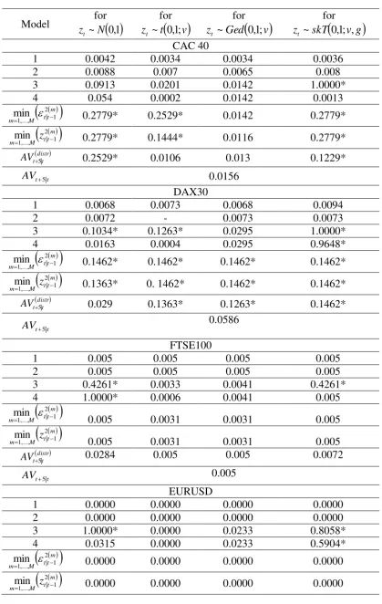
9.1.One-day-ahead Predictive Accuracy

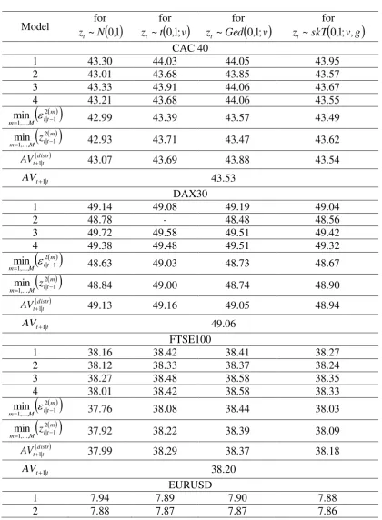
Table 4 provides the values of the mean predictive squared error, _{ } m

MPSE₁

3

10 . For

each one of the stock indices and the exchange rates, the first four rows provide the

  m

MPSE₁

3

15 (sixth) row presents the MPSE_{ }₁distr statistics from combining the forecasts of the four models

under the same distribution according to the criterion

 

 m

t t M m

2 1 | ,..., 1

min_   (

 

tt m

M

m z

2 1 | ,..., 1

min_  ). The seventh

row presents the distr t t

AV_1| statistics resulting from averaging the forecasts of the four models

under the same distribution, whereas the last row provides the overall averaging forecast,

t t

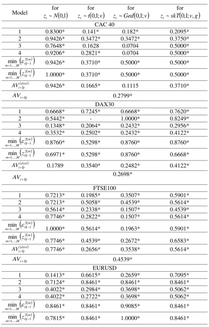
AV_1| . The relative p-values of the MCS test are presented in Table 5. For each of the

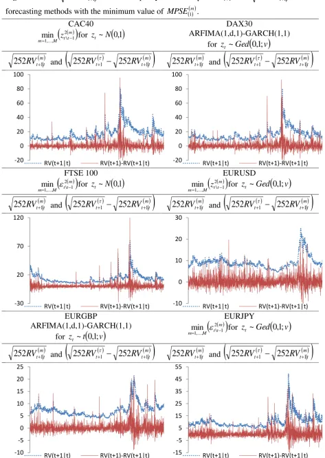
realized volatility series, Figure 2 plots the

252

RV

t m1|t and the discrepancy between

 

1

252RVt and

 m t t

RV

_1|

252

_ for the forecast methods with the minimum value of _{ } m

MPSE₁ .

Overall, we cannot infer in favor of a specific method of constructing one-day-ahead realized

volatility forecasts. The p-values in Table 5 conclude that most of the prediction methods

(single models, combined forecasts and averaged models) belong to the confidence set of the

best performing models. The lowest value of the _{ } m

MPSE₁ statistic is achieved by a single

model, the ARFIMA(1,d,1)-GARCH(1,1), in the case of the DAX30 and the Euro/Pound

rate, whereas one of the combined methods has the lowest _{ } m

MPSE₁ value for the other four

indices.

[Insert Table 4 about here]

[Insert Table 5 about here]

[Insert Figure 2 About here]

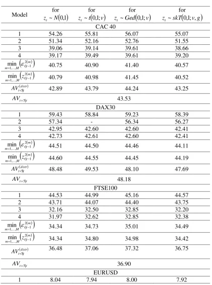
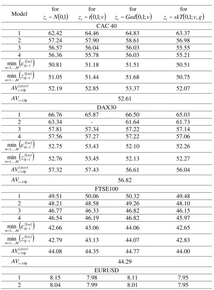
9.2.Five-days-ahead Predictive Accuracy

Table 6 shows the mean predictive squared forecast error, or MPSE  5m 3

10 for the

five-trading-days-ahead realized volatility forecasts. According to Table 7, which presents the

MCS p-values, the picture is clearer in the case of one-calendar-week-ahead forecasting. A

limited number of prediction methods belong to the confidence set of the best performing

models. Specifically, for the DAX30 index, just one model, the HAR-RV-GARCH(1,1)-skT,

belongs to the set of confidence models (for a 20% level of significance). A similar case

holds for the Euro/Pound rate, with the same model under the normal distribution

(HAR-RV-GARCH(1,1)-n) constructing the most accurate volatility forecasts. For the FTSE100 stock

index and the Euro/Dollar exchange rate, the MCS is comprised of three models, all of which

have a heterogeneous autoregressive form. In general, for five-trading-days volatility

forecasting, the heterogeneous autoregressive model is superior to the long memory

16 superior volatility forecasts for the one-calendar-week-ahead forecasting horizon (only for the

CAC40 index and the Euro/Yen rate, the

 

 m

t t M m

2 1 | ,..., 1

min_   or

 

tt m

M

m z

2 1 | ,..., 1

min_  methods of combined

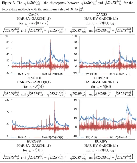
forecasts belong to the MCS). Figure 3 plots the

252

RV

t m5|t , and the forecast error

   



m



t t

t

RV

RV

₅

252

_5|

252

_



_ for the predictive methods with the minimum _{ } m

MPSE₅ .

[Insert Table 6 about here]

[Insert Table 7 about here]

[Insert Figure 3 About here]

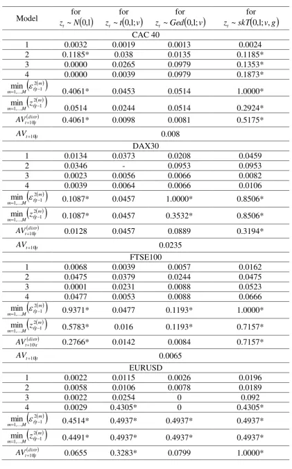
9.3.Ten-days-ahead Predictive Accuracy

Tables 8 and 9 illustrate the relative information for the two-calendar-weeks-ahead

forecasts. Overall, in the ten-days-ahead forecasting horizon, the necessity for employing

combined forecasts and averaged models arises. According to Table 9, for all the realized

volatility series under investigation the combined forecasts according to the

 

 m

t t M m

2 1 | ,..., 1

min _

  and

 

 

m

t t M

m z

2 1 | ,..., 1

min _

 criteria belong to the confidence set of the best performing methods of

forecasting. Moreover, the estimation of the models with skewed Student t distributed

standardized residuals is crucial in providing superior realized volatility forecasts. The

financial literature has delivered strong evidence in favor of modeling the asymmetric and

leptokurtic character of the log-returns distribution (see for example Degiannakis et al.,

2014). For multiple-steps-ahead forecasting, the asymmetric character of realized volatility

must be considered as well. From the different behavior of the leptokurtic distributions

(Student t and GED) and the asymmetric and leptokurtic one (the skewed Student t), we

observe that the modeling of volatility asymmetry is important for longer forecasting

horizons. For each of the six realized volatility series, Figure 4 plots the

252

RV

t m10|t , and

the discrepancy between

252

RV

t 10 and

 m t t

RV

_10|

252

_ for the forecast methods with the

minimum value of _{ } m

MPSE₁₀ .

[Insert Table 8 about here]

[Insert Table 9 about here]

[Insert Figure 4 About here]

For purposes of robustness, we have investigated the forecasting performance based on

17 report the Tables with the values of the evaluation function and the relevant MCS p-values,

which are available to the readers upon request.

10.Conclusion

Our major task is to investigate whether we can enhance our realized volatility

forecasts. The forecasting evaluation is conducted for one-day-ahead,

one-calendar-week-ahead and two-calendar-weeks-one-calendar-week-ahead horizons. The ARFIMA-GARCH and

HAR-RV-GARCH models are estimated for the major European Union stock market indices

(FTSE100, DAX30, CAC40) and for the exchange rates of the Euro with the British Pound,

the US Dollar and the Japanese Yen under the assumption that the standardized innovations

are i) normally; ii) Student t; ii) GED; and iv) skewed Student t distributed. Additionally, we

explore whether the use of a single model can be improved upon through the implementation

of a method that combines forecasts or by the averaging of the forecasts.

The overall findings can be summarized as follows. For one-day-ahead volatility

forecasts, most prediction methods (single models, combined forecasts and averaged models)

belong to the confidence set of the best performing models. For five-trading-days-ahead

forecasting horizon, the heterogeneous autoregressive model is superior to the long-memory

framework model. Moreover, the combined forecasts and the averaged models fail to provide

superior volatility forecasts. For the ten-trading-days-ahead forecasting horizon, the  

 

m

t t M m

2 1 | ,..., 1

min_   and

 

tt m

M

m z

2 1 | ,..., 1

min_  criteria deliver the most accurate volatility forecasts. Also, the

averaged models provide superior forecasts compared to those of single models.

Additionally, the modeling of volatility asymmetry (the use of the skewed Student t

distribution) is important for the ten-days-ahead volatility forecasts.

Thus, for longer forecasting horizons, more complicated forecasting frameworks are

required. Combined forecasts and averaged models are methods considered to be adequate

for volatility forecasting purposes; a crucial finding for investors, portfolio managers, risk

managers, policy makers, etc.

Avenues for future research may include the enrichment of the methods under

comparison (i.e. weights anti-proportional to the forecasting errors) or the confirmation of the

findings for other datasets, i.e. commodities, non-European stock indices, etc. It would also

be interesting to explore whether we can enhance the forecasting accuracy for other measures

of volatility, such as the realized kernels and bi-power variation, or from information

18 Acknowledgements

The author acknowledges the support from the European Community’s Seventh

Framework Programme (Marie Curie FP7-PEOPLE-IEF & FP7-PEOPLE-RG) funded under

grant agreements no. PIEF-GA-2009-237022 & PERG08-GA-2010-276904. The author is

solely responsible for any remaining errors and deficiencies.

References

Alquist, R. & Kilian, L. (2010). What do we learn from the price of crude oil futures?

Journal of Applied Econometrics, 25(4), 539-573.

Amendola, A. & Storti G. (2008). A GMM procedure for combining volatility forecasts.

Computational Statistics and Data Analysis, 52(6), 3047–3060.

Andersen, T. G., Bollerslev, T., Diebold, F. X. & Labys, P. (2003). Modeling and

forecasting realized volatility. Econometrica, 71(2), 579–625.

Andersen, T., Bollerslev, T., Christoffersen, P. & Diebold, F.X. (2006). Volatility and

Correlation Forecasting. In Elliott, G. Granger, C.W.J. and Timmermann, A. (Eds.)

Handbook of Economic Forecasting, North Holland Press, Amsterdam.

Andersen, T., Bollerslev, T. & Diebold, F. (2007). Roughing it up: including jump

components in the measurement, modelling and forecasting of return volatility. Review of

Economics and Statistics, 89(4), 701–720.

Baillie, R.T., Bollerslev, T. & Mikkelsen, H.O. (1996). Fractionally Integrated Generalized

Autoregressive Conditional Heteroskedasticity. Journal of Econometrics, 74, 3-30.

Bates, J., & Granger, C.W.J. (1969). The Combination of Forecasts. Operations Research

Quarterly, 20, 451-468.

Blair, B.J., Poon, S-H & Taylor S.J. (2001).Forecasting S&P100 Volatility: The

Incremental Information Content of Implied Volatilities and High-Frequency Index

Returns. Journal of Econometrics, 105, 5-26.

Box, G.E.P. & Tiao, G.C. (1973). Bayesian Inference in Statistical Analysis (Vol.40).

Addison-Wesley, Reading.

Chen, X. & E. Ghysels (2011). News-good or bad-and its impact on volatility forecasts over

multiple horizons. Review of Financial Studies, 24, 46–81.

Chiriac, R. & Voev, V. (2011). Modelling and Forecasting Multivariate Realized Volatility.

Journal of Econometrics, 26(6), 922-947.

Christensen, B.J., & Prabhala, N.R. (1998).The relation between implied and realised

19

Clark, T.E., & West, K.D. (2007). Approximately normal tests for equal predictive accuracy

in nested models. Journal of Econometrics, 138, 291–311.

Clements, M. P., Galvão, A. B., & Kim, J. H. (2008). Quantile forecasts of daily exchange rate returns from forecasts of realized volatility. Journal of Empirical Finance, 15(4),

729-750.

Corsi, F. (2009). A Simple Approximate Long-Memory Model of Realized Volatility.

Journal of Financial Econometrics, 7(2), 174-196.

Corsi, F. & Reno, R. (2012). Discrete-time volatility forecasting with persistent

leverageeffect and the link with continuous-time volatility modeling. Journal of

Businessand Economic Statistics, 30(3), 368-380.

Corsi, F., Mittnik, S. Pigorsch, C. & Pigorsch, U. (2008). The Volatility of Realised

Volatility. Econometric Reviews, 27(1-3), 46-78.

Degiannakis, S. (2004). Volatility Forecasting: Evidence from a Fractional Integrated

Asymmetric Power ARCH Skewed-t Model. Applied Financial Economics, 14,

1333-1342.

Degiannakis, S. (2008). Forecasting VIX. Journal of Money, Investment and Banking, 4,

5-19.

Degiannakis, S. & Xekalaki, E. (2005). Predictability and Model Selection in the Context of

ARCH Models. Journal of Applied Stochastic Models in Business and Industry, 21, 55-82.

Degiannakis, S. & Floros, C. (2015). Modelling and Forecasting High Frequency Financial

Data, Palgrave - MacMillan Ltd., Hampshire.

Degiannakis, S. & Livada, A. (2016). Evaluation of Realized Volatility Predictions from

Models with Leptokurtically and Asymmetrically Distributed Forecast Errors. Journal of

Applied Statistics, 43(5), 871-892.

Degiannakis, S. & Filis, G. (2017). Forecasting oil price realized volatility using information

channels from other asset classes. Journal of International Money and Finance, 76, 28-49.

Degiannakis, S., Floros, C. & Dent, P. (2014). A Monte Carlo Simulation Approach to

Forecasting Multi-period Value-at-Risk and Expected Shortfall Using the FIGARCH-skT

Specification. The Manchester School, 82(1), 71-102.

Deo, R., Hurvich, C. & Lu, Y. (2005). Forecasting realized volatility using a long-memory

stochastic volatility model: Estimation, prediction and seasonal adjustment. Journal of

Econometrics, 131, 29–58

Diebold, F. X., & Mariano, R. S. (1995). Comparing predictive accuracy. Journal of

20

Fernandez, C. & Steel, M. (1998). On Bayesian Modeling of Fat Tails and Skewness.

Journal of the American Statistical Association, 93, 359-371.

Fleming, J. (1998). The quality of market volatility forecast implied by S&P 100 index

option prices. Journal of Empirical Finance, 5, 317– 345.

Fleming, J., Ostdiek, B. & Whaley, R.E. (1995). Predicting Stock Market Volatility: A

New Measure. Journal of Futures Markets, 15, 265-302.

Frijns, B., Tallau, C., & Tourani‐Rad, A. (2010). The information content of implied

volatility: Evidence from Australia. Journal of Futures Markets, 30(2), 134-155.

Ghysels, E., Sinko, A., & Valkanov, R. (2007). MIDAS regressions: Further results and

new directions. Econometric Reviews, 26(1), 53-90.

Giot, P. (2003).The information content of implied volatility in agricultural commodity

markets. Journal of Futures Markets, 23, 441–454.

Giot, P. & Laurent, S. (2003). Value-at-Risk for Long and Short Trading Positions. Journal

of Applied Econometrics, 18, 641-664.

Granger, C.W.J. (1980). Long Memory Relationships and the Aggregation of Dynamic

Models. Journal of Econometrics, 14, 227-238.

Granger, C.W.J. & Newbold, P. (1977). Forecasting Economic Time Series. Academic

Press, New York.

Granger, C.W.J. & Joyeux, R. (1980). An Introduction to Long Memory Time Series

Models and Fractional Differencing. Journal of Time Series Analysis, 1, 15-39.

Granger, C.W.J. & Ramanathan, R. (1984). Improved methods of combining forecasts.

Journal of Forecasting, 3(2), 197-204.

Hansen, P.R., (2005). A test for superior predictive ability. Journal of Business and

Economic Statistics. 23, 365–380.

Hansen, P.R. & Lunde, A. (2005). A Realized Variance for the Whole Day Based on

Intermittent High-Frequency Data. Journal of Financial Econometrics, 3(4), 525-554.

Hansen, P.R. & Lunde, A. (2006). Realized Variance and Market Microstructure Noise.

Journal of Business and Economic Statistics, 24(2), 127-161.

Hansen, P.R., Lunde, A. & Nason, J.M. (2011). The model confidence set. Econometrica,

79, 456–497.

Hu, M.Y. & Tsoukalas, C. (1999). Combining conditional volatility forecasts using neural

networks: an application to the EMS exchange rates. Journal of International Financial

21

Hua, J. & Manzan, S. (2013). Forecasting the return distribution using high-frequency

volatility measures. Journal of Banking and Finance, 37(11), 4381-4403.

International Monetary Fund (2007).World Economic Outlook. Washington, DC.

Johnson, N.L., Kotz, S. & Balakrishnan, N. (1995). Continuous Univariate Distributions,

(Vol. 2) 2nd edition, John Wiley and Sons, New York.

Koopman, S. J., Jungbacker, B. & Hol, E. (2005). Forecasting daily variability of the S&P

100 stock index using historical, realised and implied volatility measurements. Journal of

Empirical Finance, 12, 445–475.

Krishnamoorthy, A.S. & Parthasarathy, M. (1951). A Multivariate Gamma - Type

Distribution. Annals of Mathematical Statistics, 22(4), 549-557.

Lambert, P. & Laurent, S. (2001). Modeling Financial Time Series Using GARCH-Type

Models and a Skewed Student Density.Universite de Liege, Mimeo.

Liu, C. & Maheu, J.M., (2009). Forecasting realized volatility: a Bayesian model‐averaging

approach. Journal of Applied Econometrics, 24(5), 709-733.

Martens, M. & Zein, J. (2002). Predicting financial volatility: High-frequency time-series

forecasts vis-`a-vis implied volatility. Journal of Futures Markets, 24(11), 1005–1028.

Müller, U.A., Dacorogna, M.M., Davé, R.D., Olsen, R.B., Pictet, O.V. &

VonWeizsäcker, J.E. (1997). Volatilities of Different Time Resolutions – Analyzing the

Dynamics of Market Components. Journal of Empirical Finance, 4, 213-239.

Patton, A.J., (2011). Volatility forecast comparison using imperfect volatility proxies.

Journal of Econometrics, 160(1), 246-256.

Pong, S., Shackleton, M. B., Taylor, S. J. & Xu, X. (2004). Forecasting currency volatility:

A comparison of implied volatilities and AR(FI)MA models. Journal of Banking and

Finance, 28(10), 2541-2563.

Prokopczuk, M., Symeonidis, L., & Wese Simen, C. (2015). Do Jumps Matter for

Volatility Forecasting? Evidence from Energy Markets. Journal of Futures Markets, 1-35.

Schwarz, G. (1978). Estimating the Dimension of a Model. Annals of Statistics, 6, 461-464.

Sévi, B. (2014). Forecasting the volatility of crude oil futures using intraday data. European Journal of Operational Research, 235(3), 643-659.

Shephard N, & Sheppard, K. (2010). Realising the future: forecasting with high frequency

based volatility(HEAVY) models. Journal of Applied Econometrics, 25, 197–231.

Svensson LEO (2005). Oil prices and ECB monetary policy.Department of Economics,

22

Wang, Y., Ma, F., Wei, Y. & Wu, C., (2016). Forecasting realized volatility in a changing

world: A dynamic model averaging approach. Journal of Banking and Finance, 64,

136-149.

Wasserfallen, W. & Zimmermann, H. (1985). The behavior of intra-daily exchange rates.

Journal of Banking and Finance, 9, 55-72.

White, H. (2000). A Reality Check for Data Snooping.Econometrica, 68, 1097–1126.

Xekalaki, E. & Degiannakis, S. (2005). Evaluating Volatility Forecasts in Option Pricing in

the Context of a Simulated Options Market. Computational Statistics and Data Analysis,

49(2), 611-629.

Xekalaki, E. & Degiannakis, S. (2010). ARCH Models for Financial Applications, John

23

[image:24.595.64.565.113.260.2]

Tables

Table 1. Information for the intra-day data.

Index

Number of intra-day (1 minute) observations

Number of trading

days

First day Last day

Optimal sampling frequency, sf o

CAC 40 1,403,509 2,708 13th June 2000 12th January 2011 7minutes

DAX 30 1,433,751 2,806 3rd January 2000 12th January 2011 13minutes

FTSE100 1,576,347 3,128 20th August 1998 12th January 2011 7minutes

EURUSD 4,622,271 3,330 20th April 1998 24th January 2011 20minutes

EURGBP 4,302,166 3,113 4th January 1999 21st January 2011 20minutes

EURJPY 4,399,091 3,131 4th January 1999 24th January 2011 20minutes

Table 2. Descriptive statistics of annualized one-trading-day inter-day adjusted realized daily

volatility, 252RVt  .

Index Mean1 Median1 Maximum1 Minimum1 Std.Dev1 Skewness Kurtosis

CAC 40 20.6 17.8 148.1 4.1 12.5 2.5 14.6

DAX 30 20.4 17.0 136.2 3.3 13.3 2.6 14.3

FTSE100 15.4 13.3 166.9 2.9 10.2 3.5 29.7

EURUSD 10.2 9.5 67.5 1.8 4.4 2.2 16.0

EURGBP 8.2 7.5 41.1 2.4 3.6 2.2 13.1

EURJPY 11.9 10.2 74.2 2.6 6.7 2.6 14.5

1

The numbers are expressed in percentages.

Table 3. Descriptive statistics of annualized inter-day adjusted logarithmic realized

volatility, log 252RVt  .

Index Mean Median Maximum Minimum Std.Dev Skewness Kurtosis

CAC 40 2.88 2.88 5.00 1.40 0.52 0.27 3.01

DAX 30 2.85 2.83 4.91 1.18 0.55 0.34 3.16

FTSE100 2.58 2.59 5.12 1.05 0.54 0.29 3.18

EURUSD 2.25 2.25 4.21 0.56 0.39 0.13 3.65

EURGBP 2.02 2.01 3.72 0.86 0.39 0.37 3.37

[image:24.595.60.512.500.601.2]

24

Table 4. The mean predictive squared error _{ } m

MPSE₁

3

10 , of the four models for

conditionally i) normally; ii) Student t

;

ii) GED

;

and iv) skewed Student t distributed innovations. The MPSE 1distri) from combining the forecasts of the four

models under the same distribution according to the criteria

 

 m

t t M m 2 1 | ,..., 1

min_   and

 

 

m

t t M m z 2 1 | ,..., 1 min _

 ; ii) from averaging the forecasts of the four models under the same

distribution ( distr t t

AV_1| ); and iii) of the overall averaging forecast (AV_t1|t).

Model _{z ~}for_N

 

_0,1

t

for



v



t z_t ~ 0,1;

for



v

