Joint Forecast Combination of Macroeconomic Aggregates and Their Components

Munich Personal RePEc Archive

Joint Forecast Combination of

Macroeconomic Aggregates and Their

Components

Cobb, Marcus P A

February 2017

Online at

https://mpra.ub.uni-muenchen.de/76556/

Joint Forecast Combination of Macroeconomic

Aggregates and Their Components

Marcus P. A. Cobb

∗

February 2017

Abstract

This paper presents a framework that extends forecast combination to include

an aggregate and its components in the same process. This is done with the ob-jective of increasing aggregate forecasting accuracy by using relevant disaggregate

information and increasing disaggregate forecasting accuracy by providing a bind-ing context for the component’s forecasts. The method relies on acknowledgbind-ing

that underlying a composite index is a well defined structure and its outcome is a fully consistent forecasting scenario. This is particularly relevant for people that are

interested in certain components or that have to provide support for a particular aggregate assessment. In an empirical application with GDP data from France,

Ger-many and the United Kingdom we find that the outcome of the combination method shows equal aggregate accuracy to that of equivalent traditional combination

meth-ods and a disaggregate accuracy similar or better to that of the best single models.

Keywords: Bottom-up forecasting; Forecast combination; Hierarchical forecasting; Reconciling forecasts

JEL codes: C53, E27, E37

Non-technical Summary

Macroeconomic forecasts receive considerable attention due to the fact that different agents

regularly use them in their decision making processes. In many situations the focus of attention is a particular aggregate and in others a whole set of them. This is the case at policy making

institutions where understanding the dynamics underlying an aggregate forecast is important to formulate useful economic policies. In such a situation some level of disaggregation may be

required.

The need for consistent forecasting scenarios means that institutions producing short-term

fore-casts usually rely on the bottom-up approach, that is building the aggregate forecast as the sum of its component’s forecasts. The bottom-up approach however is criticized because it

gener-ally cannot approximate the underlying true process and therefore may end up being inferior in terms of aggregate forecasting accuracy than alternative methods. In this context, there is an

ongoing debate on whether it is best to forecast an aggregate directly, indirectly as the sum of its component’s forecasts or in a way that uses both.

The considerable effort that has been put into improving aggregate accuracy contrasts with the apparent lack of interest in disaggregate accuracy. There is some literature that devotes itself

to exploiting the interdependence between components to increase their accuracy but hardly any that tries to take advantage of the benefits of forecasting an aggregate directly. The only

exception we find is that of Hyndman et al. (2011) that propose a method that uses individual forecasts for all levels of aggregation and optimally reconciles them so that the outcome is a

fully consistent set of forecasts. Their reconciliation method however focuses on the aggregation structure and does not take the actual forecasts into consideration.

In this paper we present a framework that benefits from both the direct and bottom-up ap-proaches to increase overall forecasting accuracy. We do so by extending the well proven and

robust results from the forecast combination literature to a setting that includes one level of disaggregation. We produce individual forecasts for the aggregate and all the components and

consider them as initial guesses. Then we update them based on their relative reliability so that they comply with the identities that define the aggregate. The problem is set in a general

con-strained quadratic program but under fairly mild assumptions derive analytical solutions making the method very easy to apply.

Our empirical application uses GDP data from France, Germany and the United Kingdom. We

find that the outcome of our method results in equal aggregate accuracy to that of equivalent

traditional combination methods and a disaggregate accuracy similar or better than that of the

best single models. Our results suggest that our framework successfully replicates the benefits

of traditional forecast combination in terms of aggregate accuracy while increasing disaggregate

1

Introduction

Assessing the state of the economy and providing an outlook for where it is heading in-volves interpreting large amounts of data in a way that is coherent. Macroeconomic

aggregates are fundamental to this process given that they synthesise the informa-tion from countless indicators into relatively few figures. Consequently, many different people and institutions devote considerable resources to predicting key economic

vari-ables. The Survey of Professional Forecasters published by the European Central Bank (ECB, 2015)1serves just as an example of this.

There are many ways in which economic variables can be forecasted and when it comes to aggregates there is also the question on whether to use the disaggregate data. In this context, one line of research has centred on determining whether forecasting an

aggregate as the sum of the forecasted components is better in terms of aggregate ac-curacy than forecasting the aggregate directly. The result of this debate, as it stands, is that it depends on the problem at hand. This view is supported by the contrasting results

from many empirical comparisons2 and the fact that for most feasible implementations which is better depends on the particular structure of the disaggregate process and the

aggregation matrix (Lütkepohl, 1987).

In some applications, however, focusing solely on the aggregate is not sufficient. As Espasa and Mayo-Burgos (2013) point out, sometimes the dynamics of the components

underlying the aggregate forecast are of as much interest as the aggregate itself. It is often the case that practitioners rely on methods in which the aggregate is produced as

the sum of the forecasts of its components because they have to be able to explain what underlies an aggregate forecast (Esteves, 2013; Ravazzolo and Vahey, 2014). In such cases a direct approach is not a viable option.

There are strong arguments however in favour of using direct approaches when the con-cern is aggregate accuracy. Granger (1987) show that common factors that are relat-ively unimportant at an individual level may dominate the aggregate while Hendry and

Hubrich (2011) argue that, given that the bottom-up strategy is usually implemented by forecasting the disaggregate components independently from each other, it cannot

properly approximate the underlying multivariate process. In this context, a forecaster

1

The ECB Survey of Professional Forecasters collects expectations on inflation, real GDP growth and unemployment in the euro area from experts affiliated with financial and non-financial institutions from within the area (Garcia, 2003).

2_{For example Espasa et al. (2002), Benalal et al. (2004), Hubrich (2005) and Giannone et al. (2014) for}

that is concerned with overall accuracy would want to benefit from the direct methods if possible.

One strategy could be simply to use direct methods for the aggregate and reconcile the disaggregate forecasts. This would not take into consideration however that theoret-ical and empirtheoret-ical results suggest that both the direct and bottom-up approaches are

valuable. It would be very appealing therefore to be able to benefit from both.

If the concern were only for the aggregate, a popular way of dealing with two competing forecasts would be simply to combine them. The idea of forecast combination was put

forward quite a while ago in Bates and Granger (1969) and deals with the issue of ex-ploiting in the best possible way the information contained in each individual forecasts. The literature on it is extensive and the surveys by Clemen (1989), Diebold and Lopez

(1996), Newbold and Harvey (2002) and Timmermann (2006) not only give testimony of it but also highlight the robustness of the gains in forecasting accuracy due to its use.3

Notwithstanding the extensive literature on combination methods, almost all of it deals

with one variable at a time. A notable exception is that of Hyndman et al. (2011). They propose a method that uses individual forecasts for all levels of aggregation and

optimally reconciles them so that the outcome is a fully consistent set of forecasts. A striking feature of their implementation is that the combination weights depend only on the aggregation structure and not on the forecasts themselves. This apparently

counter-intuitive result stems directly from a key assumption. This is that the forecast errors follow the same aggregation pattern as the data.

In this paper we present a framework that extends the notions developed in the

combin-ation literature to a setting that includes one level of disaggregcombin-ation but where it is not necessary to make any assumptions regarding the forecast errors. To this effect, we

ap-proach the combination process from a slightly different perspective to that of Hyndman et al. (2011). Similarly to them, we produce individual forecasts for the aggregate and all the components and consider them as initial guesses. We then however update them

based on their relative reliability so that they comply with the identities that define the aggregate.

On the one hand, our framework has the potential of increasing aggregate forecasting

accuracy if relevant disaggregate information is not picked up by traditional (aggregate) combination methods. On the other hand it has the potential of increasing disaggregate forecasting accuracy by providing a binding context for the individual forecasts. The

3_{Timmermann (2006) summarize a number of rationales that make combining forecasts appealing, most}

gains from constraining disaggregate forecasts, at least in regards to the aggregate, are supported theoretically by Giacomini and Granger (2004).

The rest of the paper is organized as follows. Section 2 develops the framework that allows for the combination of series from two different levels of aggregation. Section 3 presents an empirical implementation using GDP data for France, Germany and the

United Kingdom. Section 4 summarizes the conclusions.

2

Combining Forecasts from Different Aggregation Levels

People working on the compilation of aggregate statistics regularly face the need to bal-ance information from different sources in order to produce official statistics. In many of those applications, like the production of national accounts and the social-accounting

matrices, the reconciliation process involves a massive amount of data meaning that throughout the years automatic procedures have been proposed to iron out the

differ-ences.4

In a recent paper, Rodrigues (2014) cast the whole problem of balancing statistical eco-nomic data into a Bayesian framework. They suggest treating the data as stochastic

processes, modelling their prior properties accordingly and finding the balanced pos-terior by means of relative entropy minimization.

The process proposed by Rodrigues (2014) equates to searching for a posterior

distri-bution that is as close as possible to the prior that satisfies the required restrictions. Although their implementation is specific to balancing economic data, the principle

be-hind their framework resembles the problem of any sort of forecast combination. The individual forecasts serve as best guesses, different forecasts have different reliability and cross-sectional identities must be met. They establish that a number of the

con-ventional reconciliation methods are in fact particular cases of their general framework and show that there is a one-to-one correspondence. Based on this correspondence,

they argue that it is possible to identify the conventional method’s underlying assump-tions and go on to suggest using least squares approaches when uncertainty estimates are available.

4_{Most of the methods can roughly be classified either as constrained optimization methods or as}

2.1

A Constrained Optimization Forecast Combination Framework

The problem is approached as that of finding the forecasts that are as close as possible to the preliminary figures that satisfy the required restrictions. In particular we focus on

a least-squares squares formulation that translates into letting the undefined criterion for as close as possible to be governed by some quadratic loss function. We concentrate on solving the problem for one level of disaggregation, that is an aggregate and its

components, as it is a setting that is relevant for many practical applications.

2.1.1 Formulating the Problem

The problem may be expressed as a general constrained quadratic program of the form:

min

α,β A

X

i=1

f

i,t

(

y

i,t

, α

i,t

, ϕ

i,t

)

2

+

D

X

d=1 N

X

n=1

g

d,n,t

(

q

d,n,t

, β

d,n,t

, φ

d,n,t

)

2 (1)

subject to:

(1 +

α

1,t

)

y

1,t

−

N

X

n=1

(1 +

β

1,n,t

)

w

1,n,t

q

1,n,t

= 0

(1 +

α

1,t

)

y

1,t

−

(1 +

α

i,t

)

y

i,t

= 0

for

i

= 2

to

A

(1 +

β

1,n,t

)

q

1,n,t

−

(1 +

β

d,n,t

)

q

d,n,t

= 0

for

d

= 2

to

D

,

n

= 1

to

N

where

y

i,t is the preliminary forecast for time

t

of the

i

-th aggregate model of a total

of

A

,

α

i,t is the percentage deviation of the definitive forecast from the preliminary,

ϕ

i,t

is its exogenously chosen optimization weight and

f

i,t is some function of the three.

Similarly,

q

d,n,tis the preliminary forecast for time

t

for component

n

of the

d

-th model

of a total of

D

disaggregate models,

β

d,n,t is the percentage deviation of the definitive

forecast from the preliminary,

φ

d,n,tis its exogenously chosen optimization weight,

g

d,n,t

is some function of the three and

w

d,n,tis the respective aggregation weight.5

The accounting identities are reflected directly in the constraints, but determining an appropriate loss function for the minimization problem is not straightforward. The

liter-ature on forecast combination is of little help because it has not dealt with the issue of combining different levels of aggregation in this way.6 The reconciliation literature on the other hand has several suggestions, but given that they have been developed for a

5_{It is worth mentioning that all variables are in levels and that for simplicity it is assumed that all}

components and aggregation weights are strictly positive.

6

different purpose it is necessary to make sure that they are adequate for the combina-tion context.

We proceed by finding a loss function that in a setting where using a traditional

single-variable forecasting combination method is feasible it produces the same outcome. In particular, we concentrate on the equal-weighted average due to its robust performance.

The following two assumptions provide the foundations for a setting where this method may be used:

1. The reliability of all forecasts are known to be the same.

2. All the information relevant for forecasting contained in the components is

trans-mitted to the aggregate level.

These assumptions make working with the components equivalent to only dealing with their sum. In this context, the solution for this basic setting, using the nomenclature of

equation (1), is:

˜

y

t

=

1

A

+

D

A

X

i=1

y

i,t

+

D

X

d=1 N

X

n=1

w

d,n,t

q

d,n,t

!

(2)

Although this setting could be seen as unrealistic, simple combination schemes are used extensively and there is ample evidence that in practice they often perform better than more involved procedures (Timmermann, 2006). In fact, the relative performance and

robustness of the equal-weighted forecast combination is such that it has raised interest among researcher to try to explain it and has come to be known as the forecast

combin-ation puzzle (Smith and Wallis, 2009).

2.1.2 A Joint Combination Method for a Single Set of Forecasts

In developing a method that combines aggregate and disaggregate forecasts we start by focusing only on one set of forecasts. That is, for some period

t

, for a composite

index

X

that is constructed by summing

N

components

x

n using the respective

time-varying aggregation weights

w

n, there is a direct forecast

y

t and a set of forecasts

for its components

q

n,t. In this context, two popular approaches that come from the

reconciliation literature are the proportional and additive distribution methods. The proportional approach penalizes percentage deviations from the preliminary forecasts

which translates into the loss function:

ϕ

t

h

(1+αt)yt−yt

yt

i

2

+

P

N_n=1

φ

n,t

h

_(1+β

n,t)qn,t−qn,t

qn,t

i

2

=

ϕ

t

α

2t

+

P

N

Assigning discrepancies proportionally means bigger components absorb a larger share of the total adjustment. On the contrary, the additive approach attempts to evenly

spread out the discrepancies among the variables. The associated loss function is:

ϕ

t

[(1 +

α

t

)

y

t

−

y

t

]

2

+

P

N_n=1

φ

n,t

[(1 +

β

n,t

)

q

n,t

−

q

n,t

]

2

=

ϕ

t

(

α

t

y

t

)

2

+

P

N_n=1

φ

n,t

(

β

n,t

q

n,t

)

2

(4)

Unfortunately, both approaches applied directly fail to arrive at the desired outcome. On the one hand, the solution from a proportional approach is invariable strictly lower

than the simple average of the aggregate forecasts. On the other hand, once aggregate and components are included into the same problem the outcome from the additive approach presents a bias towards the preliminary aggregate forecast. Although neither

of the approaches produce the desired results when applied directly, it is possible to develop an appropriate loss function by recovering their respective desirable features.7

We start from equation (4) but impose a larger penalty term on the components so as to

eliminate the aforementioned bias. Doing this results in the loss function being:

ϕ

t

(

α

t

y

t

)

2

+

Q

t N

X

n=1

φ

n,t

w

n,t

q

n,t

β

n,t2 (5)

with

Q

t

=

P

N_n=1

(

w

n,t

q

n,t

)

.

Using this loss function and minimizing it subject to

(1 +

α

t

)

y

t

−

P

N_n=1

w

n,t

(1 +

β

n,t

)

q

n,t

gives as a solution that the definitive aggregate forecast for

X

tis:8

˜

y

t

= ˜

Q

t

=

Q

2 t

+

y

t

N

X

n=1

ϕt

φn,t

w

n,t

q

n,t

Q

t

+

N

X

n=1

ϕt

φn,t

w

n,t

q

n,t

(6)

and the definitive forecast for the component

x

n,tis:

˜

q

n,t

=





1 +

ϕ

t

φ

n,t

·

y

t

−

Q

t

Q

t

+

P

N_n=1

ϕt

φn,t

w

n,t

q

n,t





q

n,t (7)

For the case of equal reliability, that is making

ϕ

i,t and

φ

d,n,t equal to one, it becomes

7

All this is shown in detail in section A.1 of the Appendix.

clear that equation (6) becomes a simple average. That is:

˜

y

t

=

Q

2

t

+

y

t

Q

t

2

Q

t

=

Q

t

+

y

t

2

(8)

2.1.3 A Joint Combination Method for Multiple Sets of Forecasts

For one set of forecasts the loss function suggested in the previous section results in the desired outcome. If more than one set of forecasts is considered for each variable

however the outcome of the equal reliability case is not equal to the simple average.9 Fortunately the bias that appears can be avoided simply by combining the multiple fore-casts for the individual series before performing the joint combination and choosing the

optimization weights so as to reflect the prior step.

Let the result for the prior step be:

y

t

=

1

Γ

t

A

X

i=1

γ

i,t

y

i,t and

q

n,t

=

1

∆

n,t

D

X

d=1

δ

d,n,t

q

d,n,t (9)

with

γ

i,t and

δ

d,n,t being the reliability weights,

Γ

t

=

P

_i=1A

γ

i,t and

∆

n,t

=

P

D_d=1

δ

d,n,t.

The joint combination procedure remains unchanged except for the weights

ϕ

tand

φ

n,t

that are set to reflect the reliability of the combined forecasts

y

t and

q

n,tas opposed to

the initial preliminary forecasts

y

i,t and

q

d,n,t.

In the case of equal reliability, this means accounting for the fact that the problem as

a whole involves

A

aggregate and

D

disaggregate forecasts. That is accomplished by setting

ϕ

t

=

A

and

φ

n,t

=

D

making the solution for the aggregate forecast:

˜

y

t

=

1

A

+

D

A

·

y

t

+

D

·

N

X

n=1

w

n,t

q

n,t

!

(10)

By expanding the individual forecasts, given that

γ

i,t and

δ

d,n,t are equal to one, the

definitive aggregate forecast is left in terms of the preliminary estimates:

˜

y

t

=

_A+D1

A

·

_A1

P

A_i=1

y

i,t

+

D

·

P

N_{n=1 D}1

w

n,t

P

D_d=1

q

d,n,t

=

_A+D1

P

A_i=1

y

i,t

+

P

D_d=1

P

N_n=1

w

n,t

q

d,n,t

(11)

that is the same as taking the simple average of all the available forecasts for the

ag-gregate.

9

This result shows that the method replicates the outcome of the equal-weighted forecast combination for the aggregate while at the same time providing component forecasts

that are fully consistent. More generally however, the framework admits taking into consideration the reliability of the different forecasts.10 This is a desirable feature when the uncertainty surrounding the different forecast differs like, for example, in the case of nowcasting where necessary inputs may include both preliminary and definitive figures.

2.1.4 Feasible Region for the Reliability Weights

From the solution in equation (6) we notice that what matters is the relative reliability and that therefore any given number in isolation is meaningless. It is important however

to establish a feasible region that provides a unique solution for the minimization prob-lem. We do this by looking at the bounds for the weights and what they imply regarding

overall reliability. Considering as a starting point that all weights are set equal to one:

1. Absolute Certainty: The limit for a high degree of reliability is to eliminate all uncertainty from the outcome. For the aggregate forecast this means making

ϕ

t

go to infinity. In such a case it is easy to see that

lim

ϕt→∞

(1 +

α

t

)

y

t

=

y

t. On

the other hand, for a single component

n

= 1

, setting

ϕ

t back to one and making

φ

1,t go to infinity implies that φϕ1t,t

→

0

. This means that the weight given to the

direct forecast decreases but still remains positive. Taking it to the extreme and

making all component’s weights go to infinity decreases the weight given to the direct forecast to zero. That is

lim

φt→∞

(1 +

α

t

)

y

t

=

Q

twhere

φ

n,t

=

φ

tfor

n

= 1

to

N

. All forecasts however cannot be certain otherwise the problem does not have a solution. This means the ceiling for reliability weights is infinity but at least one of them has to be finite.

2. Zero Confidence: The opposite to a high degree of reliability is to have absolutely no confidence whatsoever in a forecast. For the aggregate forecast this would mean making

ϕ

t

= 0

and therefore

y

˜

t

=

Q

t. On the converse, for a single

compon-ent

n

= 1

, setting

ϕ

t back to one and making

φ

1,t

= 0

means that this component

absorbs all the deviation. This is clear from appreciating that ϕt

φ1,t

→ ∞

and

there-fore that

lim

φ1,t→0

(1 +

α

t

)

y

t

=

y

t. This basically means that the forecasts from all

but this component are taken as given and that the definitive forecast

q

˜

1,tis found

residually. It is worth noting that this can be done for one variable only otherwise

the minimization problem has infinite solutions. This means that no more than one variable can have a reliability weight equal to zero for the problem to have a unique solution.

10_{For this case in which only one level of disaggregation is considered it is easy to show that the method}

For the purpose of allowing for some degree of combination it makes sense to restrict the aggregate forecasts to have finite reliability weights. This means that a given

com-ponent could have a weight that implies certainty, maybe due to the early release of relevant data, but not all of them.

3

Combining GDP Forecasts for Three European Economies

As an empirical application of the method we perform a forecasting exercise using GDP data from France, Germany and the United Kingdom. We use eight different

forecast-ing models and four different ways of establishforecast-ing the combination weights within our framework. We evaluate the aggregate forecasting accuracy by comparing the results

with that of the single models and traditional forecast combinations. The forecasting accuracy of the components is evaluated against that of the single-models.

3.1

Data

For the exercise we use GDP series from both the production and expenditure ap-proaches for France, Germany and the United Kingdom. The data is quarterly and seasonally adjusted, spanning from 1991 to 2014 and available from the OECD

statist-ics database.11

As in most of the OECD, these countries calculate their GDP using a chain-linking method.12 _{A well known rather unpleasant feature of this method is that the volume} of changes in inventories cannot be constructed as chain-linked series (Lequiller and Blades, 2014). This is problematic because they are required in order to complete the

aggregate GDP forecasts from the expenditure approach.

Faced with this problem, some authors proceed by expressing the series in terms of con-tributions to GDP growth and adjust their methods accordingly. In order to avoid dealing

with a series that becomes close to zero and changes sign often we bundle change in inventories with imports. The rational behind that is that in practice changes in

invent-ories to a great extent serve as a buffer for foreign trade and considering them together could be beneficial. This is supported by Esteves (2013) who find that forecasting errors

11

For the United Kingdom the production data on the OECD database starts in 1995. The first four years of the sample are obtained by splicing backwards the historical reference tables available from the Office for National Statistics. No inconsistencies arise from the seasonal adjustment given that the aggregates are adjusted indirectly, that is as the sum of the seasonally adjusted components.

12

of imports and changes in inventories are highly correlated and that forecasting them jointly increases forecasting accuracy.

Taking all that into consideration, the breakdown of aggregate GDP for all three coun-tries is the following:

Table 1: GDP Production and Expenditure Components

Production:

1. Agriculture, forestry and fishing 7. Financial and insurance activities 2. Manufacturing 8. Real estate activities

3. Industry and energy, excluding manufacturing 9. Professional, administrative and support service activities 4. Construction 10. Public adm., defence, social security, education and health 5. Trade, transport, accommodation and food services 11. Other service activities

6. Information and communication 12. Taxes less subsidies Expenditure:

1. Private consumption 4. Exports of goods and services

2. Government expenditure 5. Imports of goods and services and changes in inv. 3. Gross fixed capital formation

3.2

Forecasting Models

Regardless of the numerous developments in econometric modelling, univariate meth-ods continue to provide an often strong benchmark against which to compare other models (Marcellino, 2008). They are also the methods used in many of the

aggregate-disaggregate forecasting competitions mentioned in the literature review and are there-fore a reasonable starting point.

For this purpose we use a random walk for the growth rate, an autoregressive model of

order one for the first differences of the variables and ARIMA models chosen following a common and well established routine. In particular we rely on the program TRAMO

(Gomez and Maravall, 1996) that through an automatic procedure selects the appropri-ate transformation and chooses the model based on the Bayesian Information Criterion (BIC).

To account for the interdependence between components we also use Bayesian Vector Autoregressive models (BVARs) following the implementation in Banbura et al. (2010). In particular, the two first sets of VARs include the Consumer Price Index (CPI) and the

respective approach, that is: only the aggregate GDP, only the production side compon-ents and only the expenditure componcompon-ents, estimated with all variables in first

differ-ences and also differentiating CPI twice.

Following the notion in Hendry and Hubrich (2011) we also estimate VARs that include all the GDP variables and CPI in the same model. We cast the VARs in levels, first

The smallest VARs, that is the two that include CPI and only the aggregate GDP, are estimated by OLS using two lags. All the others are estimated using five lags and the

choice of overall tightness, as in Banbura et al. (2010), is made such that the in-sample fit equals that of a two-variable VAR with five lags estimated by OLS over the first 10

years of the sample.

All this results in eight sets of forecasts over the forecasting horizon for each one of the

variables.

3.3

Forecasting Accuracy Comparison

3.3.1 Set-up of the Evaluation Exercise

The evaluation exercise is performed over the 2001-2014 period leaving the first years of data to estimate the models. It is set up in a quarterly rolling scheme using a ten

year window where in each period the models are re-estimated and a one-year-ahead quarterly forecast is generated.

The forecasting accuracy is presented, for different horizons, by means of the model’s

mean square forecasting error (MSFE) relative to that of a benchmark model. That is, for variable

i

, horizon

h

and using model

m

, the relative MSFE is

RelMSFE

(i,h,m)

=

MSFE

(i,h,m) T0,T1

MSFE

(i,h,0)_T0,T1

with

MSFE

(i,h,m)_T0,T1

=

1

T

1

−

T

0

+ 1

T1

X

t=T0

y

(m)_i,t+h

|

t

−

y

i,t+h

2

where

y

_i,t+h(m)

|

t

is the forecasted value for

t

+

h

at time

t

and

T

0is the last period of actual

data in the first sample used for the evaluation and

T

1is the last period of actual data in

the last sample. As usual a RelMSFE lower than one reflects an improvement over the

benchmark model for which

m

= 0

.

Regarding measuring the overall forecasting accuracy of the components we do so by comparing the cumulative absolute errors in the contribution to the aggregate level.

For this purpose we define the cumulative absolute root mean square forecasting error for an aggregate with

N

components

q

n, horizon

h

and using model

m

as

CumRMSFE

(h,m)_T0,T1

=

v

u

u

u

t

1

T

1

−

T

0

+ 1

T1

X

t=T0 N

X

n=1

w

n,t+h

·

abs

q

(m)_n,t+h

|

t

−

q

n,t+h

where

q

_n,t+h(m)

|

t

is the forecasted value for

t

+

h

at time

t

and

T

0 is the last period of actual

data in the first sample used for the evaluation and

T

1is the last period of actual data in

the last sample.

3.3.2 Specific Forecast Combination Minimization Problem

The empirical exercise contemplates combining forecasts for GDP from direct approaches and disaggregate approaches from the production and expenditure sides.

Let the result of the prior combination step be a unique direct forecast

y

, a production side forecast

Q

based on the

N

components

q

nand an expenditure side forecast

G

based

on the

M

components

g

m. Then, the minimization problem involving the aggregate

reliability weight

ϕ

, the production reliability weights

φ

n, the expenditure reliability

weights

ψ

m, the production aggregation weights

w

n and the expenditure aggregation

weights

ω

m, is:

min

α,β,ǫ

ϕ

t

(

α

t

y

t

)

2

+

Q

t N

X

n=1

φ

n,t

w

n,t

q

n,t

(

β

n,t

)

2

+

G

t M

X

m=1

ψ

m,t

ω

m,t

g

m,t

(

ǫ

m,t

)

2 (12)

subject to:

(1 +

α

t

)

y

t

−

P

_n=1N

w

n,t

(1 +

β

n,t

)

q

n,t

= 0

(1 +

α

t

)

y

t

−

P

_m=1M

ω

m,t

(1 +

ǫ

m,t

)

g

m,t

= 0

Similarly to the simple setting, this problem also has analytical solutions.13 The definit-ive aggregate forecast also follows a weighted average form:

˜

y

t

=

Υ

t

·

y

t

+ Ω

t

·

Q

t

+ Ξ

t

·

G

t

Υ

t

+ Ω

t

+ Ξ

t

(13)

where

Υ

t

=

P

N_n=1

ϕt

φn,t

w

n,t

q

n,t

·

P

M_m=1

ϕt

ψm,t

ω

m,t

g

m,t

,

Ω

t

=

Q

t

·

P

_m=1M _ψϕ_m,tt

ω

m,t

g

m,t and

Ξ

t

=

G

t

·

P

N_n=1φϕ_n,tt

w

n,t

q

n,t. The definitive forecasts for all of the components can in turn

then be easily recovered using a solution similar to that of equation (7).

3.3.3 Establishing Reliability Weights

Even in the absence of relevant external knowledge it may be desirable to determine reliability weights based on the properties of the preliminary estimates. Timmermann

(2006) present an extensive survey on some of the suggestions from the combination lit-erature for single variables and more become available from ongoing research (Hansen,

2008; Wei and Yang, 2012; Hsiao and Wan, 2014).

Taking into consideration the easiness with which each suggestion can be incorporated into our framework we choose a few.

Equal Weights:

An obvious choice for the first set of weights is equal weights because it serves as the benchmark against which to compare all the others.

In-Sample Fit:

Using in-sample fit to determine combination weights is not uncommon. Kapetanios

et al. (2008) find promising results from using weights calculated using information criteria. Extending this approach to compare different series is not straightforward. We can however extend the way that Banbura et al. (2010) determine in-sample fit for their

Bayesian VARs by normalizing the measure.

We start by defining the root mean square percentage error (RMSPE) at time

u

using information up to time

p

for the

h

-step ahead forecast of

x

i as:

RM SP E

i,u,p,h,v

=

v

u

u

t

1

v

u−h

X

s=u−h−v

x

i,s+h

|

p

x

i,s+h

−

1

2

(14)

where

x

i,s+h

|

p

is the fitted value for

x

i using the coefficients calculated at time

p

and

v

determines how much data is included in the measure. The latter is limited by the number of lags that are included in each model.

We then define the weights based on in-sample fit as:14

ω

ISP_i,t,h,v

=

1

RM SP E

i,t,t,h,v

(15)

Out-of-Sample Past Performance:

An obvious extension of the idea of weighting according to predictability is to weigh the different forecasts based on their recent past relative out-of-sample performance. This

approach goes as far back as Bates and Granger (1969). Empirical studies suggest that

14

In the context of forecast combination using predictive measures, Eklund and Karlsson (2007) raise awareness regarding the possibility of distorting weight distribution due to overconfidence in models that over-fit data. Aiolfi and Favero (2005) for example use the model’sR2 _{to decide on the combination of}

forecasts weighted by the inverse of their MSE are found to work well in practice (Stock and Watson, 1999; Timmermann, 2006).

Following the same idea and arguments expressed for the in-sample fit weights, we define the weights based on out-of-sample past performance as:

ω

_i,t,h,vOSP

=

1

RM SP E

i,t,s,h,v

(16)

where in this case the

s

that goes into the formula as the time subscript is not a para-meter, but the index in the sum embedded in equation (14).

Optimal weights:

In the context of single variable combinations Granger and Ramanathan (1984) address the problem of determining the optimal combination weights as a least-squares

regres-sion problem. Hyndman et al. (2011) extend the approach to a setting with variables from different aggregation levels. In their implementation however they do not consider forecasts from more than one hierarchical order. To enable combining forecasts from

both the production and expenditure approaches we use an approximation and set the weights to:15

ω

OPT

i,t

=

x

i,t

P

N n=1

x

i,t

(17)

In the case of all weighting methods the reliability weights are calculated for every

rolling window. For the in-sample the five most recent years of the window are used and for the out-of-sample weights the last two.

3.3.4 Aggregation weights

Before being able to perform the forecasting exercise one final point needs to be ad-dressed. Given the chain-linked nature of the series, the aggregation weights required

for the forecasting process are not fixed. This is a relevant issue as Lütkepohl (2011) and Brüggemann and Lütkepohl (2013) show that accounting for the changing weights

can increase forecasting accuracy significantly.

In the chain-linking framework aggregation weights depend on previous year prices and therefore for short forecasting horizons some information regarding the prices that will

go into the weights is available. To take this issue into consideration without having to actually forecast the aggregation weights, we use a simple adaptive procedure to

[image:18.595.82.513.127.305.2]

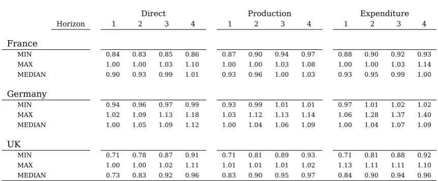
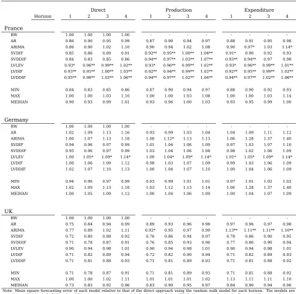
Table 2: Single Model Aggregate Relative Forecasting Errors by Approach

Direct Production Expenditure Horizon 1 2 3 4 1 2 3 4 1 2 3 4

France

MIN 0.84 0.83 0.85 0.86 0.87 0.90 0.94 0.97 0.88 0.90 0.92 0.93 MAX 1.00 1.00 1.03 1.10 1.00 1.00 1.03 1.08 1.00 1.00 1.03 1.14 MEDIAN 0.90 0.93 0.99 1.01 0.93 0.96 1.00 1.03 0.93 0.95 0.99 1.00

Germany

MIN 0.94 0.96 0.97 0.99 0.93 0.99 1.01 1.01 0.97 1.01 1.02 1.02 MAX 1.02 1.09 1.13 1.18 1.03 1.12 1.13 1.14 1.06 1.28 1.37 1.40 MEDIAN 1.00 1.05 1.09 1.12 1.00 1.04 1.06 1.09 1.00 1.04 1.07 1.09

UK

MIN 0.71 0.78 0.87 0.91 0.71 0.81 0.89 0.93 0.71 0.81 0.88 0.92 MAX 1.00 1.00 1.02 1.11 1.01 1.01 1.01 1.02 1.13 1.11 1.11 1.10 MEDIAN 0.73 0.83 0.92 0.96 0.83 0.90 0.95 0.97 0.84 0.90 0.94 0.96

Note: Minimum, median and maximum of the mean square forecasting error of the individual models relative to that of the direct approach using the random walk model for each horizon. The individual models are a random walk with drift, a first-differences autoregressive model of order one, an ARIMA chosen according to the Bayesian Information Criterion, two small VARs including CPI and the GDP variables from each approach in first differences and where CPI is differenced twice and three large VARs including CPI and all GDP variables in levels, in first differences and in first differences with CPI differenced twice. Calculated for one to four steps ahead forecasts over the 2001-2014 period.

provide estimates of the unavailable weights. This procedure consists on using the implicit deflator that results from the most recent four-quarter moving averages of the non-seasonally adjusted nominal and chain-linked series to have an updated estimate of

the future aggregation weights.16

3.4

Results

3.4.1 Forecast Combination Accuracy Over the Whole Sample

The forecasting application involves eight different forecasting models and three

differ-ent approaches. Table 2 presdiffer-ents the minimum, median and maximum of the individual models’ relative forecasting accuracy for the aggregate over the 2001-2014 sample for the three countries.17

Looking at the differences between countries it becomes apparent that for France and the UK there are quite significant improvements over the naive random walk model while in the case of Germany most models do worse. For all three countries however

the direct approach tends to achieve the best results.

16

According to the survey in OECD (2009) updated to April 2015, almost 72% of the OECD members and the OECD itself use the annual overlap method for their quarterly accounts and therefore we use this method for this exercise. It should be noted that the United Kingdom uses the slightly different quarterly overlap method.

17

[image:19.595.133.462.128.330.2]

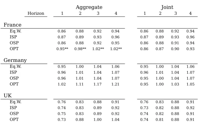
Table 3: Combination Aggregate Relative Forecasting Error

Aggregate Joint

Horizon 1 2 3 4 1 2 3 4

France

Eq.W. 0.86 0.88 0.92 0.94 0.86 0.88 0.92 0.94

ISP 0.87 0.89 0.93 0.96 0.87 0.89 0.93 0.96

OSP 0.86 0.88 0.92 0.95 0.86 0.88 0.91 0.94

OPT 0.95** 0.98** 1.02** 1.02** 0.86 0.87 0.90 0.93

Germany

Eq.W. 0.95 1.00 1.04 1.06 0.95 1.00 1.04 1.06

ISP 0.96 1.01 1.04 1.07 0.96 1.01 1.04 1.07

OSP 0.96 1.01 1.04 1.07 0.95 1.00 1.04 1.07

OPT 1.02 1.11 1.17 1.21 0.95 1.00 1.03 1.05

UK

Eq.W. 0.76 0.83 0.88 0.91 0.76 0.83 0.88 0.91

ISP 0.74 0.83 0.89 0.92 0.73 0.82 0.88 0.92

OSP 0.75 0.83 0.89 0.92 0.74 0.82 0.88 0.91

OPT 0.73 0.88 1.00 1.04 0.74 0.81 0.88 0.91

Note: Mean square forecasting error of each model relative to that of the direct approach using the random walk model for each horizon. The combination weighting schemes are the simple average (EQ.W), in-sample fit (ISP), out-of-sample performance (OSP) and optimal weights (OPT). For the aggregate optimal weightswe use the approach in Conflitti et al. (2015) that impose the constraints that weights should be non-negative and sum up to one.* and ** denote that the respective forecast is statistically worse than the best single model within the sample according to the Modified Diebold-Mariano statistic at a 10 and 5% significance level. Calculated over the 2001-2014 period.

The overall dispersion in forecasting accuracy between single models varies among

countries.18 For France the comparison between the minimums achieved for each ho-rizon with the maximums show that the worst performing models are between 20 and

30% less accurate depending on the horizon while the same comparison for the me-dian show differences of 10 to 20%. For Germany the same comparison shows that the worst performing models are between 10 and 20% less accurate while for the median

differences are around of 10%. For the UK the differences are between 20 and 40% and around 10% respectively.

Given the varying performance of the models it could turn out to be quite costly choos-ing one only. The appeal of forecast combination is that this is not necessary and Table 3 presents their RelMSFE for this exercise. In the column under the “Aggregate”

head-ing we present the outcome for the traditional forecast combination for shead-ingle variables applied to the aggregates that result from all three approaches calculated using equi-valent weighting schemes.19 _{In the column under the “Joint” heading we present the} outcome of our framework.

The first thing to notice is that overall the differences between weighting schemes are

very small within each approach. The only exception is the aggregate optimal combin-ation. The second is that there is hardly no difference between the aggregate accuracy

18

The outstandingly bad ARIMA for expenditure approach is removed for the analysis of maximums.

19

[image:20.595.126.477.268.584.2]

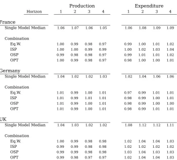
Table 4: Cumulative Disaggregate Relative Forecasting Error

Production Expenditure

Horizon 1 2 3 4 1 2 3 4

France

Single Model Median 1.06 1.07 1.06 1.05 1.06 1.08 1.09 1.09

Combination

Eq.W. 1.00 0.99 0.98 0.97 0.99 1.00 1.01 1.02

ISP 1.00 1.00 0.99 0.99 1.00 1.02 1.03 1.04

OSP 0.99 0.98 0.98 0.97 0.99 1.01 1.01 1.02

OPT 1.00 0.99 0.98 0.97 0.98 1.00 1.00 1.01

Germany

Single Model Median 1.04 1.02 1.02 1.03 1.02 1.04 1.06 1.06

Combination

Eq.W. 1.01 0.99 1.00 1.01 0.97 0.99 1.01 1.01

ISP 1.01 0.99 1.01 1.01 0.98 0.99 1.00 1.01

OSP 1.01 0.99 1.00 1.01 0.98 0.99 1.00 1.00

OPT 1.01 0.99 1.00 1.01 0.98 0.99 1.01 1.01

UK

Single Model Median 1.04 1.03 1.02 1.02 1.08 1.12 1.12 1.11

Combination

Eq.W. 1.00 0.99 0.98 0.98 1.02 1.04 1.04 1.03

ISP 0.99 0.99 0.98 0.98 1.02 1.02 1.02 1.02

OSP 0.99 0.99 0.98 0.98 1.03 1.04 1.03 1.03

OPT 0.99 0.98 0.97 0.97 1.02 1.04 1.04 1.03

of the joint combination and its traditional counterpart. This means that no harm in this sense is caused by using our framework. In fact, for the UK the joint

combin-ation performs marginally better for most weighting schemes. Regarding the actual performance, as one would expect given that all models enter with positive weights, the

minimum RelMSFE from the single models are not achieved. They do however come well below the median of the single models.

In regards to the disaggregate accuracy, Table 4 presents the CumRMSFE of the joint

method for both the production and expenditure approaches relative to that of the best single model within each approach for each horizon. The results show that some of the features present at the aggregate level translate to the components. In particular the

overall differences between weighting schemes are very small within each approach.

The most remarkable result however is the fact that for all three countries the joint

combination often improves on the best performing single model. In the case of France for the production approach the accuracy from most of the combination methods is at least as good as the best single model and improves up to 3%. For the expenditure

approach on the other hand it improves up to 2% but mostly equals or is up to 2% worse. With regards to the median the combinations are approximately 7% better for both production and expenditure. In the case of Germany the major improvements

are found for the expenditure approach with up to 3%. Overall for both approaches the accuracy of the combination are very similar to the best model and from 2 to 5%

better than the median. For the UK there is an overall improvement for the production approach of up to 3%. The expenditure approach on the other hand does no improve but remains quite close to the best model. Overall for both approaches the accuracy of

the combination is from 4 to 8% better than the median.

Overall we find that the joint combination methods perform well given that most of them achieve similar accuracy as the best performing single model of each approach in

a context where the best single models of each approach are not necessarily consistent with each other or as good as the combined forecast in terms of aggregate accuracy.

3.4.2 Aggregate Forecasting Accuracy Over the Evaluation Sample

One non-trivial detail of our forecasting exercise is that the evaluation period includes

the end portion of what has been called the Great Moderation and the 2008 world finan-cial crisis. A considerable body of literature has devoted itself to understand the effects of these periods on forecasting models and Chauvet and Potter (2013) present a

[image:22.595.85.507.119.474.2]

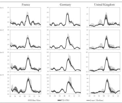
Figure 1: Dispersion of the Rolling Forecasting Error

Note: Four-quarter rolling root mean square forecasting error (RMSFE) for each horizon. The Min-Max shaded area shows the span between the minimum and maximum RMSFE from the 24 individual models/approaches in each period. The P20-P80 does the same but trims off the top and bottom 20%. joint is the median of the joint combination methods. Calculated as four-quarter moving windows over the 2001-2014 period.

stable times completely failed with the increase of volatility and that models perform dif-ferently in expansions and recessions. This last point had been previously documented

in Marcellino (2008) who find that in recessions their more sophisticated models showed a marked deterioration making the simple random walk the best performer.

For the purpose of our exercise this could lead to our results being overly influenced by the particular performance in the crisis years simply because the forecasting errors

could be massive. It makes sense therefore to look at how the forecasting errors evolve over the sample. To do so, we look at the four-quarter rolling root mean square error for all forecasting horizons. Figure 1 presents the dispersion of the single models referred

to as min-max, the same measure trimming the best and worst performing 20% and the median of the joint combinations.

as suspected, the size of the forecasting errors would make this period predominant in the overall results.

Regarding other aspects, the picture looks relatively similar across forecasting horizons within countries but a bit different for each country. For France the dispersion of the models seems relatively high before and after the financial crisis and not so much

dur-ing it and the effect of the crisis on forecastdur-ing accuracy is relatively short-lived. For Germany on the other hand dispersion is relatively low over the whole sample but the

effects of the crisis on accuracy go on for much longer than for the other two countries. For the UK the dispersion is relatively low before the crisis, but high during it and re-mains moderately high thereafter. The forecasting errors decrease really fast after the

crisis.

Regarding the performance of the combination method, the median measure registers

values at or very close to the lower boundary of the trimmed dispersion measure for most of the evaluation sample.

The way in which errors evolve over the sample suggest that the crises years could

be too determinant in the overall results. We therefore perform the previous analysis excluding years 2008 and 2009 from it. The episode and its consequences are bound to be long lasting and for this reason, although we remove its direct impact on the measure

for forecasting accuracy, the effects on the estimation of the parameters remain.

As before, Table 5 presents the relative forecasting accuracy for the aggregate of the single models but this time for the restricted sample.

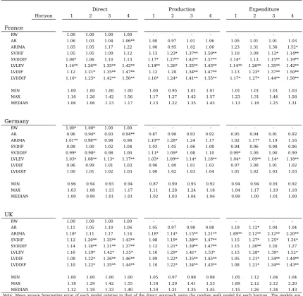
The changes are quite dramatic. For France and the UK the improvements of the models over the random walk completely disappear. In fact, most of the models turn out to be

significantly worse. Only for Germany does the general picture look similar. Also, in this case it is the bottom-up production side approach that shows marginally better results.

The significant increase in overall dispersion in forecasting accuracy between single

models for both France and the UK is clear from comparing the minimum and the me-dian. For the former it goes up to 10 to 30% depending on the horizon and the latter to 10 to 40%. For Germany on the other hand the same measurement remains around

10%.

The performance of the forecast combination however does not appear that different

[image:24.595.84.512.158.343.2]

Table 5: Single Model Forecasting Errors excluding 2008-2009

Direct Production Expenditure

Horizon 1 2 3 4 1 2 3 4 1 2 3 4

France

MIN 1.00 1.00 1.00 1.00 1.00 0.95 1.01 1.01 1.01 1.01 1.01 1.03 MAX 1.16 1.26 1.42 1.56 1.17 1.27 1.42 1.57 1.23 1.31 1.44 1.58 MEDIAN 1.06 1.06 1.13 1.17 1.13 1.22 1.35 1.45 1.13 1.18 1.25 1.31

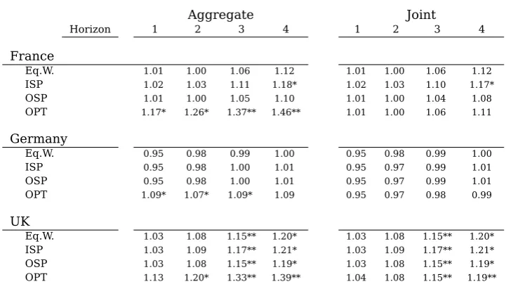
Germany

MIN 0.96 0.94 0.93 0.94 0.87 0.90 0.93 0.92 0.94 0.94 0.91 0.92 MAX 1.03 1.08 1.13 1.17 1.11 1.28 1.24 1.18 1.04 1.17 1.19 1.18 MEDIAN 1.00 0.99 1.01 1.01 1.02 1.03 1.04 1.06 0.99 1.00 1.01 1.00

UK

MIN 1.00 1.00 1.00 1.00 1.05 0.97 0.98 0.98 1.05 1.12 1.04 1.04 MAX 1.18 1.29 1.42 1.55 1.18 1.29 1.41 1.53 1.89 2.12 2.12 2.20 MEDIAN 1.12 1.19 1.33 1.40 1.10 1.21 1.35 1.45 1.15 1.26 1.34 1.43

Note: Minimum, median and maximum of the mean square forecasting error of the individual models relative to that of the direct approach using the random walk model for each horizon. The individual models are a random walk with drift, a first-differences autoregressive model of order one, an ARIMA chosen according to the Bayesian Information Criterion, two small VARs including CPI and the GDP variables from each approach in first differences and where CPI is differenced twice and three large VARs including CPI and all GDP variables in levels, in first differences and in first differences with CPI differenced twice.. Calculated for one to four steps ahead forecasts over the 2001-2014 period excluding years 2008 and 2009.

Table 6: Combination Aggregate Forecasting Error excluding 2008-2009

Aggregate Joint

Horizon 1 2 3 4 1 2 3 4

France

Eq.W. 1.01 1.00 1.06 1.12 1.01 1.00 1.06 1.12

ISP 1.02 1.03 1.11 1.18* 1.02 1.03 1.10 1.17*

OSP 1.01 1.00 1.05 1.10 1.01 1.00 1.04 1.08

OPT 1.17* 1.26* 1.37** 1.46** 1.01 1.00 1.06 1.11

Germany

Eq.W. 0.95 0.98 0.99 1.00 0.95 0.98 0.99 1.00

ISP 0.95 0.98 1.00 1.01 0.95 0.97 0.99 1.01

OSP 0.95 0.98 1.00 1.01 0.95 0.97 0.99 1.01

OPT 1.09* 1.07* 1.09* 1.09 0.95 0.97 0.98 0.99

UK

Eq.W. 1.03 1.08 1.15** 1.20* 1.03 1.08 1.15** 1.20*

ISP 1.03 1.09 1.17** 1.21* 1.03 1.09 1.17** 1.21*

OSP 1.03 1.08 1.15** 1.19* 1.03 1.08 1.15** 1.19*

OPT 1.13 1.20* 1.33** 1.39** 1.04 1.08 1.15** 1.19**

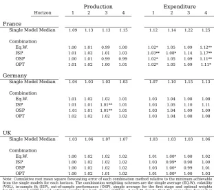
[image:24.595.117.478.472.674.2]

[image:25.595.141.453.128.405.2]

Table 7: Cumulative Disaggregate Forecasting Error excluding 2008-2009

Production Expenditure

Horizon 1 2 3 4 1 2 3 4

France

Single Model Median 1.09 1.13 1.13 1.15 1.12 1.14 1.22 1.25

Combination

Eq.W. 1.00 1.01 0.99 1.00 1.02* 1.05 1.09 1.12**

ISP 1.01 1.03 1.01 1.03 1.03** 1.08* 1.14 1.17**

OSP 1.00 1.01 0.99 0.99 1.02* 1.05 1.09 1.11**

OPT 1.01 1.02 1.00 1.01 1.02* 1.05 1.09 1.11*

Germany

Single Model Median 1.04 1.03 1.03 1.03 1.07 1.10 1.15 1.13

Combination

Eq.W. 1.01 1.02 1.02 1.01 1.03 1.04 1.08 1.08

ISP 1.01 1.01 1.01** 1.01 1.03 1.05 1.10 1.11

OSP 1.01 1.01 1.01** 1.01 1.03 1.04 1.09 1.09

OPT 1.02 1.02 1.02 1.02 1.03 1.04 1.08 1.08

UK

Single Model Median 1.03 1.06 1.07 1.07 1.03 1.03 1.03 1.06

Combination

Eq.W. 1.00 1.02 1.02 1.02 1.01 1.00* 1.00 1.02

ISP 1.00 1.02 1.02 1.02 1.03 0.99* 0.98 1.00

OSP 1.00 1.02 1.02 1.02 1.03 1.00* 0.99 1.01

OPT 1.00 1.02 1.01 1.02 1.01 1.00* 1.00 1.03

Note: Cumulative root mean square forecasting error of each combination method relative to the minimum achievable from the single models for each horizon. The combination weighting schemes are the simple average (EQ.W), volatility (VOL), in-sample fit (ISP), out-of-sample performance (OSP), simple average for the first stage and optimal weights for the second (OPT-1) and optimal weights for both stages (OPT-2). * and ** denote that the respective forecast is statistically worse than the best single model within the sample according to the Modified Diebold-Mariano statistic at a 10 and 5% significance level. Calculated over the 2001-2014 period excluding years 2008 and 2009.

its traditional counterpart with some joint combination methods performing marginally better.

Regarding the actual performance however the RelMSFE of the combinations are

fur-ther from that of the best single models. For France they are between 1 and 10% worse but still 15% better than the median model. For Germany they are about 9% worse and between 2 and 5% better than the median. For the UK they are between 5 and 20%

worse and between 10 and 15% better than the median. Also, the performance of the combination methods deteriorates for the longer horizons.

In regards to the disaggregate accuracy, Table 7 presents the cumulative RMSFE of the joint method for both the production and expenditure approaches relative to that of the best single model within each approach for each horizon.

In this case the overall differences between weighting schemes are again very small within each approach. It is noteworthy however that, notwithstanding the increased dispersion in performance that results from removing the crisis from the sample, some

The overall performance looks quite good. In the case of France for the production approach the accuracy from most of the combination methods is very similar to that of

the best single model. This is not achieved for the expenditure approach however that is up to 10% worse. Nevertheless, with regards to the median the combinations are

approximately 10 to 15% better for both production and expenditure. Similarly, in the case of Germany the accuracy is similar for the production approach but suffers for the expenditure approach and exhibits a similar improvement over the median to that of

the whole sample. For the UK both for production and expenditure the combinations perform similarly to the best model and up to 5% better than the median.

3.4.3 Comments on the Overall Results.

In general terms the results suggest that there are benefits from using forecast com-bination in this particular case and that most of the gains of doing so are picked up by

the equal-weighted scheme. In particular the alternative weighting schemes provide only marginally different results both for the aggregate and the joint combination

ap-proaches. Nevertheless the possibility of introducing external knowledge into the com-bination procedure provides flexibility to the forecaster.

The fact that the aggregate accuracy of the joint combination methods is practically the

same, and in some cases marginally better, to that of the equivalent traditional method suggests that the benefits of achieving disaggregate consistency do not come at the cost of the aggregate accuracy.

In fact, given that the combination methods show disaggregate forecasting accuracy similar or better to those of the best performing single models suggests that the

con-straints that they impose do in fact transmit the benefits of the aggregate methods to the components.

Finding relatively comparable results for three different countries and isolating the

dir-ect effdir-ect of the financial crisis provides some robustness to the method. This suggests that this method could serve as a valid alternative to the bottom-up only approach.

4

Conclusion

relying on the merits of the individual forecasts and acknowledges that for any real-ized outcome an aggregate is exactly the weighted sum of its components. This method

makes use of disaggregate components and ensures that the accounting identities that underlie the aggregate are met delivering a completely consistent forecasting scenario.

An important feature of our framework is that it imposes no constraints on the way

inn which the forecasts that enter the combination framework are made. Any forecast, based on a model or not, may be used. Given that the method guarantees a

consist-ent scenario, the strengths of the direct aggregate forecast may be transferred to the component’s forecasts by effectively constraining the disaggregate set as a whole. This means that some degree of interdependence is forced on the component’s forecasts no

matter if they are generated independently or not in the first place.

In our empirical application with GDP data from France, Germany and the United King-dom, we find that our combination framework provides equal aggregate forecasting

accuracy to that of equivalent traditional forecast combination methods and disaggreg-ate accuracy similar or better to those of the best performing single models. All this

suggests this method is a valid alternative to bottom-up only approaches when a fully consistent scenario is required.

Our method shares many common features with that of Hyndman et al. (2011) but

ex-tends it in two aspects. First, it makes it possible to use in contexts where there are multiple forecasts for each variable and multiple distinct possible disaggregations. For example the three different approaches for GDP. Second, it allows to use weights that

reflect the relative reliability of the preliminary forecasts themselves. Although in our empirical application the reliability weights determined from the data did not make much of a difference when compared to equal weights, the posibility of establishing the

weights coul prove to be useful as a way of introducing external information or judge-ment into the forecasting process. This is something that Central Banks do regularly as

a way of incorporating a broader assessment of relevant conditions that are not expli-citly accounted for in their models (Alessi et al., 2014).

A logical step for further research would be to extend our framework to admit multiple

levels of disaggregation as is the case with Hyndman et al. (2011). Another immediate area is to explore using it for density forecasting in order to see how it affects the whole distribution. From an applied perspective it would be interesting to enrich the set of

models that are included in the combination process. Some obvious candidates would be to add factor models that have boosted the performance of direct aggregate forecasts

Appendix

A

Empirical Framework

A.1

Joint Combination with Equal Reliability

Let there be a composite index

X

that results from the simple sum of

N

≥

2

strictly positive components

x

n. Let there be two forecasts for

X

for period

t

. The first,

y

t,

comes from forecasting

X

directly, while the second one,

Q

t, is the simple sum of the

forecasts of its components

q

n,t.

A.1.1 Optimization Weights for One Set of Forecasts

The proportional deviation approach from the reconciliation literature finds the definit-ive value for

X

by making the differences between it and the initial estimates propor-tional. The minimization problem is therefore:

min

α,β

(1 +

α

)

y

−

y

y

2

+

(1 +

β

)

Q

−

Q

Q

2

+ 2

λ

[(1 +

α

)

y

−

(1 +

β

)

Q

]

(18)

where

α

and

β

are the percentage deviations of the definitive value from the initial

estimates.20

The first order conditions imply that

Q

=

−

β_α

y

and

(1 +

α

)

y

=

Q

+

βQ

. The aggregate forecast resulting from solving the problem is then:

˜

y

= (1 +

α

)

y

= (1 +

β

)

Q

=

y

·

Q

y

2

+

Q

2

(

y

+

Q

)

(19)

Using the inequality of arithmetic and geometric means we have that

0

≤

(

y

−

Q

)

2

=

y

2

+

Q

2

−

2

yQ

_{. Then}

2

yQ

≤

y

2

+

Q

2 _{and therefore:}

y

·

Q

y

2

+

Q

2

≤

1

2

meaning that equation (19) is strictly lower than an equal weighted average if both forecasts are distinct.

The additive deviation approach on the other hand finds the definitive value for

X

by

making the differences between it and the initial estimates equal in absolute terms.

20

The minimization problem can be written as:

min

α,β

[(1 +

α

)

y

−

y

]

2

+ [(1 +

β

)

Q

−

Q

]

2

+ 2

λ

[(1 +

α

)

y

−

(1 +

β

)

Q

]

₍₂₀₎

The first order conditions imply that

β

=

−

α

_Qy and

(1 +

α

)

y

= (1 +

β

)

Q

. Then replacing

β

in the latter gives

(1 +

α

)

y

=

Q

−

αy

(21) and solving for

(1 +

α

)

y

you get the simple average.

The result does not hold however if the additive approach is used directly on the com-ponents forecasts. In that case, the minimization problem is the following:

min

α,βn

(

αy

)

2

+

P

N_n=1

(

β

n

q

n

)

2

+ 2

λ

h

(1 +

α

)

y

−

P

N_n=1

(1 +

β

n

)

q

n

i

(22)

This time the first order conditions imply that

β

n

=

−

α

_qy_n for

n

= 1

to

N

and

(1 +

α

)

y

=

P

N

i=1

(1 +

β

n

)

q

n. Solving for

(1 +

α

)

y

you get that the aggregate forecast resulting from

the combination is:

˜

y

=

N

·

y

+

P

N n=1

q

n

N

+ 1

=

1

N

+ 1

(

N

·

y

+

Q

)

(23)

that is different to the simple mean given that

N

≥

2

and both aggregate forecasts are assumed to be distinct.

From comparing both approaches it can be seen that the only difference between the two is that the latter eliminates the downward bias by penalizing deviations based on

the relative size of each aggregate forecast. The same idea can be extended to find the appropriate penalty term for the components.

Including an unspecified weight

η

n for the disaggregate components in equation (22)

results in:

min

α,βn

(

αy

)

2

+

N

X

n=1

(

β

n

η

n

)

2

+ 2

λ

"

(1 +

α

)

y

−

N

X

n=1

(1 +

β

n

)

q

n

#

(24)

This time the first order conditions imply that

β

n

=

−

q_ηn2

n

·

αy

for

n

= 1

to

N

and

(1 +

α

)

y

=

P

N

i=1

(1 +

β

n

)

q

n. Using this gives:

(1 +

α

)

y

=

N

X

n=1

(

q

n

)

−

N

X

n=1

q

2n

η

2 n

·

αy

Then matching with the intermediate step given by equation (21) results in:

Q

−

N

X

n=1

q

_n2

η

2 n

·

αy

Then solving for

η

nthe weight for the components is:

η

n

=

p

q

n

·

Q

With this, the loss function that produces the equal weighted result for the aggregate

is:

(

αy

)

2

+

N

X

n=1

q

n

Q

(

β

n

)

2 (25)

A.1.2 Joint Combination for Multiple Distinct Disaggregate Forecasts

The previous framework is not limited to one set of disaggregate forecasts. It can

in-corporate more forecasts providing they are distinct, that is that they are not based on the same components. To show this let there be a third forecast,

G

, that is the simple sum of the

M

forecasts of its components

g

m. Again assuming all aggregate forecasts

are equally reliable the minimization problem may be written as:

min

α,βn,γm

(

αy

)

2

+

P

N_n=1

q

n

Qβ

n2

+

P

M

m=1

g

m

Gγ

m2

+ 2

λ

1

h

(1 +

α

)

y

−

P

N_n=1

(1 +

β

n

)

q

n

i

+ 2

λ

2

h

(1 +

α

)

y

−

P

M_m=1

(1 +

γ

m

)

g

m

i

(26)

The

N

+

M

+ 3

first order conditions are:

1. _∂α∂

:

αy

+

λ

1

+

λ

2

= 0

2. _∂β∂

n

:

β

n

Q

−

λ

1

= 0

for

n

= 1

to

N

3. _∂γ∂

m

:

γ

m

G

−

λ

2

= 0

for

m

= 1

to

M

4. _∂λ∂

1

:

(1 +

α

)

y

−

P

N

i=1

(1 +

β

n

)

q

n

= 0

5. _∂λ∂₂

:

(1 +

α

)

y

−

P

M_m=1

(1 +

γ

m

)

g

m

= 0

This time the first order conditions imply th