Expansionary Austerity and Reverse Causality

Munich Personal RePEc Archive

Expansionary Austerity and Reverse

Causality

Breuer, Christian

Chemnitz University of Technology, Department of Economics,

Junior Professorship for European Economics

15 March 2017

1

Expansionary Austerity and Reverse Causality

Christian Breuer

Chemnitz University of Technology Department of Economics

Junior Professorship for European Economics [email protected]

This version: July, 20171

Abstract

We show that the cyclical adjustment strategy used in a large stream of literature on the conventional or data-based analysis of fiscal policy fails to correct for cyclical effects in the case of expenditure-GDP-ratios so that the finding of expansionary austerity in this literature is based on reverse causality, i.e. increasing GDP causally decreases expenditure-GDP-ratios and not vice versa. Proposing a new version of the

“Blanchard”-method of cyclical adjustment, correcting for this error, and replicating Alesina and Ardagna (2010), the expansionary effects of fiscal consolidations disappear or turn into opposite. These findings may help understanding some of the controversies in the recent literature and contribute to a rehabilitation of the conventional approach

and the “Blanchard method” to compute cyclically-adjusted government budget data.

Keywords: fiscal adjustment; Blanchard method; cyclical adjustment; reverse causality JEL Classifications: E 62, E 63, H 50

1 _{I thank Olivier Blanchard for helpful comments on a previous version of this paper, and Pablo}

2

1. Introduction

One of the lively debated issues in today’s macroeconomic research is the question of

the effects of fiscal policy. Since the European fiscal crisis, this debate gained political relevance because policy-makers around the world have been in search of an efficient

way to reduce government debt levels. The idea of an “expansionary fiscal contraction”

seemed to be one tempting solution for the challenges of the time.

Macroeconomic textbooks in the Keynesian tradition however suggest that fiscal expansions increase, while fiscal consolidations contract aggregate demand. A reduction of government deficit levels would thus decrease economic growth in the short run. On the other hand, a substantial amount of research on the macroeconomic effects of fiscal consolidations challenges this conventional wisdom and finds that fiscal adjustments

may have expansionary economic effects (‘expansionary austerity hypothesis’). This

view was first expressed by Giavazzi and Pagano (1990) who discussed the expansionary effects of cases of fiscal adjustments in Ireland and Denmark during the

1980s. Alesina and Perotti (1995)2 found first evidence for the expansionary austerity

hypothesis in a large panel of OECD countries. In the aftermath, a number of papers built on the approach used in A&P (1995) to investigate the effects of fiscal policy.3 According to this stream of literature, fiscal consolidations are likely to be expansionary if the adjustment mainly takes place on the expenditure side, while tax increases are

more likely to be contractionary (Alesina and Ardagna, 1998, 2010, and 2013).4

To measure discretionary changes in fiscal policy, A&P investigate changes in the

cyclically-adjusted primary balance (hereafter: conventional or data-based approach)

and apply a cyclical adjustment strategy based on the so-called “Blanchard method”

(hereafter: A&P approach).5

Critique of this approach is not new. In a comment on A&P, Kollintzas (1995) criticised that the cyclical adjustment strategy used in A&P (1995) might not capture the cyclical

effects of the government budget balance so that the resulting “Blanchard Fiscal

2 _{Hereafter A&P.}

3 _{See for instance Alesina and Perotti (1997), Alesina and Ardagna (1998, 2010, and 2013), and Ardagna}

(2004 and 2009).

4

Hereafter A&A (1998, 2010, and 2013).

5 _{The cyclical adjustment strategy is motivated by Blanchard (1990) and described by Alesina and Perotti}

3

Indicator” (BFI) might not be an appropriate measure of a discretionary change in fiscal

policy. Moreover, Giavazzi (1995) suggests that the results in A&P are influenced by accompanying monetary policies, in form of exchange rate devaluations, for example in

the case of Ireland 1987.6

At the beginning of the European fiscal crisis, there was a renewed interest in the effects of fiscal consolidations and potential expansionary effects. Against this background, A&A (2010 and 2013) provided new evidence on expansionary effects of fiscal consolidations in a panel of OECD countries. These studies have been frequently debated in the recent literature.7 Different from A&A (2010), Leigh et al. (2010) and Guajardo et al. (2014) analysed historical records of fiscal adjustments and contrasted the conventional approach with the historical approach. Their results did not share the

expansionary austerity view.

Guajardo et al. (2014) illustrate that the fiscal indicator as used in A&A (2010) is correlated with GDP forecast revisions. The authors state that estimates based on the conventional approach appear to be biased towards overestimating expansionary effects, since the conventional approach entails one-offs operations in the budget balance. They also criticise that the cyclical adjustment strategy of A&A (2010) neglects the effects of budgetary effects of changes in asset prices. Jayadev and Konczal (2010) and Jordà and Taylor (2016) illustrate that the successful cases of fiscal adjustments in A&A (2010) are in most instances associated with an economic upswing, an analysis that questions

the exogeneity of the fiscal indicator used in the data-based approach. In this line,

De-Cos and Moral-Benito (2013) illustrate that fiscal adjustment episodes as identified by A&A (2010) are not exogenous to economic growth and treat fiscal consolidations as weakly exogenous or predetermined, pointing to potential feedback effects and reverse causality. However, De-Cos and Moral-Benito (2016) illustrate that the cases of fiscal

adjustments identified by the narrative approach are not exogenous to GDP, too.

To account for potential endogeneity in the study of A&A (2010), Holden and Midthjell (2013) and Yang et al. (2015) applied alternative measures of discretionary change and illustrate that the positive effect of fiscal adjustments disappears after applying

6 _{The same critique holds for the episodes examined in Giavazzi and Pagano (1990).}

7 _{Refer to Blyth (2013) and Stiglitz (2016) for a comprehensive discussion and critique of expansionary}

4

alternative strategies of adjusting budgetary data for cyclical effects, rather than adjusting with the method used in A&A.

After the Blanchard method used in A&A (2010) has been criticised for the (non-) recognition of fluctuations in asset prices and their effect on the budget balance (Guajardo et al., 2014), Yang et al. (2015) developed an indicator of fiscal impulse which controls for asset price fluctuations and discovered that the results are more in-line with the narrative approach when the changes in the fiscal stance is measured with this alternative strategy. Very close to the study at hand, Holden and Midthjell (2013) discussed potential reverse causality in the study of A&A (2010) and illustrate that reductions in government spending are not more likely to be successful in terms of reducing government debt, compared to tax increases, if the CAPB is estimated with a modified strategy, rather than the strategy used by A&A. However, Holden and Midtjell (2013) as well as Yang et al. (2015) apply newly developed strategies to adjust for cyclical effects rather than applying standard methods of cyclical adjustments and do not show whether their assumptions are more in line with the literature, compared to the assumptions on the cyclical sensitivity of the government budget made in A&P (1995), as well as A&A (1998, 2010, and 2013). Moreover, Holden and Midthjell (2013) focus on the question of whether fiscal policies are effective in reducing debt, rather than examining the effect of the cyclical adjustment strategy on the estimated fiscal

multiplier. To this end, no previous study discussed why the Blanchard method as used

in the literature following A&P is in conflict with standard assumptions on automatic stabilizers and how fixing this conflict influences the estimated fiscal multiplier in conventional analyses of fiscal policy.

5

Section 2 of this paper illustrates that the strategy pioneered by A&P is in conflict with standard assumptions made in the literature on cyclical adjustment. Different from the assumptions proposed in the literature, A&P implicitly assume unit-elastic government expenditures with respect to GDP, while it is common to assume inelastic government expenditure (other than transfers). To fix the incomplete cyclical-adjustment problem, an augmented specification of the BFI is proposed. Section 3 summarizes the theoretical discussion and proposes testable hypotheses on how the different strategies to adjust for cyclical effects influence the estimated fiscal multiplier. The following empirical parts test these hypotheses based on the dataset used in A&A (2010) and contrast the A&P approach with a CAPB based on a standard cyclical adjustment strategy and the

augmented version of the BFI.8

Section 4 provides evidence for the hypothesis that the fiscal indicator as used in A&A (2010) entails a pro-cyclical pattern and is positively correlated with the output gap, while the same is not true for the CAPB of the OECD or the augmented version of the Blanchard method. As predicted in section 2, this pattern appears to be particularly pronounced for the expenditure-GDP-ratio (if calculated with the A&P method).

Section 5 analyzes large changes of the output gap and illustrates that episodes with large changes in the output gap are very likely to be picked as an episode of large discretionary change in A&A (2010) if the A&P method is used, rather than the CAPB, as computed by the OECD or the augmented version of the BFI.

Replicating A&A (2010) in section 6, the estimated effects are compared (based on the CAPB used in A&A, the CAPB of the OECD, and the augmented BFI. In line with the hypotheses formulated in section 3, it is shown that the results based on the A&A measure provide evidence for expansionary effects of fiscal contractions in the case of expenditure cuts, while this effect is contractionary after using standard assumptions to correct for cyclical effects. Section 7 computes dynamic effects of fiscal policy based on the three strategies to compute the CAPB. It is shown that there is a qualitative difference in the estimated fiscal multiplier if standard methods are used to compute the CAPB, rather than the method proposed by A&A. Section 8 concludes.

8 _{In the empirical part of the paper I use the same data and definitions as A&A (2010), precisely the}

6

2. Cyclical adjustment and reverse causality

2.1. Cyclical adjustment and the data-based approach

To analyse the effects of changes in fiscal policy on GDP, the conventional (data-based)

approach applies regressions of GDP growth rates y_t in year t on changes in the

cyclically-adjusted primary budget balances (as a ratio to GDP) capb_t:

(1) yt 







capbt 



t

The idea of this approach is quite straightforward: coefficient  captures the effect of a

change in fiscal policy (measured as a percentage point of GDP) on GDP growth rates, i.e, the fiscal multiplier. This approach provides unbiased estimates of the fiscal

multiplier if the CAPB_t is assumed to be unaffected by GDP growth (no reverse

causality). Because the budget balance is influenced by a number of factors (that might be correlated with the economic cycle), the question of reverse causation has often been discussed in the literature. Foremost, Perotti (2013) highlights two potential pitfalls of empirical papers on the effects of fiscal policy using the conventional approach, the

“countercyclical response problem”, and the “imperfect cyclical adjustment problem”.

Since the cyclical adjustment strategy aims at controlling for the automatic feedback effects of GDP on the budget balance, the most obvious reason why the budget balance

responds to GDP seems to be controlled for, however, an “incomplete cyclical

adjustment problem” arises when the cyclical adjustment strategy applied does not appropriately account for cyclical effects in the budget balance, f. e. because it does not take into account changes in asset prices. In this context, a number of articles discuss

the influence of asset prices on the budget balance.9 While the cyclical adjustment

strategy controls for automatic effects of GDP on the budget balance, another non-automatic effect might arise through discretionary policy measures.

9 _{See Morris and Schuknecht (2007) and Yang et al. (2015) on how asset price fluctuations might}

7

For example, it is possible that systematic counter-cyclical policy responses might contribute to the positive relationship between the budget balance and economic growth

(“counter-cyclical response problem”). Accordingly, the estimated coefficient  is an

unbiased assessment of the fiscal multiplier only under the assumption of no “imperfect

cyclical adjustment problem” and no “counter-cyclical response problem”. In the

following, we focus on the incomplete cyclical-adjustment problem in the literature using the conventional approach and the Blanchard-method to adjust for cyclical effects in the tradition of A&P (1995).

2.2. The Blanchard method in the tradition of A&P

Typical cyclical adjustment strategies (as for instances applied in the OECD economic outlook) aims at controlling for automatic feedback from changes in the economic cycle

to the budget balance using an estimated budget sensitivity (to the output gap) g:

(2) CAPBt PBt 



gGapt

Here, Gap represents the output gap (as a percentage of potential GDP), where potential

GDP is to be measured with a production function or filtering methods, what is a potential source of measurement error. Since a number of authors have been skeptical regarding the reliability of estimations of potential output and thus the output gap, Blanchard (1990) suggests using the unemployment rate as a natural indicator of the

economic cycle rather than estimates of the output gap10:

(3) CAPBt PBt 



uURt

A&P (1995) pioneered data-based analyses and the so-called “Blanchard method” to

adjust the budget balance for cyclical effects with estimations of u. They refer to the

so computed change in the fiscal stance as the “Blanchard fiscal indicator” (equation 3).

10 _{According to Blanchard (1990) an estimation of the level of potential GDP is not necessary anyway,}

8

The basic question in the article at hand is how to measure the budget sensitivity (with

respect to unemployment) u, and whether and how the cyclically adjustment strategy

proposed in A&P is in line with the assumptions made in the literature on cyclical adjustment, particularly whether there are potential pitfalls at the spending- or revenue side. Fedelino et al. (2009) is referred to as a benchmark study on cyclical adjustment, even though there are other pioneering discussions of cyclical adjustment strategies, for example Girouard and André (2005). According to Fedelino et al. (2009), the CAPB consists of cyclically-adjusted revenues net of cyclically-adjusted expenditure, both

adjusted with their respective sensitivity to GDP (here, P

t

Y represents potential GDP)11:

(4) G R t P t t P t t t Y Y G Y Y R CAPB                    

The literature on cyclical adjustment proposes the following simplifying assumptions:

unit-elastic revenues (responding to the tax base with an elasticity of 1),



_R = 1, and

inelastic government expenditure (



G = 0). If so, equation (4) can be simplified to

(5) t

t P t t t G Y Y R

CAPB _

      

To adjust the budget balance for cyclical effects, it appears to be reasonable to adjust revenues but not expenditure. However, since some expenditure items - as in the case of unemployment benefits - are affected by the economic cycles, it might be necessary to take into account elastic transfer payments (because unemployment benefits increase in an economic downturn). Following this line, Alesina and Perotti (1995) assume that social transfers to households, as well as revenues (and only transfers and revenues) respond to cyclical effects. Consequently, A&P apply the cyclical adjustment procedure to taxes and transfers, whereas expenditures other than transfers remain unadjusted.

9

According to A&P12 and equivalent to equation (3), the BFI is

(6) CAPBt Rt 



RURt (Trt 



TrURt)Gt

Rather than computing estimates of potential GDP and output elasticities, here it is necessary to compute estimates of the elasticities of transfers and tax revenues with

respect to unemployment (_R and



_Tr).

To do so, for each country A&P regress social transfers as a share of GDP13 on two time

trends (one for the full period and one for the period after 1975 to control for a potential

structural break)14 and on the unemployment rate:

(7) Tr_t a₀a₁trend₁a₂trend₇₅



_Tr UR_t e_t

Then A&P estimate what the transfers would be in period t if unemployment rates were the same as in the previous year:

(8) Tr_t UR_t a a trend a trend _Tr UR_t et

  

 



1) 0 1 1 2 75  1

(



Here, 0



a , 1



a , 2



a , and



Tr

 represent estimated coefficients (and e is the residual) of

equation (7). The difference between unemployment-adjusted transfers Trt(URt_1)

according to equation (8) and previous’ years’ transfers Trt1 is regarded as a measure

of the change in cyclically-adjusted transfers (equivalent to equation 6).

(9) CATrt Trt  TrURt





The elasticity of transfers with respect to unemployment _Tr is estimated with equation

(7). The same procedure is applied for revenues to achieve unemployment-adjusted

12 _{This definition remains relatively similar to the follow up papers, as e. g. in A&A (1998, 2010, 2013).} 13 _{Note that in A&P the fiscal variables are expressed as ratios to GDP.}

10

revenues (Rt(URt_1) ). With the construction of Trt(URt1) and Rt(URt1), A&P

estimate the primary deficit that would have prevailed in period t if unemployment

would be the same rate as in year t-1. According to equation (6), the BFI (changes in

cyclically-adjusted primary balance) is the difference between the unemployment adjusted measure of the primary balance (here, all budget items other than taxes and

transfers as a ratio to GDP remain unadjusted) and the previous year’s primary balance.

2.3. Scaling and the incomplete cyclical adjustment problem

The definition of the BFI, as defined above, however, is in conflict with standard methods to compute cyclically-adjusted budget balances, for example, the OECD approach (Girouard, André, 2005) or as described in Fedelino et al. (2009). The reason for this is that the Blanchard method - according to A&P - does not adjust only revenue and expenditure, but revenue and expenditure as a ratio of GDP. To use the variables in data-based analyses of fiscal policy it is helpful to scale the variables and express the CAPB as a ratio of potential GDP (as it is done in the literature). In doing so, following Fedelino et al. (2009), equation (4) and (5) will have to be modified:

(10) ) 1 ( ) 1 ( 1 1 ) 1 ( ) 1 (                            

 R G

G R t t t t t t t P t t t t P t t t p t t t gap Y G gap Y R Y Y Y G Y Y Y R Y CAPB

capb  

 

Note that gap represents the output gap as a ratio of potential GDP. Again, assuming

unit-elastic revenues



R = 1 and inelastic government expenditure



G = 0, equation

(10) can be simplified to

(11) (1 t)

t t t t t gap Y G Y R

capb   

11

expenditure (as a ratio of GDP), rather than revenue (as a ratio of GDP).15 It will not be

necessary to adjust revenues if the variables are expressed as ratios of GDP, since revenues are expected to have the same growth rates as GDP (if the elasticity would be one). After scaling however, there is a strong need to adjust expenditures (if expenditures would be inelastic).

2.4. Incomplete cyclical adjustment and reverse causality

Using equation (10) and (1) to measure the effect of fiscal policy on growth gives

(12) t t

t t t

t t

t gap u

Y G gap

Y R

Y R G 

           







_{(1 )}( 1) _{(1 )}( 1)

If



_R = 1 and



_G = 0

(13) t t

t t

t t

t gap u

Y G Y

R

Y _

                       







(1 )

Accordingly, government expenditure as a ratio of GDP needs to be corrected for cyclical effects, however, following A&P and correcting only taxes and transfers as a ratio of GDP, the estimated CAPB (as a ratio of GDP) includes cyclical effects (in the

denominator) and consists of (adjusted) revenues as a ratio of GDP, (CARt), net of

(adjusted) transfers as a ratio of GDP (CATrt), net of the ratio of (unadjusted)

government expenditure (other than transfers) to GDP (Et/Yt):

(14) _t

t t t t t u Y E CATr CAR

Y _

            

15 _{In this line A&P note that using the primary deficit as a share of GDP “is not a bad approximation as}

12

Under the assumption that government spending (other than transfers) does not respond to cyclical effects, by approximation, the expenditure-to-GDP ratio behaves inversely proportional to the output gap:

(15) Y_t   



CAR_t CATr_t e_t(1Gap_t)



u_t

Where et is the structural ratio of expenditure (other than transfers) to potential GDP. It

is now obvious that the ratio of government expenditure other than transfers can be influenced by two separate factors, discretionary policy changes that influence the

structural expenditure ratio (e_t) and cyclical effects (Gap_t). Assuming no policy

changes (CAR_t=0, CATr_t=0, as well as e_t=0), and under the assumption that

output growth is a sum of (constant) potential output growth c and changes in the output

gap (Y_t cGap_t), equation (15) can be simplified to:

(16) cGap_t   e_tGap_t u_t

It is now obvious that an increase in the output gap (Gap) influences both sides of

equation (16), even without any discretionary policy change. The conventional BFI however would interpret an economic upswing (increase in the output gap) as a discretionary reduction in government spending.

2.5. Improving the Blanchard method

The simplest way of solving the reverse causality problem would be to use expenditures not as a ratio to GDP, but as a ratio to potential or trend GDP. In the following, we present an alternative (augmented) specification of the BFI, where all budget items that are supposed to be inelastic (or close to being inelastic, as government expenditure and revenue other than taxes and social security contributions) are deviated by trend GDP, while the items that are supposed to be unit elastic (or close to unit elastic, as taxes and social contributions), are treated as proposed in A&P. With this single exception, the

augmented BFI is computed exactly the same way as proposed in A&P and A&A.16

13

3. Hypotheses

This section explores how different assumptions on the elasticities



R and



G would

influence estimates of parameter  in conventional analyses on fiscal policy. Basically,

ignoring other pitfalls (countercyclical response problem and changes in asset prices),

regressions of equation (12) provide unbiased estimates of parameter  if the

elasticities



_R and



_G are estimated correctly. On the other hand, if the method applied

does not correctly adjust for cyclical effects, this would affect the correlation of the CAPB-ratio to the output gap and the estimated multiplier. Table 1 depicts how

erroneous assumptions on



_R and



_G would affect the estimated results of equation 12.

To summarize, following the standard assumptions, that



_R = 1 and



G=0 or



G< 0,

the consequence for the estimated fiscal multiplier is particularly pronounced in the case

of expenditures. However, if



R> 1, an imperfect cyclical adjustment problem will not

only decrease the estimated multiplier in the case of government expenditure but also decrease the estimated multiplier in the case of taxes. In this case, the consequence of finding evidence for expansionary austerity will be particularly likely. From the above analysis, the following testable hypotheses are obtained:

1.) The BFI is correlated with changes in the output gap, while other fiscal

indicators based on standard assumptions are not (or less).

2.) This correlation is particularly pronounced in the case of changes in expenditure

(per GDP) and less pronounced in the case of changes in revenues (per GDP).

3.) The resulting estimated fiscal multiplier (using equation 1) is small (or even

negative) if the BFI is used as fiscal impulse, compared to results based on standard assumptions (the CAPB as used in the OECD Economic Outlook based on Girouard and André, 2005, or the augmented BFI).

4.) Differences in estimates of the fiscal multiplier are particularly pronounced in

14

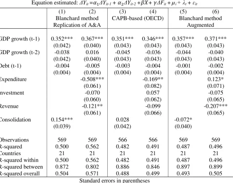
4. Endogeneity of fiscal indicators

This section analyzes and compares the cyclical behavior of the BFI (as estimated by

A&A, 2010) with ΔCAPB, as calculated by the OECD. Since section 2 has shown that

the BFI suffers from imperfect cyclical adjustment, hypothesis (1) is that the BFI entails

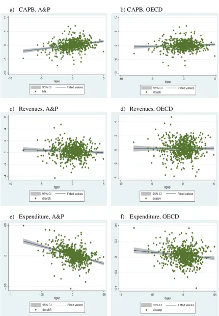
a (positive) cyclical pattern. Figure 1 compares a) changes in the CAPB (estimated

according to A&P), and b) according to the definitions of the OECD with changes in the output gap, since an imperfect c.a. problem would result in a (more) cyclical behavior of ΔCAPB.17

Figure 1 (c and d) depicts the cyclical behavior of cyclically adjusted government revenues (adjusted with the A&P method and the OECD method), and Figure 1 (e and f) shows the comparable behavior of expenditures. Figure 1 a) and b) show that the fiscal indicators measured according to A&P depict a more cyclical pattern, compared to the OECD fiscal indicator (hypothesis 1). While this pattern is not visible for revenues (1 c), it is particularly pronounced in the case of expenditures (hypothesis 2). We quantitatively explore the cyclical pattern of the fiscal indicators ΔFit in a panel

dataset (country i and year t) with regressions of the following form18

(17) ΔFit = µi + λt +𝛾ΔGapit + uit

Table 2 shows the estimated coefficients 𝛾. For comparison, Table 2 includes the

unadjusted primary balance as another reference. As expected, it is shown that the unadjusted primary balance entails a cyclical pattern (no cyclical adjustment). This pattern seems to be lower but persistent in the A&P measure (imperfect cyclical adjustment), while the CAPB of the OECD appears to be uncorrelated to changes in the economic cycle. The augmented BFI even depict a countercyclical behavior. Looking at government revenues, the unadjusted series are negatively correlated to the output gap,

17 _{The data used in this paper is from the same source as used in A&A (2010), obtained from the OECD}

Economic Outlook no. 84. The c.a. procedure of the OECD is described in Girouard and André (2005).

18 _{Guajardo et al. (2014) analyze fiscal cyclicality in a comparable framework to show that the CAPB (as}

15

pointing to a short-run elasticity of < 0. However, after applying any cyclical adjustment procedure, the cyclicality of revenues disappears.

However, as proposed by hypothesis 2, the indicators of government expenditures (as a ratio of GDP) are negatively associated with the economic cycle, which is strongly pronounced in the case of the unadjusted indicators. Adjusting the expenditure ratio

with the Blanchard-method (A&P), the counter-cyclical pattern remains at a slightly

lower level, while the relationship disappears after applying the OECD measure and even turns into opposite after applying the augmented version of the BFI. Thus, the A&P method does not sufficiently control for cyclical effects in government

expenditure, as suspected in equation (15).19

5. Large recessions and expansions

A&A (2010) identify episodes of large changes in fiscal policy. According to their definition, an episode of a large fiscal stimulus is an episode when the BFI (primary deficit, c.a. with the Blanchard method) increases by more than 1.5 pp. of GDP in the same year, while an episode of a large fiscal adjustment is an episode when the BFI (primary deficit, c.a. with the Blanchard method) decreases by more than 1.5 pp. of GDP. Following the hypotheses above, it is conceivable that the selection of these episodes is endogenous to economic growth. In particular, the identification as an episode of large fiscal stimulus will be influenced by negative changes in the output gap, while positive changes in the output gap will increase the likelihood of identifying this episode as a large fiscal consolidation.

Table 3 shows the 40 largest cases of economic recessions (negative changes in the output gap) in OECD history (in the dataset of A&A, 2010). While this selection focuses on episodes during the oil price crises of 1975 and 1981, some of these episodes are selected as large episodes of fiscal expansion, according to A&A (2010). To test whether this selection is based on the cyclical adjustment strategy of A&P, the BFI in these episodes is compared with the CAPB (c.a. with OECD method) and it is shown that the CAPB, as estimated with the OECD method, identifies several large recessions

19 _{The results are very much in line if we use GDP growth as an alternative cyclical indicator, rather than}

16

as episodes of discretionary fiscal stimulus, however several of the episodes identified by A&A (2010) are not large expansionary episodes if the CAPB of the OECD is used. For instance, Canada in 1982 and 1991, as well as Belgium and France in 1975 did not increase the CAPB by more than 1.5. percent, while A&A (2010) identify these years as episodes of large fiscal expansions (because the BFI increases by > 1.5 percent). This selection points to the two problems highlighted by Perotti (2013), the countercyclical response problem (a), as well as the incomplete cyclical adjustment problem (b).

First, the countercyclical response problem (a) appears if fiscal policy behaves countercyclical and increases deficits as a consequence of an economic recession. Table 3 depicts that this problem appears in both cases, whether we rely on the BFI or the CAPB. Governments tend to increase the CAPB in periods of economic slack as a countercyclical policy response, whether the cyclical adjustment strategy is the

Blanchard method or the OECD method. This countercyclical response problem is one

reason for the critique of the data-based approach. However, the CAPB (OECD method) selects substantially fewer recessions as episodes of fiscal stimuli, compared to the BFI. This, secondly, points to an incomplete cyclical adjustment problem (b) for the BFI (hypothesis 1). Since this article focuses on the question of how to correct for cyclical effects and whether an incomplete cyclical adjustment influences the results of the fiscal multiplier, we do not elaborate on the countercyclical response problem in more detail, but focus on the incomplete cyclical adjustment problem.

17

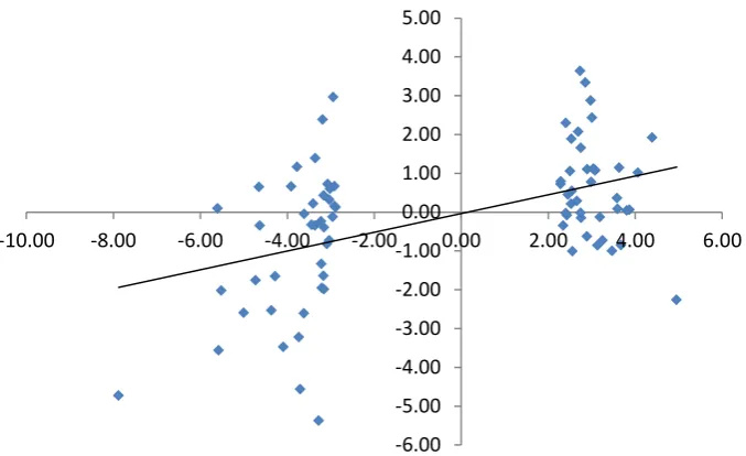
in which the BFI selects a large episode of economic expansion as period of fiscal consolidation significantly increases (more than doubled), so that the effect of the imperfect cyclical adjustment (in A&P) should not be underrated. Figure 2 shows the correlation between changes in the economic cycle (output gap) and the CAPB (based on the Blanchard method) in the 40 largest episodes of economic upswings and downturns. It shows a clear negative relationship, suggesting that the BFI-based CAPB tends to be clearly more expansionary in economic recessions, compared to the large episodes of economic upswings (when the BFI-based CAPB seems to be more contractionary). From this picture, it is reasonable to assume a positive correlation between fiscal adjustments and GDP (either through a countercyclical response problem or expansionary austerity).

Figure 3 depicts the same variables, but now the CAPB is calculated with standard assumptions of the OECD. The clear negative relationship decreases substantially. While the positive relationship is particularly pronounced in the case of economic downturns, it is less significant in the case of economic upswings, pointing to a small remaining countercyclical response problem in times of recessions (probably as a reaction to the oil price crises in 1975 and 1981), while there is little support for a large

countercyclical response problem in the case of upswing episodes.20

In summary, the CAPB based on the BFI appears to be highly correlated with changes in the economic cycle, while the CAPB based on conventional methods is not. This suggests that the BFI as proposed by A&P and applied by A&A (2010) suffers from an incomplete cyclical adjustment problem, as suggested by hypothesis (1). It is shown that the incomplete cyclical adjustment problem increases the likelihood of selecting an economic recession as a fiscal expansion and an economic upswing as an episode of fiscal consolidation.

20 _{The same is true if the BFI (as computed by A&A) is contrasted with the augmented version of the BFI,}

18

6. Replication and sensitivity of the results

This section reproduces the evidence shown in A&A (2010) based on the BFI and shows the sensitivity of the results if CAPB as a fiscal indicator is cyclically-adjusted

with different methods (A&P method vs. OECD method and augmented BFI). 21

As discussed in the previous section, A&A (2010) examine episodes of large changes in the fiscal stance, if the BFI/CAPB increases/decreases by more than 1.5 percentage points. The selected episodes by this definition, for the BFI, the CAPB (OECD), as well

as the augmented BFI, are shown in the appendix.22 Table 5 and 6 show the results of a

replication of A&A (2010) with the BFI, the CAPB (OECD), and the augmented BFI as a fiscal indicator. A&A (2010) analyze the effect of changes in the CAPB on GDP in episodes of large changes in the fiscal stance with regressions of the following form:

(18) _{it j it it}

j j

it y capb X u

y       

 _













2

1

Here, only cases of either large fiscal expansions or large fiscal consolidations are taken into account. Table 5 shows the results for the analysis of large episodes of fiscal expansions. While column (1) and (2) are perfect replications of the results in A&A, column (3) and (4) show the same results, with the only difference that the CAPB is used as provided by the OECD (from the OECD Economic outlook no. 84), rather than calculated with the A&P method. While the BFI (A&P) selects 72 episodes, the number of episodes selected by the CAPB (OECD) and the augmented BFI decreases substantially (65 and 64). While the positive (expansionary) effect of fiscal consolidations decreases after using the CAPB (OECD), the effect is not statistically significant in all three regressions (column 1, 3, 5). Column (2), (4) and (6) distinguish between the effect of current expenditure investment and revenue. The results based on the BFI and presented in A&A show a clear negative relationship between expenditure and growth in episodes of fiscal stimuli. This relationship has been widely interpreted as evidence for a negative multiplier in the case of expenditure cuts (A&A, 2010).

21 _{Since the data is the same data as used by A&A, the results for the Blanchard method are perfect}

replications of the results in A&A.

19

However, using the OECD measure of the CAPB, this result decreases substantially and loses statistical significance (column 4). In column 6 the coefficient for expenditures even turns into opposite, after applying the augmented specification of the BFI, suggesting that the BFI, if correctly specified, does not produce results in support of expansionary fiscal contractions in the case of expenditures.

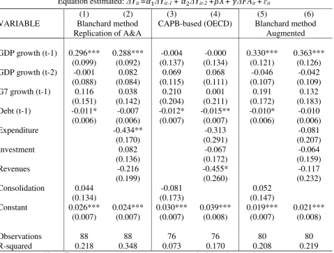
Table 6 illustrates the results for fiscal adjustments. As in the case of fiscal stimuli (Table 5), the number of observations decreases (from 88 to 76 / 80) after using the CAPB (or the augmented BFI). Similar to the evidence in Table 5, the effect of fiscal consolidation based on the BFI is positive in column 1, suggesting evidence for expansionary austerity. The results based on the CAPB (OECD), however, shows that fiscal consolidations appear to be negatively associated with GDP growth, suggesting a Keynesian effect. Nevertheless, again the effect is not statistically significant in all specifications. Column 2, 4 and 6 distinguish between the effects of expenditure- and revenue- based fiscal consolidations. It turns out that the effect of revenues increases slightly if the OECD method is applied, while the effect of expenditure cuts on GDP decreases and loses statistical significance if the cyclical adjustment is based on the OECD method. Again, the negative effect of expenditures disappears after applying the augmented version of the BFI (table 6). The negative multiplier for results based on the BFI seems to be more pronounced in the case of expenditure cuts, compared to increases in revenues (hypothesis 4), representing the countercyclical response problem. Further, the evidence presented in Tables 5 and 6 is based on a limited number of observations so that it might be interesting to additionally analyze and compare the evidence based on the full sample and not rely only on the selective evidence for cases of large changes in fiscal policy.

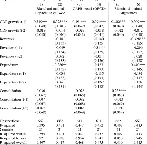
Table 7 replicates and compares another result of A&A (2010), that fiscal consolidations are positively associated with GDP, if the sample is not restricted to large episodes of discretionary change. We estimate regressions of the following form:

(19) it j k it k i t t

j j

it y capb u

y       

 _{ }





2









1

20

replication of the A&A results, while columns (3) and (4) show the results based on the CAPB (OECD), and (5) and (6) based on the augmented BFI. Comparing columns (1) and (3), the statistically significant positive effect of fiscal consolidation on GDP disappears after using the CAPB of the OECD (hypothesis 3). Using the augmented BFI, column (5) suggests that fiscal consolidations have negative rather than positive effects. Further, the negative multiplier for expenditures (column 2) decreases substantially if CAPB based measure rather than the BFI (column 4) is used and turns into opposite after using the augmented BFI (consistent with hypothesis 4).

7. Dynamic effects

This section includes dynamic effects of fiscal policy on GDP and investigates whether the results change after excluding large episodes of fiscal expansions and analyzing only episodes of large increases in the CAPB in a large panel of OECD countries. At the same time, we compare the results based on the three different methods to adjust for cyclical effects. To analyze the dynamic effects of fiscal consolidations on GDP and how this is influenced by the strategy of how to adjust for cyclical effects, we apply the method proposed by Leigh et al. (2010) and Alesina and Ardagna (2013):

(20) i t t

FA k it k

k j

it j

j

it y capb u

Y       

 _

 









2







0 2

1

Again, y_itrepresents real GDP growth in country i at time t and cab_itFA denotes the

estimated change in the cyclically adjusted primary balance (as a percentage of GDP) in

periods of large fiscal adjustments (capb_itk > 1.5 p.p. of GDP) and zero otherwise.23

As in chapter 5, we distinguish between three strategies to adjust for cyclical effects, the BFI method as proposed by Alesina and Perotti (1995), the conventional (OECD) method, as proposed by Girouard and André (2005), and the augmented BFI as

23 _{In an augmented specification I include changes in cyclically-adjusted current revenues and changes in}

21

proposed in section two of this paper.24 i and t represent cross-section and time

fixed effects, respectively.

Table 8 shows the results of this augmented specification. Since A&A (2010) did not compute dynamic responses of fiscal policy, this table is not a replication of A&A (2010), however, since the sample and data is almost similar, it is comparable to A&A (2013), where dynamic responses of changes in fiscal policy based on the BFI (A&P) are estimated within a similar framework.

Column (1) shows a positive association between fiscal adjustments and GDP growth, however, the result is not statistically significant. This coefficient changes its sign in column (3), after using the c.a. strategy of the OECD and after applying the augmented version of the BFI (column 5). Furthermore, column (2) shows a strong non-Keynesian effect of expenditure cuts on GDP (based on the BFI, according to A&A), but the result turns into opposite after using the OECD measure or the augmented BFI. This clearly supports hypothesis 3 and 4 which states that the BFI-based results are biased towards expansionary effects and that this bias is particularly pronounced for expenditure cuts. Column (4) and (6) additionally suggest that the (negative) effects of revenue-based consolidations are underestimated in the case of the BFI-based measure.

Figure 4 depicts the dynamic effects of changes in fiscal policy based on the results of equation (20), where there is a distinguishment between the estimated effect of large changes in the CAPB as calculated by the method proposed by A&P (1995) and large changes in the CAPB as provided by the OECD. Similar to A&A (2013), dynamic response functions are computed with the delta method, depicting the estimated response of GDP to a one-percentage point fiscal consolidation after a given period. According to the estimated regressions (table 8), the dynamic response varies with the measure of fiscal policy.

A comparison of the results show that the estimated contractionary effect of fiscal adjustments based on the CAPB (OECD approach) is more pronounced, compared to the results based on the A&A method. While the response of the BFI-based consolidation shows some evidence for potential expansionary effects of fiscal

24 _{The data and sample in this study again is the same as in A&A (2010), while the results for the}

22

adjustment, the results based on the CAPB (OECD approach) are relatively contractionary, in line with hypothesis (3).

Figure 5 shows the estimated effect of a one percent point increase in current revenues. In line with hypothesis 4, the estimated effects of both approaches are relatively similar and contractionary, what is not surprising, given that the elasticity of revenues is usually assumed to be approximately one, so that the revenue-GDP-ratio does not necessarily need to be adjusted for automatic cyclical effects.

Figure 6 shows the same results for expenditure cuts. The estimated effect of a one percent point reduction in primary expenditures is very different in both approaches, depending on the method applied to adjust the data for cyclical effects. The A&P approach finds expansionary effects of fiscal adjustments at the spending side. The (negative) impact multiplier is estimated to be -0.3 and turns out to be -0.4 after two

years.25 If the data provided by the OECD is used, the result is the opposite. The impact

multiplier is 0.1 (positive), suggesting that a reduction in government spending has a negative impact on GDP. This observation is in line with hypothesis (4), where a negative correlation is expected between GDP growth and the expenditure-GDP ratio, if

we fail to correct the expenditure-GDP ratio for cyclical effects.26

In this line, figure 7, 8, and 9 depict the response of GDP after a one percentage point fiscal consolidation, and compares the BFI-based (A&A) results with results based on the augmented BFI. Summarizing, the results support the view that the BFI as computed by A&A underestimates the contractionary effects of expenditure based consolidations. Since the conventional approach has been criticized for not controlling for one-off operations (Guajardo et al, 2014), an alternative CAPB of the OECD was used, which

excludes one-off operations, the so-called underlying balance.27 As a test for robustness,

all regressions are estimated using this indicator alternatively. After using the underlying balance, most of the results turn out to be even more pronounced and

25 _{These results are very much in line with the results in Alesina and Ardagna (2013), who found that a}

one percent point reduction in government spending increases GDP by 0.15 percent in the same year and by 0.46 percent after two years.

26 _{Alesina and Ardagna (2010) state that their results are not affected by the method applied to adjust for}

cyclical effects, and that the results remain robust, even without controlling for cyclical effects. Indeed, the estimated effects of fiscal consolidations based on the A&P approach are almost identical to those estimated with unadjusted data. To address this question, I compute the results based on unadjusted data, compared to the results based on the CAPB. The results based on this measure are available upon request.

27 _{Refer to Joumard et al. (2008) for a discussion on how one-off operations influence the budget balance}

23

statistically significant, compared to the CAPB-based ones.28 Nevertheless, since the

intention of this paper is the illustration of the incomplete cyclical adjustment problem in the literature following the method proposed by A&P (1995) at this point there is no extensive discussion on the advantages and disadvantages of using this alternative indicator.

8. Conclusion

A large share of empirical literature on fiscal policy using the conventional approach

pioneered by Alesina and Perotti (1995) examines changes in cyclically-adjusted budget balances (CAPB) and finds a positive relationship between CAPB (computed with the A&P-method) and GDP (non-Keynesian effects or expansionary austerity). This counter-intuitive relationship has been found to be particularly pronounced in the case of government spending (wage- and non-wage consumption expenditure). This stream of literature highlights that adjustments at the spending side are likely to be successful (in reducing government debt) or expansionary, while this is not the case for revenue-based consolidations (for example A&A, 1998, 2010 and 2013).

A number of authors have criticized these findings and pointed to potential conflicts with endogeneity. For instance, Jayadev and Konczal (2010) and De Cos and Moral-Benito (2013) found that the evidence on expansionary austerity in A&A (2010) is mainly based on successful adjustments in an economic upswing.

Guajardo et al. (2014) contrasted the data-based evidence in A&A (2010) with new evidence based on narrative measures of fiscal consolidations. They show that the data-based fiscal consolidations are correlated with economic growth forecast revisions. Nevertheless, the literature so far has not identified why the CAPB as proposed by A&P is endogenous to growth and how the assumptions made in A&P change the resulting estimated fiscal multiplier in data-based analyses of fiscal policy. Some studies highlight the presence of a countercyclical response problem (de Coz and Moral-Benito, 2013, and Guajardo et al., 2014), while others discuss the failure of the BFI to address the fiscal effects of changes in asset prices (Guajardo et al., 2014 and Yang et al., 2015). However, both hypotheses do not explain why the CAPB computed with other standard

24

methods is not (or less) endogenous to growth, a finding that is shown in this paper. The reverse causality argument can be seen as an answer to this puzzle.

The reverse causality argument proposed in this article focuses on the incomplete cyclical adjustment problem in the approach of A&P (1995) to adjust for cyclical effects

in budgetary data with the help of the “Blanchard method” to compute the Blanchard

fiscal indicator (BFI), which is relevant in a large number of subsequent studies based

on the same approach, as for instance A&A (1998, 2010 and 2013), as well as Ardagna (2002 and 2009). It is shown that the cyclical adjustment strategy pioneered by A&P

(1995) and applied in a number of subsequent articles is prone to an imperfect cyclical

adjustment problem (following the definition of Perotti, 2013). Only Holden and

Midthjell (2013) pointed to a potential reverse causality problem in A&A (2010) when analyzing whether fiscal policies might be successful in reducing government debt, but without discussing the assumptions made in A&P and how this affects the estimated fiscal multiplier.

The critique of the A&P method proposed in this paper is that A&P implicitly assume an elasticity of government expenditure (other than transfers) with respect to GDP of one (or close to one) when calculating the Blanchard Fiscal Indicator (BFI). Conversely, standard cyclical adjustment procedures assume an elasticity of zero for expenditures other than transfers (Girouard and André, 2005). The theoretical discussion in this paper states that the imperfect cyclical adjustment problem influences the estimated multiplier in conventional (data-based) analyses of fiscal policy so that the results are

endogenously biased towards expansionary austerity. This paper highlights that the results in A&A are affected by reverse causality, i.e. increasing GDP decreases expenditure-GDP-ratios, if the method applied fails to adjust for cyclical effects. It is shown theoretically and empirically that the cyclical adjustment strategy proposed by A&P does not appropriately control for cyclical effects.

25

It is shown that the CAPB based on the A&P method is positively correlated with changes in the economic cycle, while the CAPB based on conventional methods (and with the augmented version of the BFI) is not, pointing to the fact that the fiscal indicator used in A&A entails cyclical fluctuations and so the results of their approach are prone to reverse causality.

Investigating large changes in the output gap, it is shown that the strategy proposed by A&P increases the likelihood that a large episode of economic downturn is selected as an episode of a large fiscal stimulus by the method applied in A&A (2010), so that a large share of cases of fiscal stimuli as examined by A&A (2010) are affected by cyclical increases in deficits, rather than structural stimuli. In this line, the cyclical adjustment strategy proposed by A&P increases the likelihood that an episode of large economic upswing is selected as an episode of fiscal consolidation, since the cyclically adjustment procedure fails to disentangle the endogenous cyclical increase in the budget balance and the exogenous discretionary change in the fiscal stance. The imperfect cyclical adjustment problem particularly affects the expenditure-GDP-ratio, so that an increase in GDP is associated with decreases in the expenditure-GDP-ratio, while the (non-) adjustment of revenues in the approach of A&P does not affect the results in a systematic pattern.

26

contractive. While the latter finding is in line with the theoretical literature, the finding of expansionary effects in the case of expenditure cuts has been frequently highlighted in the academic debate as well as among policy-makers during the European fiscal crisis (see for example, BMF, 2012).

In this article it is shown that this finding reflects reverse causation, i.e. cyclical increases in the budget as a result of an economic upswing, rather than an economic upswing resulting from a discretionary cut in government expenditures.

This article might also contribute to the literature in a more general way. Some contributions have been critical regarding conventional analyses of fiscal policy in the recent past (Guajardo et al, 2014). Nevertheless, there is an urgent need to analyze budget data and to improve cyclical adjustment strategies to proxy discretionary changes in fiscal policy and to estimate cyclically-adjusted budget data, as for example in the context of the newly established fiscal rules in Europe.

27 References

Alesina, A. and S. Ardagna (1998), “Tales of Fiscal Adjustment”, Economic Policy 13,

489-585.

Alesina, A. and S. Ardagna (2010), “Large Changes in Fiscal Policy: Taxes vs.

Spending”, in: Brown, J. R. (ed.), Tax Policy and the Economy 24, Chicago: University

of Chicago Press, 35-68.

Alesina, A. and S. Ardagna (2013), “The Design of Fiscal Adjustments”, in: Brown, J.

R. (ed.), Tax Policy and the Economy 27, Chicago: University of Chicago Press, 19-67.

Alesina, A. and R. Perotti (1995), “Fiscal Expansions and Adjustments in OECD

Countries”, Economic Policy 10, 205-248.

Alesina, A. and R. Perotti (1997), “Fiscal Adjustments in OECD Countries:

Composition and Macroeconomic Effects”, NBER Working Paper 5730.

Ardagna, A. (2004), “Fiscal stabilizations: When do they work and why”, European Economic Review, 48, 1047-1074.

Ardagna, A. (2009), “Financial markets’ behavior around episodes of large changes in

the fiscal stance”, European Economic Review, 53, 37-55.

Blanchard, O. (1990), “Suggestions for a new set of fiscal indicators”, OECD Economics Department Working Paper No. 79.

BMF (2012), „Monatsbericht des BMF - November 2012“, German Federal Ministry of

Finance, 2012.

De Cos, P. H. and Moral-Benito, E. (2013), “Fiscal Consolidations and Economic

28

De Coz, P. H. and Moral-Benito, E. (2016), “On the predictability of narrative fiscal

adjustments”, Economics Letters, 143, 69-72.

Fedelino, A., Ivanova, A., Horton, M. (2009), “ Computing Cyclically Adjusted

Balances and Automatic Stabilizers”, International Monetary Fund, Technical Notes

and Manuals, 09/05.

Giavazzi, F. and M. Pagano (1990), “Can Severe Fiscal Contractions be Expansionay? Tales of Two Small European Countries”, NBER Macroeconomics Annual, 1990.

Giavazzi, F. (1995), “Comment on Fiscal Expansions and Adjustments in OECD

Countries”, Economic Policy, 1995, 240-241.

Girouard, N and C. André (2005), “Measuring cyclically-adjusted budget balances for

OECD countries”, OECD Economics Department Working Paper 434.

Guajardo, J., D. Leigh, and A. Pescatori (2014), “Expansionary Austerity? International

Evidence”, Journal of the European Economic Association, 12, 949-968.

Holden, S., Midthjell, N. L. (2013), „Successful Fiscal Adjustments – Does the Choice

of Fiscal Instruments Matter?”, CESifo Working paper Series 4456.

Jayadev, A. and M. Konczal (2010), “The Boom Not the Slump: The Right Time for

Austerity”, New York: Roosevelt Institute.

Jordà, Ò. and Taylor, A. (2015), “The Time for Austerity: Estimating the Average

Treatment Effect of Fiscal Policy”, Economic Journal, 2016, 126, 219-255.

Joumard, I., M. Minegishi, C. Andre, C. Nicq, and R. Price (2008), “Accounting for

one-off operations when assessing underlying fiscal positions”, OECD Economics

29

Kollintzas, T. (1995), “Comment on Fiscal Expansions and Adjustments in OECD Countries”, Economic Policy, 1995, 241-243.

Leigh, D., P. Devries, C. Freedman, J. Guajardo, Laxton, D. and A. Pescatori (2010),

“Will It Hurt? Macroeconomic Effects of Fiscal Policy Consolidation”, in: IMF World Economic Outlook October 2010, 93-124.

Morris, R., and L. Schuknecht (2007), “Structural balances and revenue windfalls: the role of asset prices revisited”, European Central Bank Working Paper, 737.

Stiglitz, J. (2016), “The Euro: How a common currency threatens the future of Europe”, New York: W. W. Norton & Company.

Perotti, R. (2013), “The “Austerity Myth”: Gain Without Pain?”, NBER Chapters, in:

Fiscal Policy after the Financial Crisis, NBER.

Yang, W., Fidrmuc, J., Ghosh, S. (2015), “Macroeconomic effects of fiscal adjustments:

30

Table 1: Consequences of imperfect cyclical adjustment under different

assumptions on revenue- and spending elasticities

If Relation to gap Effect on the estimated multiplier

R



>1 R/Y (positive) Underestimation of the (negative) revenue multiplier

R



<1 R/Y (negative) Overestimation of the (negative) revenue multiplier

G



>1 G/Y (positive) Overestimation of the (positive) expenditure multiplier

G

[image:31.595.80.486.146.274.2]



<1 G/Y (negative) Underestimation of the (positive) expenditure multiplier

Table 2: Fiscal policy and changes in the output gap

Equation estimated: ΔFit = µi + λt + 𝛾ΔGapit + ɛit

Measure of ΔF β s.e. R-squared Obs

ΔPB 0.350*** 0.061 0.298 669

ΔCAPB (BFI, A&A) 0.188*** 0.059 0.228 668

ΔCAPB (OECD) 0.019 0.052 0.160 653

ΔCAPB (Augmented BFI) -0.116** 0.055 0.168 668

Current revenues β s.e. R-squared Obs

ΔR -0.107* 0.060 0.179 669

ΔCAR (BFI, A&A) -0.063 0.046 0.122 668

ΔCAR (OECD) -0.006 0.055 0.168 653

ΔCAR (Augmented BFI) -0.031 0.047 0.120 668

Current expenditures β s.e. R-squared Obs

ΔE -0.409*** 0.062 0.540 669

ΔCAE (A&A) -0.222*** 0.047 0.331 668

ΔCAE (OECD) 0.007 0.042 0.255 668

ΔCAE (Augmented BFI) 0.092** 0.038 0.217 668

Notes: The table reports point estimates and heteroscedasticity-robust standard errors. All specifications contain full set of country and time fixed effects (not reported in the table).

[image:31.595.91.507.359.665.2]

[image:32.595.88.477.106.757.2]

31 Table 3: 40 largest cases of economic downturns

Country Year BFI DCAPB DGAP BFI>1.5 CAPB<-1.5

Finland 1991 4.73 -2.90 -7.88 1 1

Japan 1974 -0.09 0.69 -5.60

Italy 1975 3.56 -1.63 -5.58 1 1

Canada 1982 2.02 -1.20 -5.52 1

Portugal 1993 2.59 -2.34 -5.00 1 1

Finland 1992 1.75 -1.64 -4.73 1 1

Portugal 1984 -0.65 1.53 -4.65

United States 1982 0.34 -1.02 -4.63

Belgium 1975 2.53 0.34 -4.37 1

Canada 1991 1.65 -0.67 -4.28 1

Spain 1993 3.47 -0.48 -4.09 1

United Kingdom 1980 -0.66 1.79 -3.91

Greece 1987 -1.17 2.47 -3.78

Austria 1975 3.22 -2.16 -3.73 1 1

Sweden 1977 4.56 -3.16 -3.71 1 1

Australia 1991 2.61 -1.96 -3.62 1 1

United States 1974 0.05 -0.09 -3.61

Switzerland 1991 0.32 -0.09 -3.44

Ireland 1986 -0.22 1.50 -3.40

Austria 1978 0.35 0.44 -3.36

Ireland 1983 -1.39 3.42 -3.36

Japan 1998 5.38 -6.06 -3.28 1 1

United States 1980 0.24 -0.74 -3.23

United States 1975 1.34 -2.85 -3.22 1

France 1975 1.96 -0.52 -3.20 1

Portugal 1983 -2.39 3.91 -3.19

United Kingdom 1991 1.64 -0.62 -3.17 1

New Zealand 1991 -0.43 1.10 -3.16

Australia 1982 0.39 -0.10 -3.16

Denmark 1981 1.99 -1.36 -3.16 1

United Kingdom 1981 0.82 0.47 -3.09

Sweden 1993 -0.72 0.38 -3.07

Ireland 1991 0.73 0.06 -3.04

Austria 1981 -0.32 1.24 -3.03

United States 1991 -0.60 0.39 -3.02

Australia 1983 0.12 0.19 -2.96

Norway 1989 -2.97 -0.74 -2.94

United Kingdom 1974 -0.16 0.65 -2.91

Belgium 1993 -0.67 2.10 -2.91

[image:33.595.87.472.108.755.2]

32 Table 4: 40 largest cases of economic upswings

Country Year BFI DCAPB DGAP BFI<-1.5 DCAPB>1.5

United Kingdom 1973 2.26 -3.75 4.95

Portugal 1988 -1.92 1.12 4.39 1

Denmark 1976 -1.01 0.07 4.06

Ireland 1990 -0.06 -1.49 3.87

Greece 1978 -0.04 -1.09 3.81

United States 1984 0.85 0.02 3.67

Norway 1985 -1.15 0.37 3.63

Portugal 1989 -0.08 -0.88 3.59

Japan 1973 -0.36 -0.12 3.59

Finland 1979 1.00 -1.69 3.47

Portugal 1987 0.73 -1.09 3.25

Australia 1984 0.13 -0.22 3.19

Japan 1972 0.86 -1.77 3.13

Finland 1997 -1.07 1.14 3.08

Belgium 1973 -1.09 -0.32 3.07

Finland 1989 -1.12 0.21 3.04

Italy 1976 -2.43 2.15 3.01 1 1

Canada 1984 -0.77 -0.07 2.99

Spain 1987 -2.88 1.71 2.98 1 1

Ireland 1997 -1.10 0.15 2.90

Denmark 1994 0.62 -0.60 2.89

Finland 1988 -3.34 2.37 2.85 1 1

Japan 1988 0.15 -0.07 2.76

United Kingdom 1988 -1.66 0.63 2.75 1

Belgium 1976 0.02 -0.92 2.74

Denmark 1986 -3.64 3.55 2.73 1 1

New Zealand 1994 -2.07 1.40 2.69 1

Austria 1979 -0.29 -0.23 2.66

Greece 1988 1.01 -2.02 2.56

United States 1973 -0.55 0.40 2.55

New Zealand 1993 -1.89 1.05 2.53 1

Netherlands 1976 -0.21 0.83 2.53

Canada 1973 -1.06 0.47 2.50

Belgium 1988 -0.45 -0.81 2.45

United States 1978 0.08 0.17 2.43

Italy 1979 0.03 -0.61 2.41

Sweden 1984 -2.30 1.20 2.41 1

Ireland 1999 0.35 -1.27 2.34

Canada 1999 -0.79 0.33 2.29

[image:34.595.58.548.134.500.2]

33 Table 5: Fiscal Stimulus and Growth

Equation estimated: ΔYit =𝛼1ΔYit-1 + 𝛼2ΔYit-2 +𝛽𝑋+ 𝛾ΔFSit +ɛit

(1) (2) (3) (4) (5) (6)

Blanchard method

Replication of A&A CAPB-based (OECD) Blanchard method Augmented

GDP growth (t-1) 0.468*** 0.484*** 0.528*** 0.542*** 0.252 0.225

(0.147) (0.133) (0.165) (0.164) (0.185) (0.179)

GDP growth (t-2) -0.162 -0.081 -0.219 -0.245 -0.064 -0.160

(0.139) (0.134) (0.149) (0.151) (0.164) (0.164)

G7 growth (t-1) 0.364* 0.272 0.308 0.272 0.305 0.253

(0.202) (0.185) (0.232) (0.229) (0.232) (0.225)

Debt (t-1) -0.004 -0.007 -0.008 -0.014 -0.006 0.003

(0.008) (0.008) (0.011) (0.012) (0.009) (0.010)

Expenditure -0.751*** -0.367 0.214

(0.262) (0.433) (0.378)

Investment -0.255 0.144 -0.427*

(0.185) (0.225) (0.244)

Revenues -0.177 -0.189 -0.435

(0.285) (0.375) (0.380)

Consolidation 0.283 0.113 0.291

(0.187) (0.228) (0.247)

Constant 0.008 0.012 0.012 0.017 0.023** 0.014

(0.009) (0.009) (0.012) (0.013) (0.011) (0.012)

Observations 72 72 65 65 64 64

R-squared 0.282 0.428 0.285 0.332 0.117 0.208

Notes: The table reports point estimates and heteroscedasticity-robust standard errors. *** Significant at 1%, ** significant at 5%, * significant at 10%.

[image:35.595.62.542.137.499.2]

34 Table 6: Fiscal Adjustments and Growth

Equation estimated: ΔYit =𝛼1ΔYit-1 + 𝛼2ΔYit-2 +𝛽𝑋+ 𝛾ΔFAit +ɛit

(1) (2) (3) (4) (5) (6)

VARIABLE Blanchard method

Replication of A&A CAPB-based (OECD) Blanchard method Augmented

GDP growth (t-1) 0.296*** 0.288*** -0.004 -0.000 0.330*** 0.363***

(0.099) (0.092) (0.137) (0.134) (0.121) (0.126)

GDP growth (t-2) -0.001 0.082 0.069 0.068 -0.046 -0.042

(0.088) (0.084) (0.115) (0.111) (0.107) (0.109)

G7 growth (t-1) 0.116 0.038 0.210 0.001 0.191 0.132

(0.151) (0.142) (0.204) (0.211) (0.172) (0.183)

Debt (t-1) -0.011* -0.007 -0.012* -0.015** -0.010*