The behaviour of disaggregated output over the economic cycle

Munich Personal RePEc Archive

The behaviour of disaggregated output

over the economic cycle

Mashabela, Juliet and Raputsoane, Leroi

7 February 2018

Online at

https://mpra.ub.uni-muenchen.de/88847/

The behaviour of disaggregated output over the

economic cycle

Juliet Mashabela* and Leroi Raputsoane**

September 5, 2018

Abstract

This study examines the behaviour of disaggregated real output over the economic cycle in South Africa. Aggregate output as well as sectoral and industry level output are decom-posed into their transitory and permanent components. These components of output are then examined for their comovement with those of Aggregate output. The results of the transitory components generally show a strong positive comovement of aggregate output with output of all the economic sectors and majority of the industries. The results of the potential components generally show a weak positive comovement of Aggregate output with output of majority of the economic sectors and industries. The results particularly show a weak comovement of aggregate output and output of general government services as well as community, social and personal services sectors which highlights a laissez faire approach of government to economic management. The results also show no definite distinction of indus-tries, such as defensive, cyclical and sensitive indusindus-tries, in contrast to the finance literature.

JEL Classification: C11, D20, E32

Keywords: disaggregated output, Economic cycle, Commovement

*Juliet Mashabela, [email protected], Johannesburg **Leroi Raputsoane, [email protected], Pretoria

Introduction

Calibrating policy formulation as well as investment and consumption decisions to eco-nomic fluctuations necessitates an understanding of how different industries behave relative to the economic cycle. For instance, the European Central Bank (ECB). (2012) and Morgan Stanley Capital International (MSCI). (2014) asserts that the investment literature distin-guishes between types of industries, categorised into defensive, cyclical and sensitive indus-tries, by how they respond to economic fluctuations. Endogenous and exogenous shocks drive the phases of the economic cycle where the short term cycle is determined by demand side shocks while the long term cycle is determined by supply side shocks. The short term economic fluctuations, or idiosyncratic shocks, emanate from changes in monetary, financial and fiscal policies, consumer and business sentiment and labour market flexibility, or nominal rigidities. The long term economic fluctuations, or permanent shocks, emanate from changes in investment, innovation, technological advancement, privatisation, deregulation and mul-tilateral agreements. The discussion on macroeconomic shocks can be found in (Nelson and Plosser, 1982), Kydland and Prescott (1990), Nelson (2005) and Christiano et al. (2005) while Diebold and Rudebusch (1970), Blanchard et al. (1986) and Campbell and Mankiw (1987) discuss the interaction of macroeconomic policy and the economic cycle.

This study examines the behaviour of disaggregated real output over the economic cycle in South Africa. Aggregate output as well as sectoral and industry level output are decom-posed into their transitory and potential components. These components of sectoral and industry level output are then examined for their comovement with those of aggregate out-put, which approximates the total economy. The aim is to uncover the similarities as well as the differences in fluctuations, or procyclicality as opposed to countercyclicality, of sectoral and industry level output relative to output of the total economy over the short and long term horizons. This is important because economic policy formulation as well as investment and consumption decision making to influence the macroeconomic fluctuations of the econ-omy could have undesired results to the microeconomic fluctuations of the econecon-omy. This is particularly relevant for the economic sectors and industries whose fluctuations do not match the fluctuations of the total economy overtime. Thus, the paper is of particular interest to policy makers in that it promotes coherent sectoral and industry level policy formulation, together with investment and consumption decision making, in the economy.

The paper is organised as follows. Next is the discussion of the data. Then is the specification of the empirical model. This is followed by presentation of the empirical results and the discussion of the possible policy implications. Last is the conclusion.

Data

The transitory and potential components, or periodicities, are achieved by first decom-posing real output into the short term and the long term components using the Hodrick and Prescott (1997) filter. However, these short term and long term components still contain the volatile and the permanent components, respectively. Therefore, both the short term and the long term components are further decomposed to isolate the transitory and volatile component as well as the potential and permanent component, respectively. In this manner, the duration of the volatile component is calibrated as a period of less than 2 years, the transitory component is about 5 years, the potential component is about 10 years, while the permanent component is a period of more than 10 years. The periodicities are identified by calculating the number of years that each component data series complete a full cycle and are almost identical to those that are identified by the Business Cycle Dating Committee at the National Bureau of Economic Research (NBER). The economic cycle literature normally identifies 2 components while Baxter (1994) identifies 3 components that comprise the trend, cyclical and irregular components. The end point corrections are made to the components data series following Baxter and King (1999) as well as Kaiser and Maravall (2012).

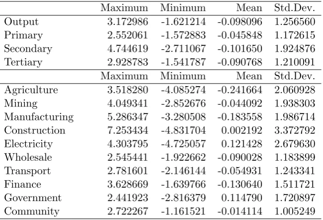
The descriptive statistics of the transitory components are presented in Table 1. The maximum value of aggregate output is about 3.2, mainly on account of real output of the secondary sector. The minimum value of aggregate output is about -1.6, also mainly on account of the secondary sector. As a result, the standard deviation of the secondary sector is the biggest compared to those of the primary and the secondary sectors implying higher volatility. The industries that realised the highest maximum values during the sample period are construction, manufacturing, mining and quarrying, as well as electricity, gas and water. In the same period, the highest minimum values were recorded by construction, electricity, gas and water, agriculture, forestry and fishing as well as manufacturing. The mean values of all the transitory components are about 0 given that all the components data series are deviations from their long term trend values. The transitory components of agriculture, forestry and fishing, construction, electricity, gas and water as well as mining and quarrying have the biggest standard deviations compared to those of the other industries.

Maximum Minimum Mean Std.Dev.

Output 3.172986 -1.621214 -0.098096 1.256560

Primary 2.552061 -1.572883 -0.045848 1.172615

Secondary 4.744619 -2.711067 -0.101650 1.924876

Tertiary 2.928783 -1.541787 -0.090768 1.210091

Maximum Minimum Mean Std.Dev.

Agriculture 3.518280 -4.085274 -0.241664 2.060928

Mining 4.049341 -2.852676 -0.044092 1.938303

Manufacturing 5.286347 -3.280508 -0.183558 1.986714 Construction 7.253434 -4.831704 0.002192 3.372792 Electricity 4.303795 -4.725057 0.121428 2.679630 Wholesale 2.545441 -1.922662 -0.090028 1.183899 Transport 2.781601 -2.146144 -0.054931 1.243341

Finance 3.628669 -1.639766 -0.130640 1.511721

Government 2.441923 -2.816379 0.114790 1.720897 Community 2.722267 -1.161521 -0.014114 1.005249

Notes: Own calculations with data from Statistics South Africa. Maximum measures the the biggest real GDP growth during the sample period, Mean shows the average GDP growth, Minimum is the smallest value of GDP growth and Std.Dev. is the standard deviation of GDP growth during the sample period.

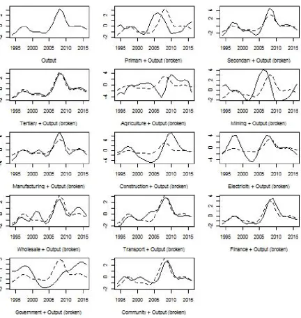
The graphs of the transitory components are depicted in Figure 1. The transitory com-ponent of aggregate output increased between 1994 and 1997 and then decreased from 1998 and reached a low in late 2003. It subsequently accelerated sharply reaching an all time high in late 2008 where it fell abruptly to 2012. The steady but slow growth of the transitory component of aggregate output between 2011 and 2014 was followed by the decrease to the end of the sample. The secondary and tertiary economic sectors tend to move particularly closely with aggregate output during the sample period while the opposite is true for the primary sector. Most economic industries move closely with aggregate output, in particular, wholesale trade, catering and accommodation, transport, storage and communication as well as finance, real estate and business services while the opposite is true for agriculture, forestry and fishing, mining and quarrying as well as general government services.

Notes: Own calculations with data from Statistics South Africa. The transitory components are measured as percentage deviation and are derived by isolating the volatile component from the short term component.

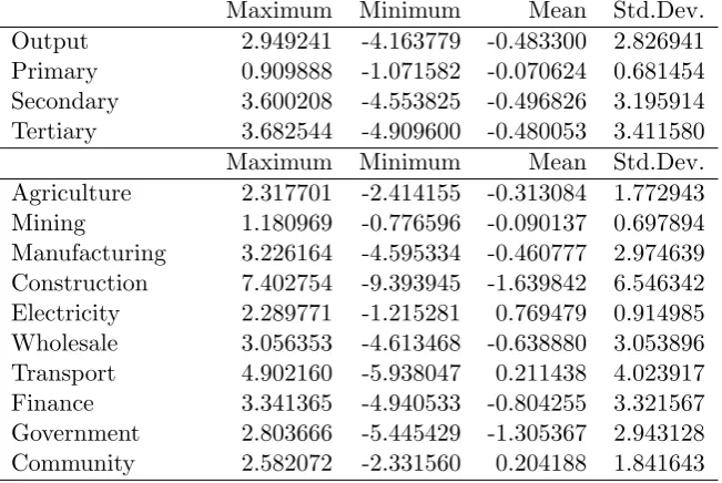
The descriptive statistics of the potential components are presented in Table 1. The maximum value of the potential component of aggregate output is about 2.9 during the sample period, mainly on account of real output of the secondary and tertiary sector. The minimum value of the potential component of aggregate output is about -4.2 during the sample period, also mainly on account of the secondary and tertiary sectors. As a result, the standard deviation of the secondary and tertiary sectors are the biggest compared to those of the primary sector. The industries that realised the biggest maximum values dur-ing the sample period are construction followed by transport, storage and communication. In the same period, construction, transport, storage and communication as well as general government services realised the biggest minimum values. The standard deviation of con-struction as well as transport, storage and communication were the biggest. The mean values of the potential components of most of the sectors and industries are negative so that the components generally declined during the sample period and hence their importance in the economy overtime. This is particularly the case with aggregate output as well as the output of the secondary and tertiary sectors, construction and general government services.

Maximum Minimum Mean Std.Dev.

Output 2.949241 -4.163779 -0.483300 2.826941

Primary 0.909888 -1.071582 -0.070624 0.681454

Secondary 3.600208 -4.553825 -0.496826 3.195914

Tertiary 3.682544 -4.909600 -0.480053 3.411580

Maximum Minimum Mean Std.Dev.

Agriculture 2.317701 -2.414155 -0.313084 1.772943

Mining 1.180969 -0.776596 -0.090137 0.697894

Manufacturing 3.226164 -4.595334 -0.460777 2.974639 Construction 7.402754 -9.393945 -1.639842 6.546342 Electricity 2.289771 -1.215281 0.769479 0.914985 Wholesale 3.056353 -4.613468 -0.638880 3.053896

Transport 4.902160 -5.938047 0.211438 4.023917

Finance 3.341365 -4.940533 -0.804255 3.321567

Government 2.803666 -5.445429 -1.305367 2.943128

Community 2.582072 -2.331560 0.204188 1.841643

Notes: Own calculations with data from Statistics South Africa. Maximum measures the the biggest real GDP growth during the sample period, Mean shows the average GDP growth, Minimum is the smallest value of GDP growth and Std.Dev. is the standard deviation of GDP growth during the sample period.

Table 2: Descriptive statistics of the potential component

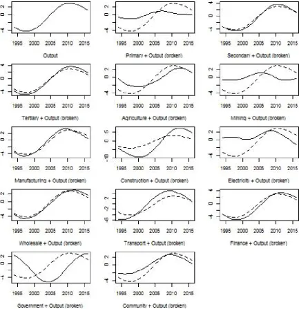
Notes: Own calculations with data from Statistics South Africa. The potential components are measured as percentage deviation and are derived by isolating the permanent component from the long term component.

Figure 2: Graphs of the potential components

Methodology

Hoeting et al. (1999), Bayesian Model Averaging (BMA) efficiently minimises the estimated parameters towards the stylised representation of the data leading to sound inference.

The Bayesian Model Averaging (BMA) empirical model is specified following Feldkircher and Zeugner (2015) where the details can be found. Given a vector of the dependent vari-able yt, which contains the transitory and potential components of output, and a matrix of

explanatory variablesXt, which contains the transitory and potential components of

disag-gregated real output, Bayesian Model Averaging (BMA) model is specified as follows

yt=αγt+Xγtβγt+ǫt , ǫt∼N 0, σ2

(1)

where αγt is a constant, βγt are coefficients, ǫt is the error term with mean 0 and variance

σ2_{. In the event of high dimensional data, the variable selection approach estimates all the} possible combinations ofXγt and constructs a weighted average over them to circumvent the

problem of identifying the explanatory variables to include in the model. ThusXγtcontains

K variables where 2K _{variable combinations are estimated and hence 2}K _models.

The model weights for Bayesian Model Averaging (BMA) are derived from posterior model probabilities using Bayes theorem as follows

p(Mγ |y, X) =

p(y|Mγ, X)p(Mγ)

p(y|X) =

(y|Mγ, X)p(Mγ)

P₂K

γ=1p(y|Ms, X)p(Ms)

(2)

wherep(Mγ|y, X) is the posterior model probability,Mγis the true model,p(y|Mγ, X) is

the marginal likelihood of the model, p(Mγ) is prior model probability and p(y|X) is the

constant integrated likelihood over all models. The Posterior Model Probability (PMP) is

p(y|X)p(βγ|y, X) =

2K

X

γ=1

p(βγ |Mγ, y, X)p(Mγ|y, X) (3)

whereβγ are the parameters of the model. The unconditional coefficients of the model are

E(βγ |y, X) =

2K

X

γ=1

p(βγ|Mγ, y, X)p(Mγ |y, X) (4)

where the Prior Model Probability (PMP) has to be proposed based on prior knowledge or believe. According to Varian (2014), Bayesian Model Averaging (BMA) analyses models with high dimensional data revealing the interdependence among the variables hence the method leads to a new way of understanding the underlying relationships among the variables.

Results

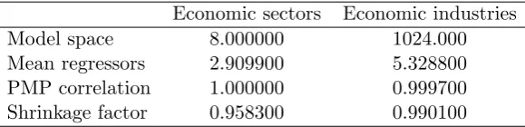
The model statistics of the comovement between the transitory components are presented in Table 3. The model space is 8.000 and 1024.000 given the 3 economic sectors and 10 economic industries, respectively. The mean number of regressors, which shows the average number of regressors with relatively high probability of inclusion in the estimated models, is 2.900 for the economic sectors model and 5.329 for the economic industries model. Thus economomic sectors and the economic industries models predict about 2 and 5 variables on average, repsectively, with high probability of inclusion in the estimated models. PMP Correlation shows that the degree of convergence between the prior and the posterior model probabilities is reasonably high for all the estimated models at 1.000 for the economic sectors model and 1.000 for the economic industries model. The Shrinkage factor, which is a goodness of fit indicator, is 0.958 for the economic sectors model and is 0.990 for the economic industries model. These show an almost perfect goodness of fit for both the estimated models.

Economic sectors Economic industries

Model space 8.000000 1024.000

Mean regressors 2.909900 5.328800

PMP correlation 1.000000 0.999700

Shrinkage factor 0.958300 0.990100

Notes: Own calculations with data from Statistics South Africa. Model space measures the variable com-binations in the estimated models. Mean Regressors are covariates with high probability of inclusion in the estimated models. PMP Correlation is the degree of convergence between the prior model probability and posterior model probability and Shrinkage Factor is the goodness of fit indicator of the estimated models.

Table 3: Model statistics of the transitory components

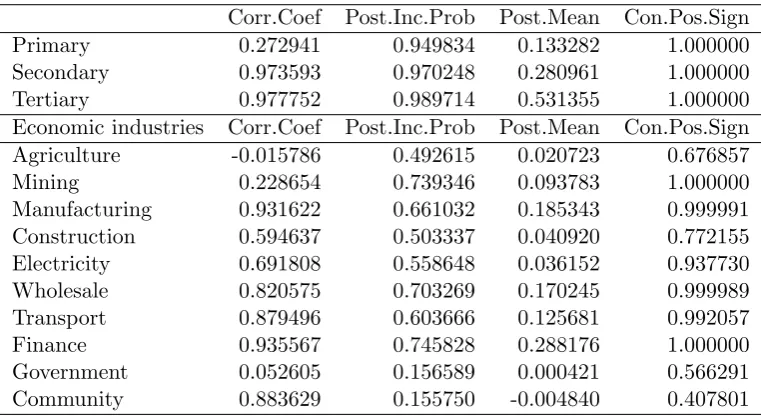
The results of the comovement between the transitory components are presented in Table 4. The top panel presents the results of the economic sectors while the bottom panel presents the results of the economic industries. The results of the economic sectors show a strong positive correlation between the secondary and tertiary sectors and aggregate output, while it shows a weak positive correlation of the primary sector and the aggregate output. The posterior inclusion probabilities show that the primary, secondary and tertiary sectors are included in over 90 percent of the models that explain aggregate output. The posterior mean shows that a 1 percent increase in transitory component of primary, secondary and tertiary sectors is associated with 0.133, 0.281 and 0.531 percent increase in the aggregate output, respectively. The conditional position signs of the main sectors are all 1.000, which show a 100 percent certainty of a positive relationship between output of the economic sectors and aggregate output. The results of the main economic industries show a strong correlation be-tween the manufacturing,transport, storage and communication as well as finance, real estate and business services with the aggregate output. Mining and quarrying as well as general government services show a weak correlation with the aggregate output while agriculture, forestry and fishing show virtually no correlation with the economic cycle.

The conditional position signs show a strong probability of a positive relationship between all the economic sectors and most economic industries, that include Mining and quarrying as well as finance, real estate and business services, and aggregate output. The opposite is true for agriculture, forestry and fishing as well as general government services which show a weak probability of a positive relationship with real output while community and personal services show a weak probability of a negative relationship with aggregate output.

Corr.Coef Post.Inc.Prob Post.Mean Con.Pos.Sign

Primary 0.272941 0.949834 0.133282 1.000000

Secondary 0.973593 0.970248 0.280961 1.000000

Tertiary 0.977752 0.989714 0.531355 1.000000

Economic industries Corr.Coef Post.Inc.Prob Post.Mean Con.Pos.Sign

Agriculture -0.015786 0.492615 0.020723 0.676857

Mining 0.228654 0.739346 0.093783 1.000000

Manufacturing 0.931622 0.661032 0.185343 0.999991

Construction 0.594637 0.503337 0.040920 0.772155

Electricity 0.691808 0.558648 0.036152 0.937730

Wholesale 0.820575 0.703269 0.170245 0.999989

Transport 0.879496 0.603666 0.125681 0.992057

Finance 0.935567 0.745828 0.288176 1.000000

Government 0.052605 0.156589 0.000421 0.566291

Community 0.883629 0.155750 -0.004840 0.407801

Notes: Own calculations with data from Statistics South Africa. Corr.Coef is the correlation coefficient and the associated p value, Post.Inc.Prob is the posterior inclusion probability, Post.Mean is the posterior mean and the associated posterior standard deviation and Con.Pos.Sign is the probability ofpositive coefficient.

Table 4: Model results of the transitory components

The model statistics of the comovement between the potential components are presented in Table 5. The model space is 8.000 and 1024.000 given the 3 economic sectors and 10 economic industries, respectively, as above. The mean number of regressors, which shows the average number of regressors with relatively high probability of inclusion in the estimated models, is 1.436 for the economic sectors model and 2.347 for the economic industries model. Thus economomic sectors and the economic industries models predict about 1 and 2 variables on average, repsectively, with a high probability of inclusion in the estimated models. PMP Correlation shows that the degree of convergence between the prior and the posterior model probabilities is reasonably high for all the estimated models at 1.000 for the economic sectors model and 1.000 for the economic industries model. The Shrinkage factor, which is a goodness of fit indicator, is 0.958 for the economic sectors model and 0.990 for the economic industries model. These th show an almost perfect goodness of fit for the estimated models.

Economic sectors Economic industries

Modelspace 8.000000 1024.000

Mean Regressors 1.436100 2.347000

PMP Correlation 1.000000 0.999800

Shrinkage Factor 0.958300 0.990100

Notes: Own calculations with data from Statistics South Africa. Model space measures the variable com-binations in the estimated models. Mean Regressors are covariates with high probability of inclusion in the estimated models. PMP Correlation is the degree of convergence between the prior model probability and posterior model probability and Shrinkage Factor is the goodness of fit indicator of the estimated models.

Table 5: Model statistics of the potential components

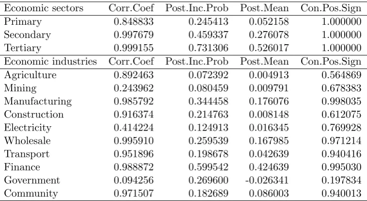
position signs of all the main sectors are all 1.000, which show a 100 percent certainty of a positive relationship of the primary, secondary and tertiary sectors with the aggregate output. The results of the economic industries show a strong positive correlation between most of the industries with the aggregate output, in particular, manufacturing, wholesale, retail trade and accommodation, transport, storage and communication as well as finance, real estate and business services industries. Mining and quarrying show a weak correlation with the aggregate output and no correlation for general government services.

Economic sectors Corr.Coef Post.Inc.Prob Post.Mean Con.Pos.Sign

Primary 0.848833 0.245413 0.052158 1.000000

Secondary 0.997679 0.459337 0.276078 1.000000

Tertiary 0.999155 0.731306 0.526017 1.000000

Economic industries Corr.Coef Post.Inc.Prob Post.Mean Con.Pos.Sign

Agriculture 0.892463 0.072392 0.004913 0.564869

Mining 0.243962 0.080459 0.009791 0.678383

Manufacturing 0.985792 0.344458 0.176076 0.998035

Construction 0.916374 0.214763 0.008148 0.612075

Electricity 0.414224 0.124913 0.016345 0.769928

Wholesale 0.995910 0.259539 0.167985 0.971214

Transport 0.951896 0.198678 0.042639 0.940416

Finance 0.988872 0.599542 0.424639 0.995030

Government 0.094256 0.269600 -0.026341 0.197834

Community 0.971507 0.182689 0.086003 0.940013

Notes: Own calculations with data from Statistics South Africa. Corr.Coef is the correlation coefficient and the associated p value, Post.Inc.Prob is the posterior inclusion probability, Post.Mean is the posterior mean and the associated posterior standard deviation and Con.Pos.Sign is the probability ofpositive coefficient.

Table 6: Model results of the potential components

no increase in aggregate output. The conditional position signs show a strong probability of a positive relationship between most economic industries and aggregate output, while the opposite is true for agriculture, forestry and fishing. General government services show a relatively strong probability of a negative relationship with aggregate output.

As discussed above, calibrating policy, investment and consumption decisions to economic fluctuations necessitates an understanding of how different industries behave relative to the economic cycle. This is because industries respond differently to economic fluctuations hence the comovement of different industries in the economy may be because they are driven, to a large extent, by common shocks. The results have provided evidence of a generally strong positive relationship between the transitory and potential components of the tertiary sector, in particularly, the finance, real estate and business services industry, while the opposite is true for the transitory and potential components of the primary sector, in particular, the agriculture, forestry and fishing industry. Contrary to the investment literature, there does not seem to be a clear distinction between the different economic industries by categories, such as the defensive, cyclical and sensitive industries. Consequently, the paper has enhanced the understanding of how the different economic sectors and economic industries behave relative to the economic cycle in quest to promote coherent sectoral and industry level policy formulation as well as investment and consumption decision making in the economy.

Conclusion

This study examined the behaviour of disaggregated sectoral and industry output over the economic cycle in South Africa. aggregate output as well as sectoral and industry level out-put were decomposed into their transitory and permanent components. The transitory and potential components of the economic sectors and economic industries were then examined for their comovement with those of the total economy. The results of the transitory com-ponents show a strong positive comovement between all the economic sectors and aggregate output. They further show somewhat strong positive comovement of the Mining and quar-rying, wholesale, retail trade and accommodation as well as finance, real estate and business services industries and aggregate output, while the opposite is true for general government services and community, social and personal services industries. The results of the potential components show a somewhat strong positive comovement between the tertiary sector and aggregate output while that of the primary and secondary sectors is weak. They further show a moderate positive comovement with the finance, real estate and business services industry while the comovement with the rest of the industries is weak. Contrary to the investment literature, there does not seem to be a clear distinction between the economic industries by categories, such as defensive, cyclical and sensitive industries. A weak comovement of general government services and community, social and personal services industries with aggregate output show a laissez faire approach to economic management by government.

References

Bartels, L. M. (1997). Specification Uncertainty and Model Averaging. American Journal of Political Science, 41(2):641–674.

Baxter, M. (1994). Real Exchange Rates and Real Interest Differentials: Have We Missed the Business Cycle Relationship? Journal of Monetary Economics, 33(1):5–37.

Blanchard, O. J., Hall, R. E., and Hubbard, R. G. (1986). Market Structure and Macroeco-nomic Fluctuations. Brookings Papers on Economic Activity, 1986(2):285–338.

Burns, A. F. and Mitchell, W. C. (1946). Measuring Business Cycles. NBER Books. National Bureau of Economic Research Inc.

Campbell, J. Y. and Mankiw, N. G. (1987). Permanent and Transitory Components in Macroeconomic Fluctuations. American Economic Review, 77(2):111–117.

Christiano, L. J., Eichenbaum, M., and Evans, C. L. (2005). Nominal Rigidities and the Dynamic Effects of a Shock to Monetary Policy. Journal of Political Economy, 113(1):1– 45.

Diebold, F. X. and Rudebusch, G. D. (1970). Measuring Business Cycles: A Modern Per-spective. Review of Economics and Statistics, 78(1):67–F77.

European Central Bank (ECB). (2012). Stock Prices and Economic Growth. Monthly Bul-letin, October.

Feldkircher, M. and Zeugner, S. (2015). Bayesian Model Averaging Employing Fixed and Flexible Priors. Journal of Statistical Software, 68(4):1–37.

Hodrick, R. and Prescott, E. C. (1997). Postwar U.S. Business Cycles: An Empirical Inves-tigation. Journal of Money, Credit and Banking, 29(1):1–16.

Hoeting, J. A., Madigan, D., Raftery, A. E., and Volinsky, C. T. (1999). Bayesian Model Averaging: A Tutorial. Statistical Science, 44(4):382–401.

Kaiser, R. and Maravall, A. (2012). Measuring Business Cycles in Economic Time Series, volume 154. Springer Science and Business Media, 3 edition.

Kydland, F. E. and Prescott, E. C. (1990). Business Cycles: Real Facts and a Monetary Myth. Quarterly Review, 4:3–18. Federal Reserve Bank of Minneapolis.

Leamer, E. E. (1978).Specification Searches: Ad Hoc Inference with Non Experimental Data. John Wiley and Sons Inc.

Morgan Stanley Capital International (MSCI). (2014). Cyclical and Defensive Sectors. In-dexes Methodology, June. Morgan Stanley Capital International.

Nelson, C. R. and Plosser, C. R. (1982). Trends and Random Walks in Macroeconomic Time Series: Some Evidence and Implications. Journal of Monetary Economics, 10(2):139–162.

Nelson, E. (2005). Monetary Policy Neglect and the Great Inflation in Canada, Australia and New Zealand. International Journal of Central Banking, 1(1):133–179.

Romer, C. D. (1993). Business Cycles. In Henderson, D. R., editor,The Fortune: Encyclo-pedia of Economics, volume 330.03 F745f. Warner Books.

Stock, J. H. and Watson, M. W. (1999). Business Cycle Fluctuations in US Macroeconomic Time Series. Handbook of Macroeconomics, 1(Part A):3–64.

Varian, H. R. (2014). Big Data: New Tricks for Econometrics. Journal of Economic Per-spectives, 28(2):3–28.