Munich Personal RePEc Archive
Development of a two-sector model with
an extended energy sector and
application to Portugal (1960-2014)
Santos, João and Domingos, Tiago and Sousa, Tânia and
Serrenho, André
MARETEC - Marine, Environment and Technology Center,
7 September 2018
Online at
https://mpra.ub.uni-muenchen.de/89175/
Development of a two-sector model
with an extended energy sector and
application to Portugal (1960-2014)
Authors:
João Santosa (corresponding author; e-mail: [email protected]) Tiago Domingosa (e-mail: [email protected])
Tânia Sousaa (e-mail: [email protected]) André Serrenhob (e-mail: [email protected])
Affiliations:
aMARETEC – Marine, Environment and Technology Center, Environment and Energy Scientific Area, Department of Mechanical Engineering, Instituto Superior Técnico (IST), University of Lisbon, Avenida Rovisco Pais 1, 1049-001 Lisbon, Portugal.
Abstract
In basic economic growth models, energy is neglected as a production factor, and output is generated from capital and labor in a single-sector process, with most of growth attributed to an exogenous residual. However, alternative approaches argue for a multi-sector system in which the major contribution to growth comes from increased efficiency in the conversion of energy to more productive forms.
In this work we develop a two-sector model for the economy, featuring an extended energy sector, including all primary-to-final (energy industries) and final-to-useful (end-use devices) exergy conversion processes. Exergy is a thermodynamics concept, accounting for the potential of energy to perform work. Empirical application of the model for a single country (Portugal) requires decomposition and reclassification of national accounts and energy balances, to match empirical data with the model’s variables.
Obtained estimates for the price of useful exergy (an intermediate product) facilitate the construction of gross output measures for more accurate growth accounting. Evidence suggests that declining useful exergy prices act as an engine of growth, as previously suggested in the literature. Additionally, useful exergy and capital inputs to non-energy related production act as complements while capital productivity in useful exergy generation declines slightly in the past decade.
Keywords
Two-sector model; extended energy sector; useful exergy; national accounts; energy balances;
Highlights
- A two-sector model, with an innovative extended energy sector, is developed; - The extended energy sector covers primary-to-final-to-useful exergy conversions; - National accounts and energy balances are reclassified to match model’s variables; - Declining useful exergy prices support positive feedback cycle as driver of growth; - Evidence of useful exergy and capital as complementary inputs to non-energy sector;
JEL Codes
1.
Introduction
Energy is essential to economic activity, and advances in energy consuming technologies, coupled with increasing energy consumption, have characterized industrialization and economic development over the past century. Despite this apparently close relationship, the standard theory of economic growth does not reflect energy availability or prices and fails to satisfactorily explain historical growth and productivity declines following energy crises.
The first and foremost goal of this work is to establish the basis for the development of a macroeconomic growth model that considers the real contribution of energy inputs to production processes and growth. The proposed model is built around several arguments regarding the role of energy in the economy – voiced mostly in the ecological economics literature – as well as recent empirical results supporting those same arguments. With the development of the model, we seek to provide new insights to persistent questions in the field of macroeconomics, such as the explanation for historical economic growth and recent productivity slowdowns verified in industrialized countries, as well as in regard to the relations between energy use, energy efficiency, energy prices, the traditional factors of production (physical capital and human labor), economic output, and growth. Overall, the proposed model aims to provide an improved characterization of economic and growth processes without disregarding an arguably essential input to the economic system: energy.
Section 1.1 begins by exposing the historical economic growth accounting method attached to most basic mainstream growth models (1.1.1) and subsequently highlighting some of the criticism imposed on these models concerning their inability to fully account for growth without an exogenous residual term (total factor productivity, or TFP) and the neglect of energy inputs, as opposed to alternative approaches that posit a central role for energy in economic understanding (1.1.2). Section 1.2 expands on the link between energy use – especially energy efficiency – and economic growth, invoking the thermodynamically defined useful exergy concept as the appropriate measure to account for productive energy uses. This subsection also reviews some of the more recently published evidence for useful exergy consumption as an explanatory factor of economic growth and states the case for the macroeconomic model developed in this work, based on the quantitative and qualitative evidence cited in regard to the relationship between productive energy and growth.
1.1.
The main(stream) driver of economic growth: total factor productivity
Basic mainstream economic growth theory generally attributes long-run growth to three major factors: 1) accumulation of capital; 2) increases in labor inputs, i.e. number of workers and/or hours worked; 3) technical change. The contribution from these factors to growth can be measured through growth accounting exercises, breaking down what percentage of growth can be attributed to changes in each of the factors.1.1.1. Growth accounting and the Solow residual
The Solow-Swan model – developed independently in two pathbreaking papers of the same year (Solow, 1956; Swan, 1956) – has shaped the field of macroeconomics and the way economic growth is approached. At the center of the model is a neoclassical aggregate production function (APF), linking a given level of economic output (𝑌) with a combination of inputs to production:
Physical capital (𝐾) and human labor (𝐿) are generally considered the primary factors of production in modern economiesi. The term 𝐴 is a “catch all” factor representing technology, institutional factors, and other forces that account for how productively capital and labor are used. Standard assumptions on the form of the APF include homogeneity of degree one and constant returns to scale, which in turn facilitates the assumption of perfect competition i.e. factors of production are paid their marginal productsii. The growth accounting equation is obtained from differentiating the APF in Equation (1) with respect to time, denoting growth rates by 𝑔 = 𝑑𝑖/𝑖:
𝑔 = (𝐹 𝐴/𝑌) ∙ 𝑔 + (𝐹 𝐾/𝑌) ∙ 𝑔 + (𝐹 𝐿/𝑌) ∙ 𝑔 , (2)
where 𝐹 denotes the partial derivative with respect to factor 𝑖. From perfect competition,
𝐹 = 𝑟 (rents – the marginal product of capital) and 𝐹 = 𝑤 (wages – the marginal product of labor). Simplifying Equation (2), the share of total income allocated to capital can be denoted by 𝛼 = 𝑟𝐾/𝑌, and the share allocated to labor by 1 − 𝛼 = 𝑤𝐿/𝑌.
𝑔 = (𝐹 𝐴/𝑌) ∙ 𝑔 + 𝛼 ∙ 𝑔 + (1 − 𝛼) ∙ 𝑔 (3)
The growth accounting methodology as expressed in Equation (3) – introduced by Robert Solow (Solow, 1957) – decomposes the growth rate of an economy’s total output into that which is due to increases in the contributing amount of the factors used, and that which cannot be accounted for by observable changes in factor utilization. In principle, with the exception of the first term, all terms in Equation (3) are directly observable and can be measured using standard national income accounting methods. However, the “technological” term (𝐹 𝐴/𝑌) ∙ 𝑔 is not directly observable as it captures improvements in productivity unrelated to changes in the use of factors of productioniii. This term is commonly referred to in the literature as the “Solow residual”, or total factor productivity (TFP).
Empirically, the construction of long time series for labor, capital, and gross domestic product (GDP) data allowed economists to apply the growth accounting technique to virtually every economy in the world (Crafts 2004; van Ark & Crafts 1996; Crafts 2009), and to develop quantitative factor productivity indices (Fabricant, 1954; Abramovitz, 1956; Schmookler, 1962). A common finding from these efforts is that increasing factor inputs – population, savings, and capital accumulation per se – cannot fully account for observed levels of economic growth in most industrialized economies. For the US, using time series data from 1909 through 1949,
Solow (1957) estimated that TFP accounted for more than 85% of per-capita growth. The TFP term has also been identified as the major driver of growth within other industrialized countries (Easterly & Levine, 2001).
1.1.2. Limitations of growth accounting and TFP methods
TFP as a “measure of our ignorance”
together” and cannot be sorted out within the growth accounting frameworkv. The Solow-Swan growth model itself does not seek to explain or derive the empirical residual, rendering it an exogenous black box, outside the model and the influence of economic incentives.
In an attempt to overcome the shortcomings brought by the treatment of innovation (in the form of changes in TFP) as exogenous to the growth modelvi, endogenous growth theory – as formulated by Romer (1986) and Lucas (1988) – expands the concept of capital to include knowledge and human capital, thus recognizing that some part of innovation is, in fact, a form of capital accumulation, and therefore endogenous to the model. In these models, growth is mostly due to indefinite investment in human capital which has a spillover effect on the economy and reduces the diminishing returns to capital accumulation (Barro & Sala-i-Martin, 2004). Such models imply that the long-run growth rate of an economy is promoted by policies that increase incentives to innovation.
However, the endogenous approach is not without its critics. The main failings pointed to these theories of growth concern the inability to explain the income divergence between the developing and developed economies (Sachs & Warner, 1997), and the phenomenon of conditional convergence verified in the empirical literature (Parente, 2001). Furthermore, endogenous growth theories also fail to offer a satisfactory explanation for the so-called “productivity conundrum” verified in developed countries. This phenomenon is characterized by a long-term and sustained slowdown of productivity growth, as has been the case for the world’s industrialized economies since the Great Recession of late 2000s. This slow rate of growth is even more puzzling because it has not been reversed by the “information revolution” brought by fast advances in digital and other information and communication technologies (ICT)vii. Secular stagnation theory attributes this slowdown not to cyclical or short-term depressions, but to a change of fundamental dynamics allowing for the possibility that “depression may become the normal condition of the economy” (Harris, 1943). While economists remain puzzled to the causes of this slowdown, possible explanations include Robert Gordon’s thesis that the periods of fast economic growth in the last century were fueled by large-scale innovations which are unrepeatable (i.e. the internal combustion engine, electrification, public sanitation) (Gordon, 2017). Other explanations focus on limits to productivity growth imposed by decreased competition, excessive regulation, or a slowing of gains in human capital, or mis-measurements in productivity gains (Baily & Montalbano, 2016). In the endogenous growth view, a productivity slowdown could be due either to a slowdown in the growth rate of generalized capital inputs, or to a decline in the spillover effect. However, neither case is supported by empirical evidence.
Energy inputs and its importance in economic production and growth
justify declines in output as an effect of reduced labor hours – itself a consequence, not a cause, of the declines.
[image:8.612.155.454.299.526.2]In this sense, Ayres (2001) emphasizes the importance of a positive feedback mechanism as a driver of growth, powered by cheap energy sources. Growth is endogenized with this cycle, which operates as follows: cheaper energy resource inputs, due to discoveries, economies of scale and experience (or learning-by-doing) enable tangible goods and intangible services to be produced and delivered at ever lower cost, i.e. resource (energy) flows are productive; lower costs in competitive markets translate into lower prices for products and services; through price elasticity effects, lower prices encourage demand; since demand for final goods and services corresponds to the sum of factor payments – most of which go back to labor as wages and salaries – it follows that wages of labor tend to increase as output rises; this, in turn, stimulates further substitution of energy resources and mechanical power produced from these resources, for human and animal labor; the continuing substitution drives further increases in scale, experience, learning, and lower energy resource costs still, thus closing the loop. A representation of this positive feedback cycle is given in Figure 1.
Figure 1 – Generalized positive feedback cycle. [Source: Warr & Ayres, 2006]
The reasoning behind this neglect of energy inputs in the standard growth theory framework stems from the argument that fuels and materials are not primary factors of production (such as capital, labor, and sometimes land), but intermediate inputs, which are produced by some combination of capital investment and labor (plus “technology”). This has led to a focus on the primary factors of production, and a much more indirect treatment of the role of energy. The prices paid for all the different inputs are seen as eventually being payments to the owners of the primary inputs for the services provided directly or embodied in intermediate inputs. Payments to capital (rents, interests) and labor (wages, salaries) are adequately represented in standard national accounts, but payments to energy resources are generally underreported in these statistics, and even then, are roughly equated with revenues from the energy industries, corresponding to less than 10% of income (US EIA, 2011; Platchkov & Pollitt, 2011). Denison (1979), among others, relied on this small cost share for energy to argue that energy prices could not have a significant impact on economic output and growth, and hence to justify the omission of (or at most the marginal role attributed to) energy in mainstream growth theory (Aghion & Howitt, 2009; Kümmel & Lindenberger, 2014).
But this conceptualization of growth as essentially independent of energy use is built on a drastic oversimplification of the economic system. For a hypothetical single sector economy consisting of a large number of producersxi manufacturing a single all-purpose good using only capital and labor, it is a straightforward exercise to show that the productivity for each factor of production must be proportional to the share of payments received by that factor in national income. This link between factor payments and factor productivities establishes a role for national accounts in production theory. Payments to capital and labor virtually exhaust national income in standard accounts, and the historically stable shares of payments to these two factors (1/3 for capital; 2/3 for labor) constitute a stylized fact of long-term growth, as proposed by Kaldor (1957). Since, as noted, payments to energy – when represented – constitute a considerable smaller share of income, the “cost-share theorem” sketched above necessarily implies that energy’s productivity is correspondingly smallxii.
Furthermore, measures of economic output that omit intermediate inputs – namely energy – can significantly impact estimates for TFP in growth accounting exercises (Cobbold, 2003). These measures restrict the role of technological change by assuming that such change affects only the utilization of capital and labor, and improvements in the efficiency of intermediate inputs (energy) cannot be source of TFP growth. On the other hand, an output measure that allows for intermediate inputs as a source of growth – i.e. a gross output-based measure – potentially provides a better indicator of the full extent of disembodied technological changexiii. Still, despite its greater intuitive appeal, gross output-based measures impose greater demands on data availability, especially concerning the monetary value attributed to intermediate inputs.
Besides allowing for the role of consumable intermediates (mainly energy) in a multi-sector economic framework, Ayres & Warr (2010) also argue that it is not “raw” energy, as an input, alongside capital and labor, that explains output and drives long-term economic growth. Instead, the authors distinguish between resource energy (primary) and energy actually used productively (useful), and between energy thermodynamically available to perform physical work (“available energy” or “exergy”) and energy lost to entropy-generating processes. These concepts are further explored in the next section.
1.2.
(Productive) energy and economic growth: reasoning and evidence
The debate of whether or not energy plays a relevant role in economic production and growth is frequently accompanied by the debate on how to accurately account for and aggregate economically productive energy flows. In section 1.2.1 we review the useful exergy metric – based on thermodynamics principles – as a method of aggregating energy flows in the economy. Based on this metric, we briefly review some recent empirical results concerning the relationship between energy use and economic output, and how the adoption of a useful exergy metric to account for productive energy flows can lead to important new insights regarding this relationship.1.2.1. Productive energy inputs: primary, final, and useful energy and exergy
Traditionally, three levels of energy use in production processes – representing the conversion or energy sources in Nature from less to more usable forms for production (Nakićenović & Gruebler, 1993; Smil, 1994; Summers, 1971) – are differentiated: primary, final, and useful (Nakićenović et al., 1996; Orecchini, 2006; Summers, 1971). Primary energy corresponds to energy carriers as they are recovered and gathered from the natural environment (Haberl, 2001; Nakićenović & Grubler, 1993), e.g. mined coal, collected biomass, crude oil. Final energy corresponds to the flow of energy carriers available for direct use by consumers (industries and households). The final level of energy use mainly accounts for the energy content in output products from the energy sector, e.g. oil derivatives, electricity, biodiesel, or geothermal heatxiv. Useful energy corresponds to the last form of energy flows that is directly used to provide energy services (Cullen & Allwood, 2010). This level of energy use is obtained from the conversion of final energy carriers by end-use conversion devices (e.g. motor engines, boilers, ovens, and lamps) (Nakićenović & Grubler, 1993). It corresponds to energy actually used productively in the economy, to provide a final functionxv.
Naso, 2012; Serrenho, 2013). The second (and last) energy transformation stage – final-to-useful – is carried out in the exact location where energy services are required (in the household or factory) and consists of a large share of one-step conversions (e.g. electricity into motion by an electric motor, or natural gas into steam by a boiler), and of two-step conversions (e.g. gasoline into motion by a car engine into air conditioning low temperature heat). This latter conversion stage is difficult to estimate since every institutional sector, energy carrier, and end-use conversion device must be considered (Nakićenović et al., 1996).
Besides considering useful energy flows opposed to primary of final energy, an adequate description of actually productive energy inputs to the economy must necessarily take into account that energy can be usedxvi in different forms, e.g. heat, work, light, refrigeration and specific electrical uses. However, these forms are qualitatively different: 1kWh of work can be converted into up to 1 kWh of heat at 30 °C, while the same quantity of heat (1 kWh) can only be converted into at most 0.066 kWh of workxvii. Work is in fact the most valuable form of energy transfer, because it is the energy form with the highest efficiency of conversion to any other form of energy. A common and comparable measure for different energy forms – acknowledging differences in both quantity and quality – can be found in the maximum amount of physical work that can be performed by a given amount of energy (in a given form) as the target subsystem approaches thermodynamic equilibrium with a reference state, reversibly. In thermodynamics, this quality-adjusted measure of energy is named exergy, and it is definable not just to more familiar forms of energy but also to all materials.
It is then useful exergy – i.e. energy delivered to performs a final function in the economy, measured in exergy terms – that is actually productive, and hence that constitutes the relevant factor of production correlating to economic output and growth. This relationship has been explored in some strands of recent literature, which are briefly reviewed in the next subsection.
1.2.2. Evidence supporting a link between useful exergy and economic growth
Towards a new theory of production and growth
Pioneering the adoption of the useful exergy metric to test energy-related hypothesis for explaining US economic growth since 1900 – and rejecting the neoclassical “cost-share theorem” based on the multi-sector approach illustrated in subsection 1.1.2 – Warr & Ayres (2006) developed a formal model (Resource-Exergy Service, or REXS) to demonstrate that historical US growth can be accurately reproduced, without the need for an exogenous TFP component, when useful exergy is included alongside capital and labor in a Linear Exponential (LINEX) APFxviii. On the other hand, when primary energy inputs are considered, a TFP residual component is necessary to fully account for historical US growth. Hence, with several features of their work following (albeit indirectly) from their concept of growth dynamics as a positive feedback cycle (Figure 1), the authors conclude that a significantly better explanation of past economic growth can be obtained by introducing useful exergy as a factor of production, and not primary energy/exergy.
powerful implication drawn from this result is that, if economic growth is to continue without proportional increases in primary energy supply (namely fossil fuels), the exploration of new forms of increasing primary-to-final-to-useful exergy efficiency (i.e. to reduce the primary energy inputs per unit of useful exergy generated) is paramount. In other words, energy (exergy) conservation is likely the main key to long term environmental sustainability.
The novel data on exergy and useful exergy (or work) used by Warr & Ayres (2006) results from a societal level exergy analysis developed by Warr et al. (2010) for Austria, Japan, the UK, and the US, between 1900 and 2000. In this analysis, the authors find that there is a common relationship between useful exergy consumption and economic output (measured as their ratio, or useful exergy intensity), characteristic of industrialized economies. While this observation is consistent with the positive feedback cycle proposed by Ayres (2001) (Figure 1), it is also consistent with the more standard view that energy (or exergy) consumption is a consequence, and not a driver, of growth. In order to empirically determine the direction of causality between energy/exergy consumption and output, Warr & Ayres (2010) test for cointegration and Granger-causality in multivariate models including gross domestic product (GDP), capital, labor, and two measures of energy use (primary and useful exergy). Previous empirical research on the energy-growth causality nexus had failed to provide conclusive evidence to unambiguously determine the existence and directionality of causal relationships, and hence of long-term and short-term impacts on energy policy – see the review on this empirical literature by Ozturk (2010), Odhiambo (2010), and Payne (2010). Notwithstanding country-to-country differences, the results for any given country differ with the period studied, the choice of methodology, and the method of aggregation of energy flows. Warr & Ayres (2010) are the first to adopt primary exergy and useful exergy measures to reflect energy quality in addressing the causality issue. They find evidence of unidirectional causality from both exergy measures to economic output, thus concluding that growth is driven by an increased availability of exergy, and an increased delivery of useful exergy to the economy. These findings support the Ayres (2001) conception of a positive feedback cycle, and the argument by Ayres & Warr (2010) that conversion efficiency to useful exergy is a driver of growth.
The finding that the marginal productivity of useful exergy is a dominant driver for economic growth does not mean that either capital of labor are unimportant. In fact, the three factors are not likely to be independent, or substitutable, among themselves, as increasing exergy conversion efficiency requires investment in both capital and labor, and in turn capital and labor require useful exergy to operate. Models developed in the field of ecological economics acknowledge thermodynamic considerations which posit minimum energy requirements to a given level of economic production (Stern, 1997), and include realistic constraints on substitution possibilities between energy, capital, and labor (d’Arge & Kogiku, 1973; Gross & Veendorp, 1990; van den Bergh & Nijkamp, 1994; Lindenberger & Kümmel, 2011).
Insights from useful exergy for the Portuguese case
country. Also, despite dramatic changes in the composition of useful exergy consumed throughout the last 150 years in Portugal, useful exergy intensity is remarkably stable for this period, thus signaling an apparent very strong correlation between useful exergy consumption and economic output. This important result provides a powerful motivation to statistically test the relationship between these variables.
This avenue has been explored in Santos et al. (2018), using cointegration analysis to identify statistically significant APFs linking economic output, capital, labor, and both primary energy and useful exergy, and checking for these functions’ economic plausibility against selected criteria. Applied to the Portuguese case, the authors are unable to identify statistically significant/economically plausible APFs without useful exergy or including a TFP component. On the other hand, the authors find that only by the inclusion of useful exergy inputs – alongside quality adjusted measures for capital and labor – does an acceptable model emerge from the analysis. This model is composed of two simultaneous cointegrating relationships between the variables: 1) a capital-labor APF consistent with the neoclassical “cost-share theorem”; 2) a constraint linking all factors of production (capital, labor, useful exergy), reflecting the limits to substitution between these factors. Moreover, this model adjusts to historical data without the need for an exogenous TFP component. The work of Santos et al. (2018) provides new insights to the correlation between useful exergy and economic production, without rejecting a priori neither the essentiality of (productive) energy to production, nor some of the more standard assumptions of the neoclassical growth models. Furthermore, Granger causality tests also conducted in Santos et al. (2018) support the so-called “growth hypothesis” i.e. that energy (both primary energy and useful exergy) has a unidirectional causal effect on economic output. Taken together, these results are in line with the view that both the quantitative amount of energy consumed, and the efficiency with which energy is converted, transformed, and delivered to end-uses, are important components of economic growth. It also supports the view that most of the contribution from “technical progress” to growth can be attributed to advances in energy/exergy efficiency.
The relation between “technical progress” – as measured by TFP – and final-to-useful aggregate exergy efficiency has been explored in a more direct approach in the context of the MEET2030 project (IST & BCSD, 2018), developed by the Portuguese Business Council for Sustainable Development (BCSD) in partnership with the Instituto Superior Técnico from the University of Lisbon. The goal of this project is to construct energy and economic scenarios for the Portuguese economy, based on the relationship between energy (in fact, useful exergy) and economic growth. By studying the evolution of both final-to-useful exergy efficiency at the aggregate level of the economy, and estimates of TFP for the same period, the project team finds that the two are closely linked, with an approximately constant ratio between the twoxx. Taking advantage of this rough relationship, the project team is able to construct projections for TFP in the following decades, based on projections for final-to-useful exergy efficiency, these in turn fueled by the participatory contributions from relevant stakeholders of the Portuguese economy. Hence, it is central to this project the view that “technical progress”, or TFP, corresponds in fact to progress in the efficiency of useful exergy generation, and that it is increases in this efficiency which will primarily drive future economic growth.
related to the “productivity conundrum” invoked in section 1.1.2 above. The implication is that permanent productivity slowdown (or secular stagnation) might be avoided if effective measures to increase the rate of exergy efficiency are undertaken.
1.2.3. Overview and aims of the present analysis
Having reviewed several of the major ideas and empirical results tying (actually productive) energy flows to economic production processes and growth, the first and foremost aim of the present work is to form a basis for the development of a macroeconomic growth model that takes into account not only energy flows at different stages of economic processes (namely, primary, final, and useful), but also aggregates these energy flows reflecting qualitative differences among energy inputs, by adopting an appropriate useful exergy metric, based on thermodynamics.
Described in detail in the Section 2 below, the proposed model is based on the arguments by Ayres (2001) and Ayres & Warr (2005) that energy inputs to the economy are productive via a positive feedback mechanism (Figure 1), and that the economy should be characterized as a multi-sector process (in this case, a two-sector process), producing final output not simply from capital, labor, and raw materials/energy, but allowing for intermediate consumables (i.e. useful exergy). The proposed two-sector model also takes into account that the majority of the contribution of so-called “technical progress” (measured as TFP) to historical economic growth can in fact be attributed to both increases in the amount of energy consumed in production, but especially the advances in the conversion efficiency of energy (exergy) into more useful forms. Finally, the proposed two-sector model also acknowledges that an adequate depiction of economic growth should be able to relate slowdowns in productivity with energy use and energy prices (on the other hand, such a model could also empirically validate the mechanism proposed by Ayres 2001, by which a fall of energy prices drives economic growth).
The next section describes the proposed two-sector model in detail and establishes the methodological steps for its application to empirical data (for Portugal).
2.
Methodology
In this section we detail the proposed two-sector model approach, and its correspondence with macroeconomic and energy use data, through the decomposition and reclassification of available datasets for consumption and investment expenditure, and energy and useful exergy balances. The framework and methods presented in the following subsections are tested on a single-country case-study (Portugal, 1960-2014), and the obtained results and conclusions are detailed in Section 3.
2.1.
Two-sector model for the economy
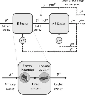
The two-sector model proposed in our own work – while inspired by the work of Ayres & Warr (2005; 2009) – differs from the latter effort in several aspects. In our description of the economy we look at overall production as a two-stage process, with a separation between energy-related activities, and the remaining economic production activities. Figure 2 illustrates the two-sector model for the economy considered in our analysis.
consumption goods and services in the economy. By isolating all energy conversion and transformation activities in an (abstract) extended energy sector, this model is in line with the
Warr & Ayres (2006) argument that a major driver of economic growth is “technical progress”, not as an exogenous residual, but rather as concentrated in historical improvements in primary-to-final-to-useful energy/exergy efficiency, which are entirely located in our proposed extended energy sector.
[image:15.612.169.460.238.555.2]It is assumed, throughout our analysis, that we are dealing with a closed economy, running in continuous time, and populated only by consumers (i.e. households, government, and NPISHxxi) and firms. Other components such as imports/exports, taxes and subsidies, as well as capital transfers and net lending/borrowing, are disregarded in our analysis. Markets are assumed to be perfectly competitive, in the sense that economic agents take prices as given.
Figure 2 – Two-sector model framework for the economy. Physical flows (e.g. primary/useful exergy) are represented as full lines. Monetary flows (e.g. consumption/investment expenditure) are represented as dashed lines.
consumption goods and services, 𝐶 (𝑡), and investment in physical capital, 𝐼(𝑡) = 𝐼 (𝑡) + 𝐼 (𝑡), to supply both economic sectors.
Production processes within the NE-Sector generate this sector’s total output, given by
𝑌 (𝑡)xxii. Unlike the model developed by Ayres & Warr (2005; 2009), the assumption that factors of production are used in the same proportions for the energy sector as for the whole economy – is lifted in our proposed two-sector framework.
The total product of the economic system illustrated in Figure 2 then corresponds to the sum of the NE-Sector production output and the monetary value attributed to final directly consumed useful exergy. This total product for the economy corresponds to gross domestic product (GDP). There are two different (standard) approaches to measuring GDP: the
production, or value-added approach; and the expenditure approach. The production approach sums the outputs from every class of enterprise and deducts intermediate consumption (the cost of material, supplies, and services used in production) from this value, in order to obtain GDP:
𝑌 = 𝑌 + (1 − 𝛾)𝑝 𝐵 ( 4)
The gross output for the whole economic system – as depicted in Figure 2 – is given by
𝑌 + 𝑝 𝐵 , in which 𝑝 corresponds to the price attributed to useful exergy output from the E-Sector. Hence, 𝛾𝑝 𝐵 represents the total monetary value associated with intermediate products used up in the production processes within the NE-Sector.
Alternatively, the expenditure approach measures GDP according to the total amount of money spent in the purchase of goods and services. For a closed economy such as our own, this translates as
𝑌 = 𝐶 + 𝐼 = 𝐶 + 𝐶 + 𝐼 + 𝐼 ( 5)
Both alternative approaches to measure GDP should, in principle, yield the same result. When applying the proposed model to empirical data, collected datasets will be decomposed and reclassified according to the variables defined in the expenditure approach, as presented in Equation 5.
The extended energy sector introduced in our work is innovatively defined, when compared to general economic models and accounts. The traditionally defined energy sector is generally associated exclusively with the energy industries, i.e. those involved in the production and sale of energy and energy related products, including fuel extraction, manufacturing, refining, and distribution activities. More specifically, the traditionally defined energy sector includes (Case & Fair, 2007):
The petroleum industry, including oil companies, petroleum refiners, fuel transport, and end-user sales at gas stations;
The gas industry, including natural gas extraction and coal gas manufacture, as well as distribution and sales;
The electrical power industry, including electricity generation and electric power distribution and sales;
The coal industry;
The renewable energy industry, comprising alternative energy and sustainable energy companies, including those involved in hydroelectric power, wind power, and solar power generation, and the manufacture, distribution, and sale of alternative fuels;
Traditional energy industry based on the collection and distribution of firewood, the use of which, for cooking and heating, is particularly common in poorer countries.
In the proposed two-sector model presented in our work, the extended energy sector is defined by boundaries that go beyond the traditional energy industries. Namely, this extended energy sector aggregates every single process involved in the conversion of primary energy (or exergy), extracted from the environment, into final energy (exergy) sold to consumers, and into useful exergy actually used to perform a final function in the economy. Hence, within the boundaries defined for our extended energy sector, lie not only the primary-to-final energy (exergy) transformation processes that compose the traditional energy industries, but also all final-to-useful exergy transformation processes that occur within any end-use device used in the economy. Concretely, this means that the extended energy sector includes not only machines used in the traditional energy industries (e.g. boilers and turbines used in a coal fired power plant), but also devices used in households and firms (e.g. refrigerators, laptops, automobiles, etc.). In this sense, the defined energy sector (E-Sector) is much broader than the traditional energy sector composed of energy industries only. This extended energy sector encompasses all processes of energy transformation and conversion in the economy, and its output corresponds to useful exergy actually used to perform economic activities and generate economic value.
The efficiency with which useful exergy is generated from primary exergy resources depends on efficiencies which are related with the technological capacity of the extended energy sector. In value terms, output for the extended energy sector (E-Sector) is given by
𝑌 = 𝑝 𝐵 = 𝐵 (6)
A constant positive fraction of the total useful exergy output from the extended energy sector 𝛾𝐵 will be consumed as a factor of production in the APF governing the production of goods and services in the non-energy sector. The remaining fraction (1 − 𝛾) 𝐵 will correspond to useful exergy directly consumed by households, government, and NPISH. In monetary terms, this is written as
𝑌 = 𝐶 + 𝛾𝐵
𝐶 = (1 − 𝛾)𝐵 ( 7)
The novel definition for an extended energy sector within our proposed two-sector framework for the economy implies a redefinition of variables pertaining to consumption and investment expenditure, as well as useful exergy use, by both sectors. In the next sections we propose a simplified first approach to conduct the decomposition and reclassification of expenditure and energy balances datasets according to the two-sector model’s variables as defined in our framework.
2.2.
Decomposition and reclassification of National Accounts
These accounts include detailed underlying measures relying on double-entry bookkeeping. National income and product accounts provide estimates for the value of income and output on an annual basis, including GDP. The expenditure approach focuses on estimating total output through measurement of the amount of money spent by economic agents. For a closed economy disregarding imports and exports:
𝐺𝐷𝑃 = 𝐶 + 𝐼 ( 8)
In Equation 8, 𝐶 corresponds to total final consumption expenditure – the sum of private expenditure by households and NPISH, and general government expenditure. The second r.h.s. term 𝐼 corresponds to gross private domestic investmentxxiii.
In our proposed two-sector model approach, consumption and investment expenditure for the whole economy can be decomposed as consumption and investment expenditure incurred by each of the two sectors. Hence, total consumption expenditure for the whole economy will correspond to the sum of consumption expenditure on goods and services produced in the non-energy sector (𝐶 ), and consumption of useful exergy output from the extended energy sector by households, firms, and NPISH (𝐶 ). Analogously, total investment expenditure will correspond to the sum of investment expenditure in physical capital used in NE-Sector production (𝐼 ), and physical capital used in E-Sector generation of useful exergy (𝐼 ).
Since the extended energy sector defined in our two-sector framework – as detailed in Section 2.1.1 – encompasses not only primary-to-final energy (exergy) conversion devices found in traditional energy industries, but also final-to-useful exergy conversion devices found in households; and since these latter devices (conventionally accounted as consumer goods) constitute an investment in the physical capital required by the extended energy sector to generate its output (useful exergy) from primary energy resources; it follows that adjustments have to be made when classifying investment expenditure in the extended energy sector.
Concretely, a redefinition of selected (those performing final-to-useful exergy conversion) traditionally-defined consumer goods, produced by the NE-Sector, as investment in physical capital in the extended energy sector is required in order to have a clear-cut separation between the two sectors. Because of this requirement, total consumption and investment expenditure for our proposed two-sector framework will necessarily differ from consumption and investment expenditure as reported in national accounts. Specifically, the redefinition of consumer goods as investment will result in lower values for total consumption expenditure – compared with national accounts – and correspondingly higher values for total investment expenditure. This can be expressed mathematically as
𝐶∗= 𝐶 + 𝐶 < 𝐶
𝐼∗ = 𝐼 + 𝐼 > 𝐼
𝐶∗+ 𝐼∗= 𝐶 + 𝐼 ( 9)
Where 𝐶 and 𝐼 correspond to total consumption and investment expenditure as defined in national accounts, respectively, and 𝐶∗ and 𝐼∗ corresponds to total consumption and
𝐺𝐷𝑃 = 𝐶∗+ 𝐼∗+ (𝑋 − 𝑀) ( 10)
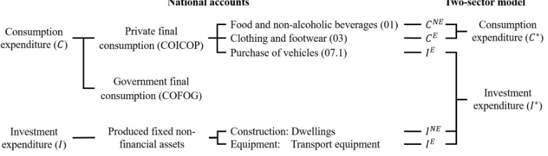
[image:19.612.110.502.224.336.2]The following sections deal – in detail – with the decomposition of national accounts total consumption expenditure 𝐶 and total investment expenditure 𝐼 according to final use and asset type, respectively. Each consumption and investment expenditure category is analyzed and allocated to the four disaggregate key variables associated to each sector’s consumption and investment expenditure, as defined in our framework (𝐶 , 𝐶 , 𝐼 , 𝐼 ). This allocation is performed following some simplifying criteria which should not, in principle, affect the general quality of results. A schematic depiction illustrating (through selected examples) the decomposition and reclassification effort detailed in the following sections is presented in Figure 3.
Figure 3 – Diagram representing the decomposition of standard macroeconomic national accounts (left) and reclassification according to the variables defined in the proposed two-sector model with an extended energy sector
(right). Consumption expenditure (e.g. private final consumption) is decomposed according to purpose and reclassified as either directly consumed useful exergy (𝐶 ), non-energy related consumption (𝐶 ), or investment in
the extended energy sector (𝐼 ). Investment expenditure is decomposed according to type of asset and reclassified as either investment in the non-energy (𝐼 ) or extended energy (𝐼 ) sectors. Total consumption and investment
expenditure in the proposed two-sector model then differs from national accounts as in Equation (10).
2.2.1. Total consumption expenditure
Total final consumption expenditure, as defined by macroeconomic national accounts, comprises both the expenditure on goods and services used for the direct satisfaction of individual needs (individual consumption), or collective needs of members of the community (collective consumption). Total final consumption expenditure therefore comprises;
Final consumption expenditure by households and NPISH (private final consumption expenditure);
Final consumption expenditure by general government.
The most important component of final consumption expenditure comes from households and includes all durable and non-durable consumer goods. Exception is made of purchases for own-construction or improvements of residential housing, which are instead treated as a component of gross capital formation. Private household consumption is composed of:
All goods and services purchased by households to satisfy everyday needs;
Households’ consumption of outputs produced by unincorporated enterprises owned by households;
Imputed rents for services of owner-occupied housing;
Payments to government units to obtain various kinds of licenses, permits, certificates, passports, etc.;
Explicit and imputed service charges on household uses of financial intermediation services provided by banks, insurance companies, etc.
The classification of individual consumption according to purpose (COICOP) is a reference classification published by the United Nations’ Statistics Division. It divides the purpose of individual consumption expenditures incurred by households, NPISH, and general government. The classification units are transactions. Three structure levels are defined in COICOP:
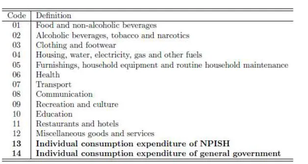
[image:20.612.155.469.268.435.2] Structure Level 1: Divisions (two-digit); Structure Level 2: Groups (three-digit); Structure Level 3: Classes (four-digit). The first structure level is presented in Table 1.
Table 1 – First COICOP structure level (divisions; two-digit) of private household consumption expenditure (1-12). Divisions 13 and 14 (bolded) represent individual consumption expenditure of non-profit institutions serving
households (NPISH) and of general government.
Divisions 01 through 12 are allocated to consumption expenditure incurred by households. Divisions 13 and 14 are allocated, respectively, to consumption expenditure incurred by NPISH and general government. For the purposes of the analysis conducted in our work, only Divisions 01 through 12 will be accounted as private final consumption expenditure (hence disregarding NPISH consumption expenditure), while general government consumption expenditure will be dealt with further ahead.
Both the INE and EUROSTAT macroeconomic databases provide detailed statistical data on the final consumption expenditure incurred by households disaggregated by COICOP divisions and groups, but not classes. For our analysis, this means that decomposition and aggregation of consumption expenditure datasets according to the variables defined in our proposed two-sector model framework will be conducted at the group level, risking some loss of precision in the obtained results.
constitutes consumption expenditure under the two-sector model’s definitions). In the latter case, the criteria adopted in our analysis consists of splitting the considered group/division in half and allocating each half with each of the two-sector model’s variables which match the group/division’s contents.
It is important to note that the redefinition of particular energy-driven consumption goods as investment in the extended energy sector (E-Sector) – the most innovative characteristic of our proposed two-sector model for the economic production – carries some concerns regarding the consistency in accounting consumption and investment expenditure for each sector. The concept of imputed rents applies to any capital goodxxiv and it must be taken into account when redefining automobiles and appliances, for example, as components of investment expenditure in the extended energy sector productive processes. The full cost of using a fixed asset in production is also measured by the actual or imputed rental on the asset, and not by depreciation alone. Although imputed rents are not explicitly accounted for in our work for each consumer good redefined as investment expenditure in the extended energy sector, it is expected that the effect of these imputed rents is eventually indirectly accounted for when estimating consumption of fixed capital for sector specific investment expenditure in the proposed two-sector model.
Final consumption expenditure incurred by households includes expenditure on services such as electricity, gas, and heat supply. These and other similar expenditures (such as the purchase of fossil fuels) are interpreted in our work as payments for the energy (i.e. exergy) contained within these products, and indirectly, for the useful exergy provided by this exergy content. Hence, the COICOP groups Electricity, gas and other fuels (04.5) and Operation of personal transport equipment (07.2) (which includes some expenditure on fuels) are allocated to direct useful exergy consumption by households 𝐶 ( ). The first two COICOP divisions –
Food and non-alcoholic beverages (01); Alcoholic beverages, tobacco and narcotics (02) – are also straightforwardly allocated to with 𝐶 ( ), for similar reasoning. These divisions concern
payments for food products, which can ultimately be equated with payments for the useful exergy (i.e. muscle work) extracted from the consumption of these food products. It is then assumed that all exergy contained in food products is to be converted to muscle work.
Due to the innovative definition adopted in our work concerning the extended energy sector, all consumption goods participating in the conversion of final energy/exergy to useful exergy are allocated not to consumption expenditure, but to investment expenditure in the extended energy sector (E-Sector) 𝐼 ( ). In practice, this means that consumption goods such
as motorized vehicles and electric appliances will be considered capital investment expenditure in our proposed two-sector model. The groups Purchase of vehicles (07.1) and
Telephone and telefax equipment (08.2) are the only ones allocated to 𝐼 ( ) in their entirety.
Both groups also include components accounting for expenditure in the repair of equipment, but such components are deemed negligible.
Most of the remaining individual COICOP groups and divisions can be allocated in its entirety to consumption expenditure by households on goods and services generated by the non-energy sector (NE-Sector) 𝐶 ( ). This is the case for Education (10), Restaurants and
and allocated to 𝐶 ( ) and 𝐼 ( ). One example is the COICOP group Audio-visual,
photographic and information processing equipment (09.1), which includes both physical capital responsible for the conversion of final energy/exergy into useful exergy for other electrical uses (television sets, stereo systems, personal computers, etc.), as well as non-energy related consumption goods (compact disks, lenses, software, etc.). For these cases, the datasets are equally split between the two key variables. A similar methodology will be applied for the decomposition and aggregation of final consumption expenditure of general government categories (COFOG).
Final consumption expenditure of general government consists of expenditure incurred by government in its production of non-market final goods and servicesxxv and market goods and services provided as social transfers in kind. Included in the final consumption expenditure of general government are:
Non-market output other than own-account capital formation, which is measured by production costs less incidental sales of governmental output;
Expenditure on market goods and services that are supplied without transformation and free of charge to households (social transfers in kind).
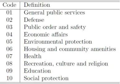
[image:22.612.210.404.419.555.2]Analogously to private final consumption expenditure, the United Nations’ Statistics Division classifies government expenditure datasets in national accounts according to the purpose for which the funds are used. This is done through the classification of the functions of government (COFOG), which allocates government expenditure for specific uses. It corresponds to the 14th division in the COICOP classification, and exhibits a similar structure level, with transactions as units. The COFOG divisions are presented in Table 2.
Table 2 – First COFOG structure level (divisions; two-digit) of government consumption expenditure.
The first 3 COFOG divisions – General public services (01); Defense (02); Public order and safety (03) - plus Environmental protection (05), Education (09), and Social protection (10), can be entirely allocated to the two-sector variable 𝐶 ( ), along with the majority of the
remaining COFOG groups. Exceptions are the COFOG groups Transport (04.5), Communication (04.6), Street lighting (06.4), and Medical products, appliances, and equipment (07.1), all of which including elements allocated to different key variables of the proposed two-sector model. For these latter COFOG groups, annual values are split in half and allocated equally to the two-sector variables 𝐶 ( ) and 𝐼 ( ). The COFOG group Fuel and energy (04.3) is entirely
allocated to direct consumption of useful exergy by the government 𝐶 ( ). As before, it is
Total final consumption expenditure in macroeconomic national accounts corresponds to the sum of private final consumption expenditure and general government consumption expenditure. The sum of aggregate two-sector model’s variables corresponding to the consumption of non-energy related (NE-Sector produced) goods and services by households and government – 𝐶 ( ) and 𝐶 ( ) respectively – with the direct consumption of useful
exergy by households and government – 𝐶 ( ) and 𝐶 ( ), respectively – constitutes total final
consumption expenditure under the definitions adopted for the proposed two-sector model framework:
𝐶 = 𝐶 + 𝐶 = 𝐶 ( )+ 𝐶 ( )+ 𝐶 ( )+ 𝐶 ( ) ( 11)
2.2.2. Total investment expenditure
Gross capital formation in macroeconomic national accounts represents investment expenditure in capital assets. Gross capital formation incorporates not only produced capital goods (e.g. machinery, buildings, roads) but also improvements to non-produced assets. Hence, gross capital formation (GCF) constitutes a measure for the additions to the capital stock of buildings, equipment, and inventories – i.e. the addition to the capacity of the economy to produce more goods and income in the future. The components of GCF can be listed as:
Gross fixed capital formation (GFCF); Changes in inventories;
Acquisition less disposals of valuables.
For the purposes of the analysis presented in our work, only the major components of GCF – i.e. gross fixed capital formation (GFCF) – will be considered for the computation of investment expenditure. This component of GCF incorporates (Schreyer, 2009):
Acquisition less disposal of new or existing produced assets, such as dwellings, other building structures, machinery and equipment, cultivated assets (e.g. trees and livestock), mineral exploration, computer software, entertainment, literary or artistic originals, and other intangible fixed assets;
Costs of ownership transfers on non-produced, non-financial assets, such as land and patented assets;
Major improvements to produced and non-produced, non-financial assets that extend the lives of assets;
Acquisition that can be in terms of purchase, own-account production, barter, capital transfer in kind, financial leasing, natural growth of cultivated assets and major repairs of produced assets;
production. Hence, an automobile purchased for personal use does not constitute GFCF but is rather accounted for as final consumption expenditure of households – Table 4. However, under the innovative definition of variables according to the two-sector modelling framework proposed in our work, automobiles constitute capital assets actively participating in the conversion of final energy/exergy to useful exergy, and therefore constitute investment expenditure in the extended energy sector (E-Sector) of the economy, regardless of being used in economic productive processes or leisure.
Non-produced assets such as land, mineral reserves, and natural resources (water, primary forests, etc.), as well as repair work and purchases of household durable equipment, are excluded from official measures for GFCF. In relevant literature and databases, detailed breakdowns of GFCF are available according to:
Type of asset (plant, machinery, land improvements, buildings, vehicles, etc.); Industry (manufacturing, construction, services, etc.);
Economic sector (residential versus non-residential, government sector versus private sector, market sector versus non-market sector, etc.).
[image:24.612.145.482.339.639.2]According to the definitions provided by the European System of Accounts (ESA 95), only produced fixed non-financial assets constitute GFCF – Figure 4.
Figure 4 – Classification of fixed assets according to the European System of Accounts (ESA95). Breakdown of non-financial produced fixed assets by type of asset.
two-sector model’s variables concerning investment expenditure in the extended energy two-sector (E-Sector) 𝐼 ( ), and in the non-energy sector (NE-Sector) 𝐼 ( ). Total investment expenditure in
the extended energy sector’s production processes 𝐼 is equivalent to the sum of consumption expenditure components redefined as investment in this sector – 𝐼 ( ) and 𝐼 ( ) – and 𝐼 ( ).
The GFCF asset categories for construction are entirely allocated to investment expenditure in the non-energy sector production processes 𝐼 ( ) – Table 8. The bulk of the
dwellings category refers to buildings and structures used for residence. Some types of residences included in this category, such as mobile homes and caravans, could be considered as investment expenditure in the extended energy sector 𝐼 ( ), due to their participation in
the conversion of final energy/exergy to useful exergy. However, these components of the dwellings category in GFCF are considered negligible. The non-residential construction and civil engineering GFCF category concerns warehouse, industrial and commercial buildings, mostly. Other structures such as roads, streets, tunnels, harbors, and airfield runways are also included in this category. For the analysis in our work, the category Other Investment is split in half and each fraction allocated to E-Sector and NE-Sector investment expenditure. Cultivated assets include livestock for breeding, dairy, draught, vineyards, orchards, and other plantations of trees yielding repeat products. Intangible fixed assets consist mainly of mineral exploration, computer software, entertainment and literary/artistic originals. The former constitute investment in the extended energy sector, while the latter constitute investment in the non-energy sector production processes.
Transport equipment is entirely allocated to investment expenditure in the extended energy sector 𝐼 ( ). This GFCF category includes motor vehicles, motorcycles, railways and
tramway locomotives, and aircrafts, all of which participate in the conversion of final energy/exergy to useful exergy – namely in the form of mechanical drive.
The GFCF category for metal products and machinery includes assets that participate in the conversion from final energy/exergy to useful exergy (e.g. office machinery, communication equipment, agricultural machinery, etc.) and also assets which constitute investment expenditure in the NE-Sector. Analogous to the assumptions adopted earlier for COICOP and COFOG categories for consumption expenditure, this asset category is equally split between 𝐼 ( ) and 𝐼 ( ).
The fraction of GFCF allocated to investment expenditure in the NE-Sector constitutes the entirety of investment expenditure in this sector of the proposed two-sector model: 𝐼 = 𝐼 ( ). Investment expenditure in the extended energy sector is equal to the sum of the
fraction of GFCF allocated to this sector’s investment expenditure 𝐼 ( ), and the consumption
expenditure categories redefined as investment expenditure in this sector – 𝐼 ( )+ 𝐼 ( ).
Total investment expenditure for both sectors of the proposed two-sector model is then
𝐼 = 𝐼 + 𝐼 = 𝐼 ( )+ 𝐼 ( )+ 𝐼 ( )+ 𝐼 ( ) ( 12)
2.2.3. Capital stock and depreciation
In order to accurately estimate annual time series for capital stock (𝐾) pertaining to each of the sectors in the proposed two-sector model for the economy – 𝐾 and 𝐾 – it is first necessary to take into account the depreciation of capital assets, which requires determining the annual datasets for the consumption of fixed capital (𝐶𝐹𝐶) in each sector – 𝐶𝐹𝐶 and
𝐾 (1960). The respective annual capital stock datasets for each sector are then computed through a perpetual inventory methodxxviii:
𝐾 (𝑡 + 1) = 𝐾 (𝑡) − 𝐶𝐹𝐶 (𝑡) + 𝐼 (𝑡)
𝐾 (𝑡 + 1) = 𝐾 (𝑡) − 𝐶𝐹𝐶 (𝑡) + 𝐼 (𝑡) ( 13)
Consumption of fixed capital (CFC) is a term used in business and national accounts to measure the amount of fixed capital that is used up, each year, in the process of generating new output. The measurement CFC may also incorporate – beyond actual depreciation charges – expenses incurred in using or installing fixed assets. Through simple association, CFC datasets corresponding to investment expenditure in each of the two sectors considered in our proposed economic model is estimated as:
𝐶𝐹𝐶 = × 𝐶𝐹𝐶
𝐶𝐹𝐶 = × 𝐶𝐹𝐶 ( 14)
Initial values for capital stock datasets concerning each of the two sectors – 𝐾 (1960)
and 𝐾 (1960) – are determined also by simple association, from data on total capital stock 𝐾,
𝐺𝐹𝐶𝐹, and 𝐶𝐹𝐶. Initial values for capital stock in the extended energy sector (E-Sector) and NE-Sector are hence given by:
𝐾 (1960) =
( )
( )× 𝐾(1960)
𝐾 (1960) = (( ))× 𝐾(1960) ( 15)
Annual datasets for capital stock in both sectors of the proposed economic model – 𝐾
and 𝐾 – are computed through the perpetual inventory method presented in Equation 13. Total annual capital datasets (𝐾) are computed as the sum of 𝐾 and 𝐾 annual datasets.
2.3.
Decomposition and reclassification of useful exergy balances
Besides the decomposition and reclassification of macroeconomic variables, an analogous decomposition and reclassification for useful exergy used in NE-Sector production, or directly by consumers, is also required for a detailed and accurate depiction of economic production within our two-sector framework. Namely, annual values must be assigned to primary exergy from natural resource inputs to the extended energy sector’s productive processes – 𝐵 –, as well as to useful exergy consumed directly by households – 𝛾𝐵 –, and useful exergy used by the productive processes of the non-energy sector – (1 − 𝛾)𝐵 . The values for these variables can be computed from the analysis of energy balances from mainstream databases, in combination with alternative sources of data, and the application of the methodology developed in Serrenho et al. (2016).
2.3.1. Decomposition of energy consumption
Decomposition of energy consumed by the economy’s productive processes begins at country-level energy balances, discriminating between primary energy supply (𝐸 ), gross energy consumption, energy industry own-uses, and final energy consumption. For an accurate and detailed decomposition and reclassification of energy balances according to the two sectors of the proposed economic model – as well as its conversion to useful exergy figures (see
heat; food and feed for humans and working animals; other non-conventional carriers, including for example wind kinetic energy), and by institutional sector (industry; transport; other, including residential; non-energy uses; and energy industries own-uses).
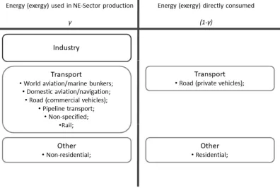
[image:27.612.106.502.223.489.2]By analyzing a country’s energy balances, and their respective decomposition by institutional sector (and further subdivisions), it is possible to obtain estimates for the total final energy (minus energy industries own-uses) that is directly consumed by households and governments – corresponding to the fraction (1 − 𝛾) – and that which is used in production processes within the NE-sector – corresponding to the fraction 𝛾. The decomposition and aggregation of energy balances under the corresponding two-sector variables is illustrated in Figure 5.
Figure 5 – Disaggregation and reclassification of total final exergy consumption (minus energy industries own-uses) according to direct consumption by households and government, and production processes within the Non-energy
Sector.
According to our decomposition and aggregation of energy balances, all final energy (exergy) consumed by the Industry sector of the economy will generate useful exergy to be applied in NE-sector production processes. Likewise, the majority of subdivisions in Transport
and Other institutional sectors are also directly allocated to the generation of useful exergy for NE-Sector production processes. Exceptions are the Transport subdivision of Road – which includes fuels consumed by both private and commercial vehicles – and the Other subdivision of Residential – which corresponds to the energy consumed in households. Regarding the Road
![Figure 1 – Generalized positive feedback cycle. [Source: Warr & Ayres, 2006]](https://thumb-us.123doks.com/thumbv2/123dok_us/180050.514876/8.612.155.454.299.526/figure-generalized-positive-feedback-cycle-source-warr-ayres.webp)