N dimensional probability density function transfer and its aplication to colour transfer

N-Dimensional Probability Density Function Transfer

and its Application to Colour Transfer

Franc¸ois Piti´e , Anil C. Kokaram and Rozenn Dahyot

University of Dublin, Trinity College

Dublin 2, Ireland

[email protected]

Abstract

This article proposes an original method to estimate a continuous transformation that maps one N-dimensional distribution to another. The method is iterative, non-linear, and is shown to converge. Only 1D marginal distribu-tions are used in the estimation process, hence involving low computation costs. As an illustration this mapping is applied to colour transfer between two images of different contents. The paper also serves as a central focal point for collecting together the research activity in this area and relating it to the important problem of Automated Colour Grading.

1. Introduction

The principle of example-based rendering is probably the simplest and most effective approach to rendering real-istic images. The idea is to transfer the statreal-istics of a target dataset (the example) to a source dataset. After transfer, the re-rendered source dataset has the same look and feel as the target one. The recent breakthrough in texture synthesis [4] is probably one of the most significant examples of this idea. By simply sampling from the neighbouring distribution of a seed example texture, it is possible to synthesise bigger pictures that look similar. The success of realistic rendering thus relies on the transfer of real data statistics.

The idea of transfer of statistics encompasses an entire range of possibilities from the simple match of the mean and variances of both datasets to the exact transfer of the whole probability density function (pdf) of the samples. This pa-per considers the general problem of finding a continuous mapping that transforms the source samples into a new en-semble of samples that exhibits the same pdf as the target samples. Finding a mapping for one-dimensional (1D) sam-ples is a simple task that can be solved in the same way as grayscale picture equalisation [5]. The difficulty resides in

extending the method to higher dimensions.

There are a wide range of applications for the notion of exact transfer of pdf’s for multidimensional datasets. In the transfer of colour between two images, it is known as exampled-based colour transfer [14]. In digital restora-tion [12] the idea is to recolour paintings that have been faded by smoke, dust etc. If the target pdf is uniform, the process can also be used for colour image equalisation for scientific data visualisation [13] or simply used for non-realistic rendering. In particular, a major problem in the post production industry is matching the colour between different shots possibly taken at different times in the day. This process is part of the large activity offilm gradingin which the film material is digitally manipulated to have con-sistent grain and colour. The termcolour gradingwill be used specifically to refer to the matching of colour. Colour grading is important because shots taken at different times under natural light can have a substantially different ‘feel’ due to even slight changes in lighting. Currently these are fixed by experienced artists who manually tune parameters. This is a delicate task and the method presented in this pa-per succeeds in automating this painstaking process even when the lighting conditions have dramatically changed, as shown in figure 4.

2. Related Work

Transfer of Colour Statistics. One popular method [14] matches the mean and variance of the target image to the source image. The transfer of statistics is performed sep-arately on each channel. Since the RGB colour space is highly correlated, the transfer is done in the less correlative colour spacelαβ which has been proposed to account for human-perception [15]. But the method is limited to linear transformations and some example-based recolouring sce-narios actually require non-linear colour mapping. Figure 1 shows exactly this problem and the method fails to transfer any useful statistics.

The problem of finding a non-linear colour mapping is addressed in [13] for colour equalisation (like for grayscale histogram equalisation). The paper proposes to deform the tessellation meshes in the colour space to fit to the 3D his-togram of uniform distribution. This method can be seen as being related to warping theory which is explicitly used in [10] where the transfer of the 2D chromatic space is per-formed directly by using a 2D-biquadratic warping.

Without having to invoke image warping, an extension of the 1D case is to find the mapping via linear program-ming [11] and the popular Earth-Mover distance. The ma-jor disadvantage of the method is that 1) the mapping is not continuous and 2) pixels of same colours may be mapped to pixels of different colours, which require random selection. Furthermore the computational cost becomes intractable if a very fine clustering of the colour space is desired.

Dealing with Content Variations. One important aspect of the colour transfer problem is the change of content be-tween the two pictures. For example the target picture may present more sky than the source picture. Since all colour transfer algorithms are sensitive to the variations of the colour cluster sizes, they risk overstretching the colour mappings and thus producing unbelievable renderings.

To deal with this issue a simple solution [14] is to man-ually select swatches in both pictures and thus associate colour clusters corresponding to the same content.

One automated solution is to invoke the spatial informa-tion of the images to constrain the colour mapping [7]. The extreme case is colouring grayscale pictures. Retrieving the missing chrominance channels values can be done by taking advantage of similarities between spatial neighbourhoods of the two pictures [16, 6].

Another automated method is to restrict the variability on the colour mapping. For example in [1], the pixels of both images are classified in a restricted set of basic colour categories, derived from psycho-physiological studies (red, blue, pink. . . ). The colour transfer ensures that blue-ish pix-els remain blue-ish pixpix-els. This gives a more natural trans-formation but limits the range of possible colour transfers.

target image original image Reinhard

Figure 1. Example of Colour transfer using Reinhard [14] Colour Transfer. The transfer fails to resynthesise the colour scheme of the target image. To be successful the method would require human interaction.

By contrast our method is able to map shades of green to shades of orange in the first row of figure 4.

Novelty. The work presented in this paper addresses many of the shortcomings of previous efforts in this area. Firstly, it is computationally attractive as it uses just 1D pdf match-ing in an iterative scheme which is shown to converge. Sec-ondly, the method is completely non-parametric and is very effective at matching arbitrary distributions. The paper also serves as a central focal point for collecting together the re-search activity in this area and relating it to the important problem of Automated Colour Grading which has not been previously specifically addressed in this community.

3. N-Dimensional pdf Transfer

Denotef(x) and g(y) the pdf of X and Y, the orig-inal and targetN-dimensional continuous Random Vari-ables respectively. For example in colour transfer, the samplesx_iofX encapsulate the three colour components

x_i = (r_i, g_i, b_i). The goal is to find a continuous mapping functiontthat transformsfing.

Dimension N = 1. This is a well known problem [5] which offers a simple solution:

t(x) =C−1

Y (CX(x)) (1)

whereC_XandC_Yare the cumulative pdfs ofXandY. This can be easily solved using discrete lookup tables.

Algorithm 1pdf transfer algorithm

1: Initialisationof the data set sourcexand targety. For example in colour transfer,x_j= (r_j, g_j, b_j)wherer_j, g_j, b_jare the red, green and blue components of pixel numberj.

k←0, x(0)_←x

2: repeat

3: take a rotation matrixRand rotate the samples:xr←Rx(k)andyr←Ry

4: project the samples on all axisito get the marginalsf_iandg_i

5: for each axisi, find the 1D transformationt_ithat matches the marginalsf_iintog_i

6: remap the samplesx_raccording to the 1D transformations. For example, a sample(x₁, . . . , x_N)is remapped into

(t₁(x₁), . . . , t_N(x_N)), whereNis the dimension of the samples.

7: rotate back the samples:x(k+1)←R−1x_r 8: k←k+ 1

9: untilconvergence on all marginals for every possible rotation 10: The final one-to-one mappingtis given by:∀j ,xj→t(xj) =x(∞)j

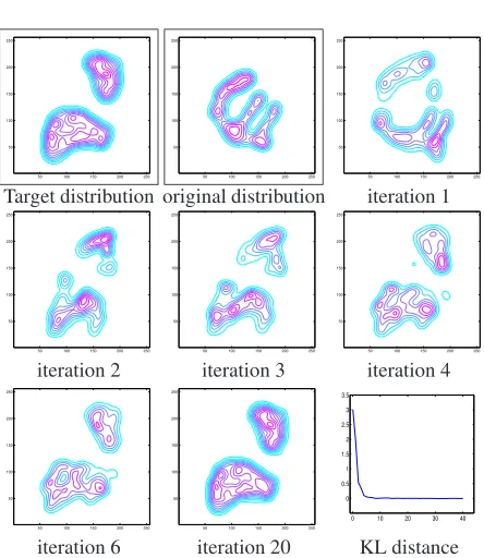
samples is proved to be actually closer to the target distri-bution than before transformation. The main point of this paper is to observe that iterating this simple procedure for different set of axes is sufficient to eventually transform the original samples into a distribution that is identical to the target distribution.

The algorithm operates as follow. At iterationk, the sam-ples involved are the iterated samsam-ples of X(k) (the trans-formed image) and the samples fromY (the target image). The first step of the iteration is to change the coordinate sys-tem by rotatingboththe samples ofX(k) and the samples ofY. In a second step the samples of both distributions are projected on the new axes which gives the marginals

f₁. . . f_N andg₁. . . g_N. Then it is possible using equation

(1) to find for each axisithe mappingst_i:∀j x_j→t_i(x_j) that transfers the marginals fromf_itog_irespectively. The resulting transformationtmaps a sample(x₁, . . . , x_N)into

t(x₁, . . . , x_N) = (t₁(x₁), . . . , t_N(x_N)). The iteration is

completed with a rotation of the samples byR−1to return in the original coordinate system.

The iteration leaves the samples fromgunchanged and transforms the pdff(k)intof(k+1). The algorithm is shown to converge tof(∞) = g if the operation is repeated for enough different rotations (taking random rotations is suf-ficient to converge). The full algorithm in presented in a separate figure on this page and is simple to implement as it requires no extra parameters.

The outline of the method presents some resemblance with an iterative algorithm of gaussianization of data pre-sented in [9]. However this method investigates a much wider range of transformations as it proposes to match not only gaussians distributions but any kind of distribution. Moreover a mathematical proof of the method is presented, whereas in [9] the validity of the method is limited to nu-merical experiments.

50 100 150 200 250 50

100 150 200 250

50 100 150 200 250 50

100 150 200 250

50 100 150 200 250 50

100 150 200 250

Target distribution original distribution iteration 1

50 100 150 200 250 50

100 150 200 250

50 100 150 200 250 50

100 150 200 250

50 100 150 200 250 50

100 150 200 250

iteration 2 iteration 3 iteration 4

50 100 150 200 250 50

100 150 200 250

50 100 150 200 250 50

100 150 200 250

0 10 20 30 40 0 0.5 1 1.5 2 2.5 3 3.5

iteration 6 iteration 20 KL distance

Figure 2. Example of 2D pdf transfer. Note the decrease of the measure of the Kullback-Leibler distance.

mapping function get closer to the identity mapping ifm increases. Such a modification slows down the convergence of the algorithm but it is often required since the content of the pictures rarely match exactly.

4. Proof of the Method

Proof. Consider the operationT which describes one itera-tion of our algorithm (ie, rotate, transform and rotate back the samples): the target distributiongis of course station-ary forT sinceT(Y) =Y andT transformsf(k)inf(k+1) withX(k+1)=TX(k).

The Data Processing Theorem [8, pp. 18-22] — which is fundamental in Information Theory — states that no statisti-cal processing of the data can increase the Kullback-Leibler distance. Thus the Kullback-Leibler distance betweenf(k) andgdecreases for each iterationk, and this for every pos-sible rotation and initial distributions.

Df(k)_g≥DTf(k)_{T(g) (2)}

Df(k)_g≥Df(k+1)_{g (3)}

The sequence Df(k)g is monotonically non-increasing non-negative and must therefore have a limit. The limit is actually 0 if the stationary distribution g is unique (see [3, pp. 33-35]). It is then sufficient to prove that g is the unique stationary distribution to show the convergence of the sequencef(k)tof(∞)=g.

This can be done by invoking a geometrical argument. Lethbe another stationary distribution. By definition of the algorithm, for every rotation of the axis, the projections (or marginals) ofh match the projections ofg. Thus the

N-dimensional Radon Transforms ofhandgare identical. Since the Radon transform admits a unique inverse, we have

h=gand thusgis the only stationary distribution.

Numerical Experiences. The measure of the KL distance is performed via the kernel density approximation of the density. We implemented a kernel density estimation with variable bandwidth to account for the sparseness of sam-ples. A clear outline of the bandwidth selection is available in [2]. The numerical Kullback-Leibler distance or relative entropy can be computed as follow:

DKL(f g) = _N1

i

ln  

jK

xi−xj

h

jK

xi−yj

h

  (4)

whereKis the Epanechnikov kernel. As expected by the theory, the KL distance decreases with the iterationn(see figure 2).

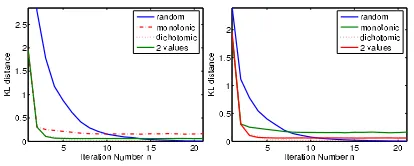
Figure 3. Convergence rate depending on the rotation selection strategy. If the random strategy (in solid blue) performs poorly in the first iterations it eventually outperforms our deterministic strategies.

Choice of the Rotation Matrices. From the proof we can state that the algorithm has to take marginals for every pos-sible rotation, where there is an infinite number of pospos-sible rotations. The simplest way of addressing this is to spread the angle values over the whole angular spectrum and sam-ple the angles of the rotation matrix from a uniform distrib-ution.

The convergence rate of the random selection strategy has been tested against 3 deterministic strategies. The first strategy is a monotonic increase of the rotation angles, the second strategy is a ping-pong between two fixed rotations (0 andπ/4) and the third strategy explores angles in a di-chotomous way (0,π/4, 0,π/8,π/4, 0,π/16,2π/16. . . ). The third method tries to emphasise the harmonics of the angular spectrum. Figure 3 shows that, on average over 50 experiences, the random sampling of rotation outper-forms eventually the deterministic schemes. In particular the monotonic scheme seems almost to stall.

5. Application to Image Recolouring

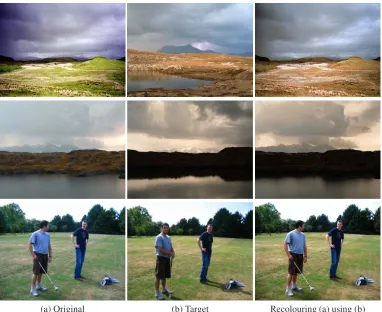
The last two pages show some results from the colour transfer technique proposed in the paper. Figure 4 displays some examples of colour transfer. For instance the origi-nal Alpine mountain picture in (b) is used as a target colour scheme for the Scottish landscape image in (a) the first col-umn. The result of the transfer appears in the last colcol-umn. The figure presents also examples of Colour Transfer for matching lighting conditions. On the second row, the colour properties of the sunset are used to synthesise the ‘evening’ scene depicted at sunset. On the last row, the colour trans-fer allows correction of the change of lighting conditions induced by clouds. A unavoidable limitation of colour grad-ing is the clippgrad-ing of the colour data: saturated areas cannot be retrieved (for instance the sky on the golf image can-not be recovered). A general rule is to match pictures from higher to lower range dynamics.

faded movies. The idea is similar to colour grading as we want to recreate different atmospheres. The target pictures used for recreating the atmosphere are on the second row.

6. Conclusion

This paper has proposed an original algorithm for trans-ferringN-dimensional pdfs. The method is guaranteed to converge at low computation costs. We have shown the ef-ficiency of the algorithm for colour transfer. Future works will look at its application to other areas of computer vision involving pdfs matching.

Acknowledgements

The authors would like to acknowledge the helpful discussions with Bill Collis at The FoundryR_{. This}

work was supported in part by HEA Project TRIP and GreenParrotPicturesR_.

References

[1] Y. Chang, K. Uchikawa, and S. Saito. Example-based color stylization based on categorical perception. InProceedings of the 1st Symposium on Applied perception in graphics and visualization (APGV), pages 91–98. ACM Press, 2004. [2] D. Comaniciu, V. Ramesh, and P. Meer. The Variable

Band-width Mean Shift and Data-Driven Scale Selection. InIEEE Int. Conf. Computer Vision (ICCV’01), pages 438–445, Van-couver, Canada, 2001.

[3] T.M. Cover and J.A. Thomas. Elements of Information The-ory. Wiley, 1991.

[4] A. A. Efros and T. K. Leung. Texture synthesis by non-parametric sampling. InIEEE International Conference on Computer Vision, pages 1033–1038, Corfu, Greece, Septem-ber 1999.

[5] R. C. Gonzalez and R. E. Woods.Digital Image Processing. Addison Wesley, 1992.

[6] Y. Ji, H-B. Liu, X-K Wang, and Y-Y. Tang. Color Transfer to Greyscale Images using Texture Spectrum. InProceedings of the Third International Conference on Machine Learning and Cybernetics, Shanghai, 2004.

[7] J. Jia, J. Sun, C-K. Tang, and H-Y. Shum. Bayesian correc-tion of image intensity with spatial consideracorrec-tion. In Euro-pean Conference on Computer Vision (ECCV), 2004.

[8] S. Kullback. Information Theory and Statistics. Wiley, New York, 1959.

[9] J.-J. Lin, N. Saito, and R. A. Levine. An iterative non-linear Gaussianization algorithm for resampling dependent components. InProc. 2nd International Workshop on Inde-pendent Component Analysis and Blind Signal Separation, pages 245–250, 2000.

[10] L. Lucchese and S. K. Mitra. a new Method for Color Image Equalization. InIEEE International Conference on Image Processing (ICIP’01), 2001.

[11] J. Morovic and P-L. Sun. Accurate 3d image colour histogram transformation. Pattern Recognition Letters, 24(11):1725–1735, 2003.

[12] M. Pappas and I. Pitas. Digital Color Restoration of Old Paintings. Transactions on Image Processing, (2):291–294, Feb. 2000.

[13] E. Pichon, M. Niethammer, and G. Sapiro. Color histogram equalization through mesh deformation. InIEEE Interna-tional Conference on Image Processing (ICIP’04), 2003.

[14] E. Reinhard, M. Ashikhmin, B. Gooch, and P. Shirley. Color transfer between images. IEEE Computer Graphics Appli-cations, 21(5):34–41, 2001.

[15] D.L. Ruderman, T.W. Cronin, and C.C. Chiao. Statistics of Cone Responses to Natural Images: Implications for Visual Coding.Journal of the Optical Society of America, (8):2036– 2045, 1998.

(a) Original (b) Target Recolouring (a) using (b)

Figure 4. Examples of Colour Transfer. On the first row the Scottish landscape is recoloured to match the palette of the Alpine scenery. On the second row, the colour properties of the sunset are used to synthesise the ‘evening’ scene depicted at sunset. On the third row, the colour transfer allows to correct the change of lighting conditions induced by clouds.

Original Frame 70’s atmosphere pub atmosphere