Proceedings of VarDial, pages 42–53 42
Modeling Global Syntactic Variation in English
Using Dialect Classification
Jonathan Dunn University of Canterbury Department of Linguistics
Abstract
This paper evaluates global-scale dialect iden-tification for 14 national varieties of English as a means for studying syntactic variation. The paper makes three main contributions: (i) in-troducing data-driven language mapping as a method for selecting the inventory of national varieties to include in the task; (ii) producing a large and dynamic set of syntactic features us-ing grammar induction rather than focusus-ing on a few hand-selected features such as function words; and (iii) comparing models across both web corpora and social media corpora in order to measure the robustness of syntactic varia-tion across registers.
1 Syntactic Variation Around the World
This paper combines grammar induction (Dunn, 2018a, 2018b, 2019) and text classification (Joachims, 1998) to model syntactic variation across national varieties of English. This classification-based approach is situated within the task of dialect identification (Section 2) and eval-uated against other baselines for the task (Sections 7 and 8). But the focus is modelling syntactic variation on a global-scale using corpus data. On the one hand, the problem is to use a model of syntactic preferences to predict an author’s dialect membership (Dunn, 2018c). On the other hand, the problem is to take a spatially-generic gram-mar of English that is itself learned from raw text (c.f., Zeman, et al., 2017; Zeman, et al., 2018) and adapt that grammar using dialect identification as an optimization task: which constructions are more likely to occur in a specific regional variety? Because we want a complete global-scale model, we first have to ask: how many national va-rieties of English are there? This question, consid-ered in Sections 3 and 4, is essential for determin-ing the inventory of regional varieties that need to be included in the dialect identification task. This
paper uses data-driven language mapping to find out where English is consistently used, given web data and Twitter data, in order to avoid the arbi-trary selection of dialect areas. This is important for ensuring that each construction in the grammar receives the best regional weighting.
What syntactic features are needed to represent variation in English? As discussed in Section 6, this paper uses grammar induction on a large back-ground corpus to provide a replicable and dynamic feature space in order to avoid arbitrary limitations (e.g., lists of function words). The other side of this problem is to optimize grammar induction for regional dialects by using an identification task to learn regional weights for each part of the gram-mar: how much does a single generic grammar of English vary across dialects? To what degree does it represent a single dominant dialect?
Finally, a corpus-based approach to variation is restricted to the specific domains or registers that are present in the corpus. To what degree is such a model of variation limited to a specific register? This paper uses both web-crawled corpora and so-cial media corpora to explore the robustness of di-alect models across domains (Section 8). Along these same lines, how robust is a model of syn-tactic variation to the presence of a few highly predictive features? This paper uses unmasking, a method from authorship verification (Koppel, et al., 2007), to evaluate the stability of dialect mod-els over rounds of feature pruning (Section 9).
2 Previous Work
En-glish within so-called inner-circle varieties (for example, Labov, et al., 2016; Strelluf, 2016; Schreier, 2016; Clark & Watson, 2016). This paper joins recent work in taking a global ap-proach by using geo-referenced texts to represent national varieties (e.g., Dunn, 2018c; Tamaredo, 2018; Calle-Martin & Romero-Barranco, 2017; Szmrecsanyi, et al., 2016; Sanders, 2010, 2007; c.f., Davies & Fuchs, 2015). For example, this study of dialect classification containsinner-circle (Australia, Canada, United Kingdom, Ireland, New Zealand, United States), outer-circle(India, Malaysia, Nigeria, Philippines, Pakistan, South Africa), and expanding-circle (Switzerland, Por-tugual) varieties together in a single model.
The problem is that these more recent ap-proaches, while they consider more varieties of English, have arbitrarily limited the scope of vari-ation by focusing on a relatively small number of features (Grafmiller & Szmrecsanyi, 2018; Kruger & van Rooy, 2018; Schilk & Schaub, 2016; Collins, 2012). In practical terms, such work uses a smaller range of syntactic representations than comparable work in authorship analysis (c.f., Grieve, 2007; Hirst & Feiguina, 2007; Argamon & Koppel, 2013).
From a different perspective, we could view the modelling of dialectal variation as a classifi-cation task with the goal of predicting which di-alect a sample belongs to. Previous work has draw on many representations that either directly or in-directly capture syntactic patterns (Gamallo, et al., 2016; Barbaresi, 2018; Kreutz & Daelemans, 2018; Kroon, et al., 2018). Given a search for the highest-performing approach, other work has shown that methods and features without a direct linguistic explanation can still achieve impressive accuracies (McNamee, 2016; Ionescu & Popescu, 2016; Belinkov & Glass, 2016; Ali, 2018).
On the other hand, there is a conceptual clash between potentially topic-based methods for di-alect identification and other tasks that explicitly model place-specific language use. For example, text-based geo-location can use place-based top-ics to identify where a document is from (c.f., Wing & Baldridge, 2014; Hulden, et al., 2015; Lourentzou, et al., 2017). And, at the same time, place-based topics can be used for both character-izing the functions of a location (c.f., Adams & McKenzie, 2018; Adams, 2015) and disambiguat-ing gazeteers (c.f., Ju, et al., 2016). This raises an
Region CC TW
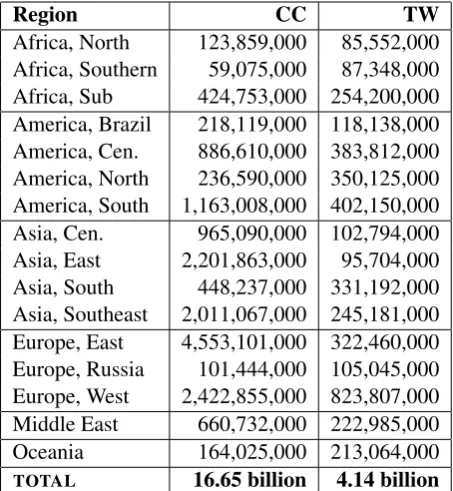
[image:2.595.307.534.62.308.2]Africa, North 123,859,000 85,552,000 Africa, Southern 59,075,000 87,348,000 Africa, Sub 424,753,000 254,200,000 America, Brazil 218,119,000 118,138,000 America, Cen. 886,610,000 383,812,000 America, North 236,590,000 350,125,000 America, South 1,163,008,000 402,150,000 Asia, Cen. 965,090,000 102,794,000 Asia, East 2,201,863,000 95,704,000 Asia, South 448,237,000 331,192,000 Asia, Southeast 2,011,067,000 245,181,000 Europe, East 4,553,101,000 322,460,000 Europe, Russia 101,444,000 105,045,000 Europe, West 2,422,855,000 823,807,000 Middle East 660,732,000 222,985,000 Oceania 164,025,000 213,064,000 TOTAL 16.65 billion 4.14 billion
Table 1: Background Corpus Size in Words by Region
important conceptual problem: when does predic-tive accuracy reflectdialectsas opposed to either place-references or place-based content? While geo-referenced corpora capture both types of in-formation, syntactic representations focus specifi-cally onlinguisticvariation while place-references and place-based topics are part of document con-tent rather than linguistic structure.
3 Where Is English Used?
The goal of this paper is to model syntactic varia-tion across all major or robust varieties of English. But how do we know which varieties should be included? Rather than select some set of varieties based on convenience, we take a data-driven ap-proach by collecting global web-crawled data and social media data to determine where English is used. This approach is biased towards developed countries with access to digital technologies. As shown in Table 1, however, enough global lan-guage data is available from both sources to de-termine where national varieties of English exist.
Data comes from two sources of digital texts: web pages from the Common Crawl1 and social media from Twitter.2 Both types of data have been used previously to study dialectal and spa-tial variation in language. More commonly, geo-referenced Twitter data has been taken to
repre-1
sent language-use in specific places (e.g., Eisen-stein, et al., 2010; Roller, et al., 2012; Kondor, et al., 2013; Mocanu, et al., 2013; Eisenstein, et al., 2014; Graham, et al., 2014; Donoso & Sanchez, 2017); regional variation in Twitter usage was also the subject of a shared task at PAN-17 (Rangel, et al., 2017). Web-crawled data has also been curated and prepared for the purpose of studying spatial variation (Goldhahn, et al., 2012; Davies & Fuchs, 2015), including the use of country-level domains for geo-referencing (Cook & Brinton, 2017). This paper builds on such previous work by system-atically collecting geo-referenced data from both sources on a global scale. The full web corpus is available for download.3
For the Common Crawl data (abbreviated as CC), language samples are geo-located using country-specific top-level domains. The assump-tion is that a language sample from a web-site un-der the.ca domain originated from Canada (c.f., Cook & Brinton, 2017). This approach to region-alization does not assume that whoever produced that language sample was born in Canada or repre-sents a traditional Canadian dialect group; rather, the assumption is only that the sample represents someone in Canada who is producing language data. Some countries are not available because their top-level domains are used for other purposes (i.e.,.ai,.fm,.io,.ly,.ag,.tv). Domains that do not contain geographic information are also removed from consideration (e.g., .com sites). The Com-mon Crawl dataset covers 2014 through the end of 2017, totalling 81.5 billion web pages. As shown in Table 1, after processing this produces a corpus of 16.65 billion words.
The basic procedure for processing the Com-mon Crawl data is to look at text within paragraph tags: any document with at least 40 words within paragraph tags from a country-level domain is pro-cessed. Noise like navigational items, boilerplate text, and error messages is removed using heuris-tic searches and also using deduplication: any text that occurs multiple times on the same site or mul-tiple times within the same month is removed. A second round of deduplication is used over the en-tire dataset to remove texts in the same language that occur in the same country. Its limited scope makes this final deduplication stage possible. For reproducibility, the code used for collecting and
3https://labbcat.canterbury.ac.nz/
download/?jonathandunn/CGLU_v3
processing the Common Crawl data is also made available.4
The use of country-level domains for geo-referencing raises two questions: First, are there many domains that are not available because they are not used or are used for non-geographic pur-poses? After removing irrelevant domains like.tv, the CC dataset covers 166 countries (30 of which are not included in the Twitter corpus) while the Twitter corpus covers 169 countries (33 of which are not included in the CC corpus). Thus, while the use of domains does remove some countries from consideration, the effect is limited. Second, does the amount of data for each country domain reflect the actual number of web pages from that country? In other words, some countries like the United States are less likely to use their top-level codes. However, the United States is still well-represented in the model. The bigger worry is that regional varieties from Africa or East Asia, both of which are under-represented in these datasets, might be missing from the model.
For the Twitter corpus, a spatial search is used to collect Tweets from within a 50km radius of 10k cities.5 Such a search avoids biasing the selection by using language-specific keywords or hashtags. The Twitter data covers the period from May of 2017 until early 2019. This creates a corpus con-taining 1,066,038,000 Tweets. The language iden-tification component, however, only provides re-liable predictions for samples containing at least 50 characters. Thus, the corpus is pruned to in-clude only those Tweets above that length thresh-old. As shown in Table 1, this produces a corpus containing 4.14 billion words with a global distri-bution. Language identification (LID) is important here because a failure to identify some regional va-rieties of English will ultimately bias the model. The LID system used is available for testing.6 But given that the focus is a major language, English, the performance of LID is not a significant factor in the overall model of syntactic variation.
The datasets summarized in Table 1 include many languages other than English. The purpose is to provide background information about where robust varieties of English are found: where is
4
https://github.com/jonathandunn/ common_crawl_corpus
5
https://github.com/datasets/ world-cities
6https://github.com/jonathandunn/
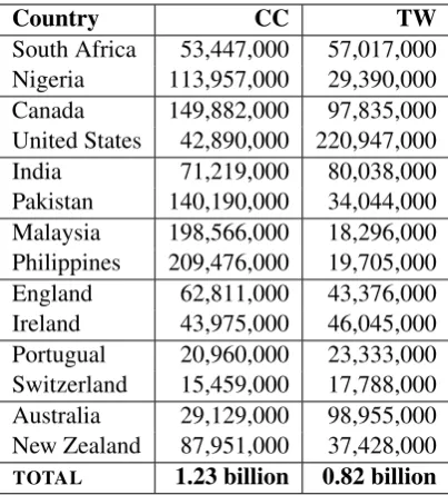
Country CC TW South Africa 53,447,000 57,017,000 Nigeria 113,957,000 29,390,000 Canada 149,882,000 97,835,000 United States 42,890,000 220,947,000 India 71,219,000 80,038,000 Pakistan 140,190,000 34,044,000 Malaysia 198,566,000 18,296,000 Philippines 209,476,000 19,705,000 England 62,811,000 43,376,000 Ireland 43,975,000 46,045,000 Portugual 20,960,000 23,333,000 Switzerland 15,459,000 17,788,000 Australia 29,129,000 98,955,000 New Zealand 87,951,000 37,428,000 TOTAL 1.23 billion 0.82 billion
Table 2: English Varieties by Dataset in N. Words
English discovered when the search is not biased by looking only for English? On the one hand, some regions may be under-represented in these datasets; if national varieties are missing from a region, it could be (i) that there is no national va-riety of English or (ii) that there is not enough data available from that region. On the other hand, Table 1 shows that each region is relatively well-represented, providing confidence that we are not missing other important varieties.
4 How Many Varieties of English?
We take a simple threshold-based approach to the question of which regional varieties to in-clude: any national variety that has at least 15 mil-lion words in both the Common Crawl and Twit-ter datasets is included in the attempt to model all global varieties of English. This threshold is chosen in order to ensure that sufficient train-ing/testing/development samples are available for each variety. The inventory of national varieties in Table 2 is entirely data-driven and does not depend on distinctions like dialects vs. varieties, inner-circle vs. outer-inner-circle, or native vs. non-native. Instead, the selection is empirical: any area with a large amount of observed English usage is as-sumed to represent a regional variety. Since the regions here are based on national boundaries, we call these national varieties. We could just as eas-ily call them national dialects.
Nevertheless, the inventory (sorted by region) contains within it some important combinations.
CC TW
[image:4.595.322.511.63.106.2]Training Samples 327,500 308,000 Testing Samples 66,500 64,000
Table 3: Samples by Function and Dataset
There are two African varieties, two south Asian varieties, two southeast Asian varieties, two native-speaker European varieties and two non-native-speaker European varieties. Taken together, these pairings provide a rich ground for exper-imentation. Are geographically closer varieties more linguistically similar? Is there an empiri-cal reality to the distinction between inner-circle and outer-circle varieties (e.g., American English vs. Malaysian English)? The importance of this language-mapping approach is that it does not as-sume the inventory of regions.
5 Data Preparation and Division
The goal of this paper is to model syntactic vari-ation using geo-referenced documents taken from web-crawled and social media corpora. Such geo-referenced documents represent language useina particular place but, unlike traditional dialect sur-veys, there is no assurance that individual authors are native speakers from that place. We have to assume that most language samples from a given country represent the native English variety of that country. For example, many non-local residents live in Australia; we only have to assume thatmost speakers observed in Australia are locals.
In order to average out the influence of out-of-place samples, we use random aggregation to cre-ate samples of exactly 1,000 words in both cor-pora. For example, in the Twitter corpus this means that an average of 59 individual Tweets from a place are combined into a single sample. First, this has the effect of providing more con-structions per sample, making the modeling task more approachable. Second and more importantly, individual out-of-place Tweets are reduced in im-portance because they are aggregated with other Tweets presumably produced by local speakers.
much larger corpora (i.e., Tweets from American English), a maximum of 25k training samples and 5k testing samples are allowed per variety per reg-ister. This creates a corpus with 327,500 train-ing and 66,500 testtrain-ing samples (CC) and a corpus with 308,000 training and 64,000 testing samples (TW). As summarized in Table 3, these datasets contain significantly more observations than have been used in previous work (c.f., Dunn, 2018c).
6 Learning the Syntactic Feature Space
Past approaches to syntactic representation for this kind of task used part-of-speech n-grams (c.f., Hirst & Feiguina, 2007) or lists of function words (c.f., Argamon & Koppel, 2013) to indirectly rep-resent grammatical patterns. Recent work (Dunn, 2018c), however, has introduced the use of a full-scale syntactic representations based on gram-mar induction (Dunn, 2017, 2018a, 2019) within the Construction Grammar paradigm (CxG: Lan-gacker, 2008; Goldberg, 2006). The idea is that this provides a replicable syntactic representation. A CxG, in particular, is useful for text classi-fication tasks because it is organized around com-plexconstructionsthat can be quantified using fre-quency. For example, the ditransitive construc-tion in (1) is represented using a sequence of slot-constraints. Some of these slots have syntactic fillers (i.e.,NOUN) and some have joint syntactic-semantic fillers (i.e., V:transfer). Any utterance, as in (2) or (3), that satisfies these slot-constraints counts as an example or instance of the construc-tion. This provides a straight-forward quantifica-tion of a grammar as a one-hot encoding of con-struction frequencies.
(1) [NOUN–V:transfer–N:animate–NOUN] (2) “He mailed Mary a letter.”
(3) “She gave me a hand.”
This paper compares two learned CxGs: first, the same grammar used in previous work (Dunn, 2018c); second, a new grammar learned with an added association-based transition extraction al-gorithm (Dunn, 2019). These are referred to as CxG-1 (the frequency-based grammar in Dunn, 2019) and CxG-2 (the association-based gram-mar), respectively. Both are learned from web-crawled corpora separate from the corpora used for modeling regional varieties (from Baroni, et al., 2009; Majli¸s & ˇZabokrtsk´y, 2012; Benko,
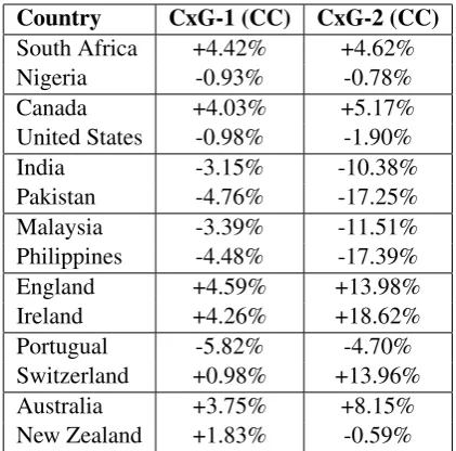
Country CxG-1 (CC) CxG-2 (CC)
South Africa +4.42% +4.62%
Nigeria -0.93% -0.78%
Canada +4.03% +5.17%
United States -0.98% -1.90%
India -3.15% -10.38%
Pakistan -4.76% -17.25%
Malaysia -3.39% -11.51%
Philippines -4.48% -17.39%
England +4.59% +13.98%
Ireland +4.26% +18.62%
Portugual -5.82% -4.70%
Switzerland +0.98% +13.96%
Australia +3.75% +8.15%
[image:5.595.311.522.61.269.2]New Zealand +1.83% -0.59%
Table 4: Relative Average Feature Density
2014; and the data provided for the CoNLL 2017 Shared Task: Ginter, et al., 2017). The exact datasets used are available.7
In both cases a large background corpus is used to represent syntactic constructions that are then quantified in samples from regional varieties. The grammar induction algorithm itself operates in folds, optimizing grammars against individual test sets and then aggregating these fold-specific grammars at the end. This creates, in effect, one large umbrella-grammar that potentially over-represents a regional dialect. From the perspec-tive of the grammar, we can think of false posiperspec-tives (the umbrella-grammar contains constructions that a regional dialect does not use) and false nega-tives (the umbrella-grammar is missing construc-tions that are important to a regional dialect). For dialect identification as a task, only missing con-structions will reduce prediction performance.
How well do CxG-1 and CxG-2 represent the corpora from each regional variety? While pre-diction accuracies are the ultimate evaluation, we can also look at the average frequency across all constructions for each national dialect. Because the samples are fixed in length, we would expect the same frequencies across all dialects. On the other hand, false positive constructions (which are contained in the umbrella-grammar but do not oc-cur frequently in a national dialect) will reduce the overall feature density for that dialect. Because the
7https://labbcat.canterbury.ac.
classification results do not directly evaluate false positive constructions, we investigate this in Ta-ble 4 using the average feature density: the total average frequency per sample, representing how many syntactic constructions from the umbrella-grammar are present in each regional dialect. This is adjusted to show differences from the average for each grammar (i.e., CxG-1 and CxG-2 are each calculated independently).
First, CxG-1 has a smaller range of feature den-sities, with the lowest variety (Portugal English) being only 10.41% different from the highest va-riety (UK English). This range is much higher for CxG-2, with a 36.01% difference between the lowest variety (Philippines English) and the high-est variety (Irish English). One potential expla-nation for the difference is that CxG-2 is a bet-ter fit for the inner-circle dominated training data. This is a question for future work. For now, both grammars pattern together in a general sense: the highest feature density is found in UK English and varieties more similar to UK English (Ireland, Australia). The lowest density is found in under-represented varieties such as Portugal English or Philippines English. Any grammar-adaptation based on dialect identification will struggle to add unknown constructions from these varieties.
7 Modeling National Varieties
The main set of experiments uses a Linear Sup-port Vector Machine (Joachims, 1998) to classify dialects using CxG features. Parameters are tuned using the development data. Given the general ro-bust performance of SVMs in the literature rela-tive to other similar classifiers on variation tasks (c.f., Dunn, et al., 2016), we forego a systematic evaluation of classifiers.
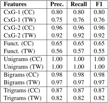
We start, in Table 5, with an evaluation of baselines by feature type and dataset. We have two general types of features: purely syntactic representations (CxG-1, CxG-2, Function words) and potentially topic-based features (unigrams, bi-grams, trigrams). The highest performing feature on both datasets is simple lexical unigrams, at 30k dimensions. We use a hashing vectorizer to avoid a region-specific bias: the vectorizer does not need to be trained or initialized against a specific dataset so there is no chance that one of the varieties will be over-represented in determining which n-grams are included. But this has the side-effect of pre-venting the inspection of individual features.
Vec-Features Prec. Recall F1
[image:6.595.321.513.62.243.2]CxG-1 (CC) 0.80 0.80 0.80 CxG-1 (TW) 0.75 0.76 0.76 CxG-2 (CC) 0.96 0.96 0.96 CxG-2 (TW) 0.92 0.92 0.92 Funct. (CC) 0.65 0.65 0.65 Funct. (TW) 0.56 0.57 0.55 Unigrams (CC) 1.00 1.00 1.00 Unigrams (TW) 1.00 1.00 1.00 Bigrams (CC) 0.98 0.98 0.98 Bigrams (TW) 0.97 0.97 0.97 Trigrams (CC) 0.87 0.87 0.87 Trigrams (TW) 0.82 0.82 0.82
Table 5: Classification Performance By Feature Set
tors for all experiments are available, along with the trained models that depend on these vectors.8
Asnincreases, n-grams tend to represent struc-tural rather than topical information. In this case, performance decreases as n increases. We sug-gest that this decrease provides an indication that the performance of unigrams is based on location-specific content (e.g., “Chicago” vs. “Singapore”) rather than on purely linguistic lexical variation (e.g., “jeans” vs. “denim”). How do we differen-tiate between predictions based on place-names, those based on place-specific content, and those based on dialectal variation? That is a question for future work. For example, is it possible to iden-tify and remove location-specific content terms? Here we focus instead on using syntactic repre-sentations that are not subject to such interference. Within syntactic features, function words per-form the worst on both datasets with F1s of 0.65 and 0.55. This is not surprising because function words in English do not represent syntactic struc-tures directly; they are instead markers of the types of structures being used. CxG-1 comes next with F1s of 0.80 and 0.76, a significant improvement over the function-word baseline but not approach-ing unigrams. Note that the experiments usapproach-ing this same grammar in previous work (Dunn, 2018c) were applied to samples of 2k words each. Fi-nally, CxG-2 performs the best, with F1s of 0.96 and 0.92, falling behind unigrams but rivaling bi-grams and surpassing tribi-grams. Because of this, the more detailed experiments below focus only on the CxG-2 grammar.
8https://labbcat.canterbury.ac.nz/
Country Prec. (CC) Recall (CC) F1 (CC) Prec. (TW) Recall (TW) F1 (TW)
South Africa 0.94 0.96 0.95 0.92 0.94 0.93
Nigeria 0.98 0.98 0.98 0.94 0.95 0.94
Canada 0.94 0.94 0.94 0.84 0.79 0.81
United States 0.93 0.95 0.94 0.85 0.89 0.87
India 0.97 0.98 0.97 0.97 0.97 0.97
Pakistan 1.00 0.99 0.99 0.98 0.98 0.98
Malaysia 0.96 0.96 0.96 0.99 0.99 0.99
Philippines 0.98 0.97 0.98 0.98 0.98 0.98
England 0.95 0.95 0.95 0.87 0.90 0.89
Ireland 0.97 0.97 0.97 0.95 0.95 0.95
Portugual 0.99 0.98 0.98 0.93 0.90 0.92
Switzerland 0.97 0.94 0.96 0.98 0.97 0.97
Australia 0.97 0.96 0.97 0.82 0.83 0.83
New Zealand 0.91 0.92 0.91 0.92 0.90 0.91
[image:7.595.81.521.60.285.2]W. AVG 0.96 0.96 0.96 0.92 0.92 0.92
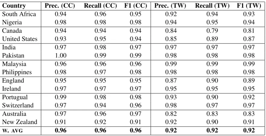
Table 6: Within-Domain Classification Performance (CxG-2)
A closer look at both datasets by region for CxG-2 is given in Table 6. The two datasets (web-crawled and social media) present some interest-ing divergences. For example, Australian English is among the better performing varieties on the CC dataset (F1 = 0.97) but among the worst per-forming varieties on Twitter (F1 = 0.83). This is the case even though the variety we would assume would be most-often confused with Australian En-glish (New Zealand EnEn-glish) has a stable F1 across domains (both are 0.91). An examination of the confusion matrix (not shown), reveals that errors between New Zealand and Australia are similar between datasets but that the performance of Aus-tralian English on Twitter data is reduced by con-fusion between Australian and Canadian English.
In Table 4 we saw that the umbrella-grammar (here, CxG-2) better represents inner-circle vari-eties, specifically UK English and more closely related varieties. This is probably an indication of the relative representation of the different vari-eties used to train the umbrella-grammar: gram-mar induction will implicitly model the variety it is exposed to. It is interesting, then, that less typi-cal varieties like Pakistan English and Philippines English (which had lower feature densities) have higher F1s in the dialect identification task. On the one hand, the syntactic differences between these varieties and inner-circle varieties means that the umbrella-grammar misses some of their unique constructions. On the other hand, their greater syntactic difference makes these varieties easier to
identify: they are more distinct in syntactic terms even though they are less well represented.
Which varieties are the most similar syntacti-cally given this model? One way to quantify simi-larity is using errors: which varieties are the most frequently confused? American and Canadian En-glish have 221 misclassified samples (CC), while Canadian and UK English are only confused 36 times. This reflects an intuition that Canadian En-glish is much more similar to American EnEn-glish than it is to UK English. New Zealand and Aus-tralian English have 101 misclassifications (again, on CC); but New Zealand and South African En-glish have 266. This indicates that New Zealand English is more syntactically similar to South African English than to Australian English. How-ever, more work on dialect similarity is needed to confirm these findings across different datasets.
8 Varieties on the Web and Social Media
Country Prec. (CC) Recall (CC) F1 (CC) Prec. (TW) Recall (TW) F1 (TW)
South Africa 0.88 0.06 0.10 0.68 0.31 0.43
Nigeria 0.43 0.84 0.57 0.73 0.41 0.52
Canada 0.48 0.14 0.22 0.49 0.27 0.35
United States 0.20 0.87 0.32 0.83 0.16 0.27
India 0.65 0.94 0.77 0.38 0.90 0.54
Pakistan 0.96 0.41 0.58 0.88 0.36 0.51
Malaysia 0.45 0.93 0.61 0.98 0.05 0.10
Philippines 0.73 0.61 0.66 0.87 0.22 0.35
England 0.89 0.01 0.03 0.48 0.44 0.46
Ireland 0.94 0.21 0.35 0.78 0.52 0.62
Portugual 0.02 0.00 0.00 0.22 0.17 0.19
Switzerland 0.92 0.04 0.07 0.12 0.80 0.20
Australia 0.89 0.00 0.00 0.33 0.66 0.44
New Zealand 0.27 0.53 0.36 0.64 0.40 0.49
[image:8.595.83.517.60.286.2]W. AVG 0.62 0.40 0.33 0.62 0.40 0.40
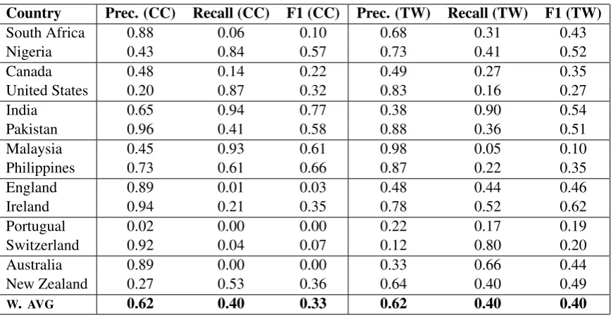
Table 7: Cross-Domain Models, Trained on CC (Left) and Trained on TW (Right), CxG-2
Country Prec. Recall F1
South Africa 0.91 0.92 0.92
Nigeria 0.94 0.95 0.95
Canada 0.87 0.84 0.85
United States 0.85 0.90 0.87
India 0.96 0.97 0.97
Pakistan 0.98 0.98 0.98 Malaysia 0.97 0.96 0.96 Philippines 0.97 0.97 0.97
England 0.87 0.90 0.89
Ireland 0.94 0.95 0.95
[image:8.595.91.272.323.545.2]Portugual 0.94 0.90 0.92 Switzerland 0.96 0.93 0.95 Australia 0.87 0.86 0.87 New Zealand 0.89 0.87 0.88 W. AVG 0.92 0.92 0.92
Table 8: Single-Set Classification Performance
does Australian English have the same profile on both the web and on Twitter?
Starting with the register-agnostic experiments, Table 8 shows the classification performance if we lump all the samples into a single dataset (how-ever, the same training and testing data division is still maintained). The overall F1 is the same as the Twitter-only results in Table 6. On the other hand, varieties like Australian English that per-formed poorly in Twitter perform somewhat better under these conditions. Furthermore, the obser-vation made above that outer-circle varieties are more distinct remains true: the highest
perform-ing varieties are the least proto-typical (i.e., Indian English and Philippines English).
But a single model does not perform well across the two datasets, as shown in Table 7. The model trained on Twitter data does perform somewhat better than its counterpart, but in both cases there is a significant drop in performance. On the one hand, this is not surprising given differences in the two registers: we expect some reduction in classi-fication performance across domains like this. For example, the unigram baseline suffers a similar re-duction to F1s of 0.49 (trained on CC) and 0.55 (trained on Twitter).
On the other hand, we would have more confi-dence in this model of syntactic variation if there was a smaller drop in accuracy. How can we bet-ter estimate grammars and variations in grammars across these different registers? Is it a problem of sampling different populations or is there a single population that is showing different linguistic be-haviours? These are questions for future work.
9 Unmasking Dialects
0.75 0.8 0.85 0.9 0.95 1 1.05
1 5 9 13 17 21 25 29 33 37 41 45 49 53 57 61 65 69 73 77 81 85 89 93 97
[image:9.595.79.508.67.255.2]CxG-2 (CC) Unigrams (CC) CxG-2 (TW) Unigrams (TW)
Figure 1: Performance Over 100 Rounds of Unmasking (F1)
the texts as samples. Here we distinguish between dialects with individual samples as chunks. After each round of classification, the most predictive features are removed. In this case, the highest pos-itive and negative features for each regional dialect are removed for the next classification round. Fig-ure 1 shows the unmasking curve over 100 rounds using the F1 score. Given that there are 14 re-gional dialects in the model, Figure 1 represents the removal of approximately 2,800 features.
For both datasets, the unigram baseline de-grades less quickly than the syntactic model. On the one hand, it has significantly more features in total, so that there are more features to support the classification. On the other hand, given that the most predictive features are being removed, this shows that the lexical model has a deeper range of differences available to support classification than the syntactic model. Within the syntactic mod-els, the classifier trained on web-crawled data de-grades less quickly than the Twitter model and maintains a higher performance throughout.
This unmasking curve is simply a method for vi-sualizing the robustness of a classification model. The syntactic model is less robust to unmasking than the lexical model. At the same time, we know that the syntactic model does not rely on place-names and place-based content and thus represents a more traditional linguistic approach to variation.
10 Discussion
This paper has used data-driven language mapping to select national dialects of English to be included
in a global dialect identification model. The main experiments have focused on a dynamic syntac-tic feature set, showing that it is possible to pre-dict dialect membership within-domain with only a small loss of performance against lexical mod-els. This work raises two remaining problems:
First, we know that location-specific content (i.e., place names, place references, national events) can be used for geo-location and text-based models of place. To what degree does a lexical approach capture linguistic variation (i.e., “pop” vs. “soda”) and to what degree is it captur-ing non-lcaptur-inguistic information (i.e., “Melbourne” vs. “London”)? This is an essential problem for dialect identification models. A purely syntactic model does not perform as well as a lexical model, but it does come with more guarantees.
References
Adams, B. 2015. Finding Similar Places using the Observation-to-Generalization Place Model. Jour-nal of Geographical Systems, 17(2): 137-156.
Adams, B. and McKenzie, G. 2018. Crowdsourc-ing the character of a place: Character-level con-volutional networks for multilingual geographic text classification. Transactions in GIS, doi: 10.1111/tgis.12317.
Ali, M. 2018. Character Level Convolutional Neural Network for Arabic Dialect Identification. In Pro-ceedings of the Fifth Workshop on NLP for Similar Languages, Varieties and Dialects, 122-127.
Argamon, S. and Koppel, M. 2013. A Systemic Func-tional Approach to Automated Authorship Analysis.
Journal of Law & Policy, 12:299-315.
Barbaresi, A. 2018. Computationally efficient discrim-ination between language varieties with large fea-ture vectors and regularized classifiers. In Proceed-ings of the Fifth Workshop on NLP for Similar Lan-guages, Varieties and Dialects, 164-171.
Baroni, M., Bernardini, S., Ferraresi, A., and Zanchetta, E. 2009. The WaCky Wide Web: A Col-lection of Very Large Linguistically Processed Web-crawled Corpora. Language Resources and Evalua-tion, 43: 209-226.
Belinkov, Y. and Glass, J. 2016. A Character-level Convolutional Neural Network for Distinguishing Similar Languages and Dialects. InProceedings of the Third Workshop on NLP for Similar Languages, Varieties and Dialects, 145-152.
Benko, V. 2014. Aranea: Yet Another Family of (Comparable) Web Corpora. InProceedings of Text, Speech and Dialogue. 17th International Confer-ence. 257-264.
Calle-Martin, J. and Romero-Barranco, J. 2017. Third person present tense markers in some varieties of English. English World-Wide, 38(1): 77-103.
Clark, L and Watson, K. 2016. Phonological leveling, diffusion, and divergence: /t/ lenition in Liverpool and its hinterland. Language Variation and Change, 28(1): 31-62.
Collins, P. 2012. Singular agreement in there-existentials: An intervarietal corpus-based study.
English World-Wide, 33(1): 53-68.
Cook, P. and Brinton, J. 2017. Building and evaluating web corpora representing national varieties of En-glish. Language Resources and Evaluation, 51.
Davies, M. and Fuchs, R. 2015. Expanding horizons in the study of World Englishes with the 1.9 billion word Global Web-based English Corpus (GloWbE).
English World-Wide, 36(1): 1-28.
Donoso, G. and Sanchez, D. 2017. Dialectometric analysis of language variation in twitter. In Pro-ceedings of the 4th Workshop on NLP for Similar Languages, Varieties and Dialects. 16-25.
Dunn, J. 2017. Computational Learning of Construc-tion Grammars. Language & Cognition, 9(2): 254-292.
Dunn, J. 2018a. Modeling the Complexity and De-scriptive Adequacy of Construction Grammars. In
Proceedings of the Society for Computation in Lin-guistics (SCiL 2018). Stroudsburg, PA: Association for Computational Linguistics. 81-90.
Dunn, J. 2018b. Multi-Unit Directional Measures of Association: Moving Beyond Pairs of Words. Inter-national Journal of Corpus Linguistics, 23(2): 183-215.
Dunn, J. 2018c. Finding Variants for Construction-Based Dialectometry: A Corpus-Construction-Based Approach to Regional CxGs. Cognitive Linguistics, 29(2): 275-311.
Dunn, J. 2019. Frequency vs. Association for Constraint Selection in Usage-Based Construction Grammar. InProceedings of the Workshop on Cog-nitive Modeling and Computational Linguistics. As-sociation for Computational Linguistics.
Dunn, J.; Argamon, S.; Rasooli, A.; and Kumar, G. 2016. Profile-based authorship analysis. Literary and Linguistic Computing, 31(4): 689-710.
Eisenstein, J.; O’Connor, B.; Smith, N.; and Xing, E. 2010. A latent variable model for geographic lexi-cal variation. InProceedings of the Conference on Empirical Methods in Natural Language Process-ing, 1,227-1,287.
Eisenstein, J.; O’Connor, B.; Smith, N.; and Xing, E. 2014. Diffusion of lexical change in social media.
PloSOne, 10.1371.
Gamallo, P.; Pichel, J.; Algeria, I.; and Agirrezabal, M. 2016. Comparing two Basic Methods for Discrimi-nating Between Similar Languages and Varieties. In
Proceedings of the Third Workshop on NLP for Sim-ilar Languages, Varieties and Dialects, 170-177.
Ginter, F.; Hajiˆc, J.; Luotolahti, J. 2017. CoNLL 2017 Shared Task - Automatically Annotated Raw Texts and Word Embeddings, LIN-DAT/CLARIN digital library at the Institute of Formal and Applied Linguistics ( ˜AˇsFAL), Faculty of Mathematics and Physics, Charles University. http://hdl.handle.net/11234/1-1989.
Goldberg, A. 2006. Constructions at Work: The Na-ture of Generalization in Language. Oxford: Ox-ford University Press.
Leipzig Corpora Collection: From 100 to 200 Lan-guages. InProceedings of the Conference on Lan-guage Resources and Evaluation.
Grafmiller, J. & Szmrecsanyi, B. 2018. Mapping out particle placement in Englishes around the world: A study in comparative sociolinguistic analysis. Lan-guage Variation and Change, 30(3): 385-412.
Graham, S.; Hale, S.; and Gaffney, D. 2014. Where in the world are you? Geolocation and language iden-tification on twitter. The Professional Geographer, 66(4).
Grieve, J. 2007. Quantitative Authorship attribution: an evaluation of techniques. Literary and Linguistic Computing, 22(3): 251–70.
Hirst, G. and Feiguina, O. 2007. Bigrams of syntactic labels for authorship discrimination of short texts.
Literary and Linguistic Computing, 22(4): 405–17.
Hulden, M.; Silfverberg, M.; and Francom, J. 2015. Kernel Density Estimation for Text-Based Geoloca-tion. InProceedings of the Twenty-Ninth AAAI Con-ference on Artificial Intelligence, 145-150.
Ionescu, R. and Popescu, M. 2016. UnibucKernel: An Approach for Arabic Dialect Identification based on Multiple String Kernels. InProceedings of the Third Workshop on NLP for Similar Languages, Varieties and Dialects, 135-144.
Joachims, T. 1998. Text categorization with support vector machines: Learning with many relevant fea-tures. In C. Nedellec (ed.), Machine learning: ECML-98: 10th European Conference on Machine Learning, 137-142. Berlin: Springer.
Ju, Y.; Adams, B.; Janowicz, K.; Hu, Y.; Yan, B.; and McKenzie, G. 2016. Things and Strings: Improv-ing Place Name Disambiguation from Short Texts by Combining Entity Co-Occurrence with Topic Mod-eling. InProceedings of the 20th International Con-ference on Knowledge Engineering and Knowledge Management. LNCS, vol. 10024. Springer, pp. 353-367.
Kachru, B. 1990 The Alchemy of English: The spread, functions, and models of non-native En-glishes. Urbana-Champaign: University of Illinois Press.
Kondor, D.; Csabai, I.; Dobos, L.; Szule, J.; Barankai, N.; Hanyecz, T.; Sebok, T.; Kallus, Z.; and Vattay, G. 2013. Using robust PCA to estimate regional characteristics of language-use from geotagged twit-ter messages. In Proceedings of IEEE 4th Interna-tional Conference on Cognitive Infocommunications (CogInfoCom). 393-398.
Koppel, M., J. Schler, and E. Bonchek-Dokow. 2007. Measuring Differentiability: Unmasking Pseudony-mous Authors. Journal of Machine Learning Re-search, 8: 1261-1276.
Kreutz, T. and Daelemans, W. 2018. Exploring Clas-sifier Combinations for Language Variety Identifica-tion. InProceedings of the Fifth Workshop on NLP for Similar Languages, Varieties and Dialects, 191-198.
Kroon, M.; Medvedeva, M.; and Plank, B. 2018. When Simple n-gram Models Outperform Syntactic Ap-proaches: Discriminating between Dutch and Flem-ish. InProceedings of the Fifth Workshop on NLP for Similar Languages, Varieties and Dialects, 244-25.
Kruger, H. and van Rooy, Bertus. 2018. Register vari-ation in written contact varieties of English: A mul-tidimensional analysis. English World-Wide, 39(2): 214-242.
Labov, W.; Fisher, S.; Gylfadottir, D.; and Hender-son, A. 2016. Competing systems in Philadelphia phonology.Language Variation and Change, 28(3): 273-305.
Langacker, R. 2008. Cognitive Grammar: A Basic In-troduction. Oxford: Oxford University Press.
Lourentzou, I.; Morales, A.; and Zhai, C. 2017. Text-based geolocation prediction of social media users with neural networks. InProceedings of 2017 IEEE International Conference on Big Data, 696-705.
McNamee, P. 2016. Language and Dialect Discrimina-tion Using Compression-Inspired Language Models. In Proceedings of the Third Workshop on NLP for Similar Languages, Varieties and Dialects, 195-203.
Mocanu, D.; Baronchelli, A.; Perra, N.; Gon ˜A§alves, B.; Zhang, Q. and Vespignani, A. 2013. The Twit-ter of Babel: Mapping world languages through mi-croblogging platforms. PLOSOne, 10.1371.
Majli¸s, M. and Z¸ abokrtsk´y, Z. 2012. Language Rich-ness of the Web. InProceedings of the International Conference on Language Resources and Evaluation (LREC 2012). https://ufal.mff.cuni.cz/w2c.
Rangel F., Rosso P., Potthast M., Stein B. 2017. Overview of the 5th Author Profiling Task at PAN 2017: Gender and Language Variety Identification in Twitter. In: Cappellato L., Ferro N., Goeu-riot L, Mandl T. (eds.)CLEF 2017 Labs and Work-shops, Notebook Papers. CEUR Workshop Proceed-ings.CEUR-WS.org, vol. 1866.
Roller, S.; Speriosu, M.; Rallapalli, S.; Wing, B.; and Baldridge, J. 2012. Supervised text-based geoloca-tion using language models on an adaptive grid. In
Proceedings of the 2012 Joint Conference on Empir-ical Methods in Natural Language Processing and Computational Natural Language Learning. 1,500-1,510.
Sanders, N. 2010. A statistical method for syntactic di-alectometry. Bloomington: Indiana. University dis-sertation.
Schilk, M. and Schaub, S. 2016. Noun phrase com-plexity across varieties of English: Focus on syn-tactic function and text type. English World-Wide, 37(1): 58-85.
Schreier, D. 2016. Super-leveling, fraying-out, inter-nal restructuring: A century of present be concord in Tristan da Cunha English. Language Variation and Change, 28(2): 203-224.
Strelluf, C. 2016. Overlap among back vowels before /l/ in Kansas City. Language Variation and Change, 28(3): 379-407.
Szmrecsanyi, B.; Grafmiller, J.; Heller, B.; Rothlis-berger, M. 2016. Around the world in three alter-nations: Modeling syntactic variation in varieties of English. English World-Wide, 37(2): 109-137.
Tamaredo, I. 2018. Pronoun omission in high-contact varieties of English: Complexity versus efficiency.
English World-Wide, 39(1): 85-110.
Wing, B. and Baldridge, J. 2014. Hierarchical Dis-criminative Classification for Text-Based Geoloca-tion. InProceedings of the Conference on Empirical Methods in NLP, 336-348.
Zeman, D., et al. 2017. CoNLL 2017 Shared Task: Multilingual Parsing from Raw Text to Universal Dependencies. InProceedings of the Conference on Natural Language Learning, 1-19.