Model driven engineering of planning and optimisation algorithms for pervasive computing environments

(1)

Model-Driven Engineering of Planning and

Optimisation Algorithms for Pervasive Computing

Environments

Anthony Harrington

1

and Vinny Cahill

1,2

Distributed Systems Group1

Lero - The Irish Software Engineering Centre2

School of Computer Science and Statistics Trinity College Dublin

Email: [email protected]

Abstract—This paper presents a model-driven approach to developing pervasive computing applications that exploits design-time information to support the engineering of planning and optimisation algorithms that reflect the presence of uncertainty, dynamism and complexity in the application domain. In par-ticular the task of generating code to implement planning and optimisation algorithms in pervasive computing domains is addressed.

We present a layered domain model containing a set of object-oriented specifications for modelling physical and sensor/actuator infrastructure and state-space information. Our model-driven engineering approach is implemented in two transformation algo-rithms. The initial transformation parses the domain model and generates a planning model for the application being developed that encodes an application’s states, actions and rewards. The second transformation parses the planning model and selects and seeds a planning or optimisation algorithm for use in the application.

We present an empirical evaluation of the impact of our approach on the development effort associated with a pervasive computing application from the Intelligent Transportation Sys-tems (ITS) domain, and provide a quantitative evaluation of the performance of the algorithms generated by the transformations.

I. INTRODUCTION

This paper addresses the challenges involved in engineering pervasive computing applications that make use of planning and optimisation algorithms. We define a pervasive computing environment as a region of the physical environment that is augmented with sensor and actuator devices, and pervasive computing applications as those that execute in such an aug-mented physical space. Canonical examples of such applica-tions are the control of transportation infrastructures, activities such as region-wide pollution monitoring, and emergency-service management.

The complexity of real-world domains, the inference of sys-tem state from noisy sensor data, and the possible unreliability of actuator platforms used for action execution motivates the use of stochastic planning algorithms [1] in pervasive com-puting applications. Although the formal foundations of large-scale planning and acting algorithms are well established, the practical task of applying these formal foundations to large-scale problems remains challenging [2]. Furthermore

knowl-edge of such algorithms is not widespread among software development practitioners being more typically confined to the research community.

Our work focuses on those pervasive computing applications that use sensor data to infer values for application states in order to plan and take action in accordance with user-specified objectives or to optimise application states. An example would be to optimise traffic light settings in an urban traffic control (UTC) system to minimise waiting time for vehicles.

In this paper we first present a layered domain model that provides a set of object-oriented specifications for modelling physical and sensor/actuator infrastructure and application state spaces in pervasive computing environments. These spec-ifications are implemented using the XML and SQL standards. All domain-model elements are tagged with a spatial context and are combined using spatial queries to support state infer-ence routines.

We then present two transformation algorithms that parse domain models to generate application code providing plan-ning and optimisation functionality. The initial transformation algorithm parses a domain model and populates a planning model whose components provide an API for accessing appli-cation states, actions, and rewards.

The second transformation algorithm uses planning model components and generates control units for an application. A control unit is a piece of executable code implementing the planning or optimisation algorithms used in the decision/exe-cution cycle of an application. Planning model components provide an API, invoked by control units at runtime, that exposes application states as likelihood values given the spread and quality of sensor infrastructure in the environment.

The broad range of potential applications precludes a uni-fied algorithmic approach to the solution of such problems. Our approach supports an extensible library of planning and optimisation algorithms. Application developers can specify an algorithm to be used or they can allow the transformations to automatically select an appropriate, although not necessarily optimal, algorithm for the application. We provide a library of algorithms and the automated transformations seed

(2)

tions of these algorithms with data from the planning model. The criteria used to select appropriate algorithms are derived from encoding existing best practice from the literature.

Our work synthesises concepts from the fields of model driven engineering (MDE) and automated planning. Auto-mated planning focuses on the design and use of information processing tools that give access to affordable and efficient planning resources [2]. Automated planners take as input a description of the problem to be solved and produce as output a plan to govern the actions taken by an application. Because we wish to support a wide variety of problem types, we also provide support for optimisation algorithms.

The MDE component of our work addresses software engi-neering challenges associated with developing the target class of pervasive computing applications by raising the level of abstraction at which applications are developed and providing automated generation of code. The automated planning com-ponent allows specialist knowledge to be encoded in the tool-chain and reduces the knowledge of planning and optimisation algorithms required by developers. We believe that the MDE and automated planning components combine to provide a novel programming model that simplifies the provision of planning and optimisation functionality in pervasive comput-ing applications.

The remainder of this paper is structured as follows. In section II we present the development process supported by our approach. In section III we summarise the design of our domain model, an earlier version of which, has been presented in [3]. In Section IV we present the transformation algorithms used to generate application control units. Finally, we evaluate the impact of the programming model on algorithm devel-opment effort and describe the performance of a generated algorithm for a representative application scenario.

II. DEVELOPMENTPROCESS

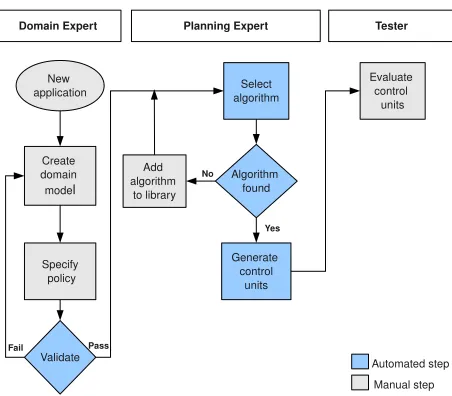
The development process accommodates two development

roles and one testing role. A domain expert defines the

application state space and specifies the application policy. Domain experts are not required to be proficient in the field

of planning and optimisation. A planning expert adds new

planning and optimisation algorithms to the library and defines mappings from our planning model API to algorithm logic. The planning expert can add algorithms without reference to pervasive computing middleware services or sensor and

actuator placement. Atester evaluates the performance of the

generated code.

Fig. 1 shows a data flow diagram for the development process. The following tool support is provided:

• A suite of domain model XML schemas.

• A validation engine to check the validity of domain

models.

• A transformation engine to parse a domain model and

populate a planning model that provides an API for use by planning and optimisation algorithms.

• A transformation engine to choose a suitable algorithm

and generate application code.

Create domain model

Validate

Domain Expert Planning Expert Tester

New application

Specify policy

Select algorithm

Algorithm found

Generate control

units Add

algorithm to library

Pass Fail

Yes No

Evaluate control

units

[image:2.612.325.551.49.247.2]

Automated step Manual step

Fig. 1. Development process roles and tool support.

• A library of planning and optimisation algorithms.

• An evaluation platform to test the performance of

gener-ated application code. This platform provides simulgener-ated sensor data and run-time middleware services for sensor and actuator discovery and access.

The tool chain is used as follows:

1) Construct a domain model using the XML schemas provided.

2) Write a policy file specifying the desired behaviour of the application.

3) The first transformation supports the validation of the domain model and policy and the generation of a plan-ning model for the application.

4) The second transformation supports the validation of the planning model and the taxonomy linking problem to algorithm type. It can also select an algorithm type to use and can generate the control units for an application. The planning expert adds new planning and optimisation algorithm implementations to the library and updates the algorithm taxonomy to specify the problem type and set of environmental conditions in which the algorithm is suitable for use. When an algorithm is added to the taxonomy a function is defined by the planning expert to map algorithm logic onto planning model components. This is a one-time effort and once the mapping has been specified, the algorithm can be repeatedly applied to new matching problem instances. The mapping logic varies with the algorithm type. Planning model components provide an API to planning experts that abstracts away from sensor and actuator placement and quality to expose run-time application state values as discrete and continuous likelihood functions. Planning model components also provide access to reward model and state-transition infor-mation, defined by the domain expert using the domain-model specifications.

(3)

the control units make use of a middleware for access and query operations. The control units operate by providing information for sensor/actuator selection and identification and assume middleware abstractions for discovery and lookup ser-vices. Such abstractions are provided by a range of pervasive computing middlewares such as [4] [5] and are not directly addressed in this paper.

III. DOMAINMODEL ANDPOLICYSPECIFICATION

The domain model contains abstractions for specifying the sensors and actuators present and the state space of a pervasive computing application. The domain model uses a topographical approach to model the spatial relationships of sensors, actuators, policies, and states as geometric shapes defined by sequences of coordinates based on a chosen, well-known coordinate system.

The domain model specifications are organised in four logical layers. Layer 1 holds static data about application relevant artefacts in the environment that is known at design-time. Layer 2 holds meta-data on the sensors and actuators in the environment that are used at runtime when determining and modifying application state. Layer 3 describes the application state space and layer 4 holds domain-specific knowledge that can be used to select and customise planning and optimisation algorithms.

To help clarify the presentation of the domain model and transformations, we first introduce a scenario in which our development process is applied to developing an application to optimise the use of CCTV camera infrastructure in a city.

A. Scenario

We assume that the city contains hundreds of CCTV sensors placed at various traffic junctions and that at any one time there may be up to 10 council staff on duty to monitor and detect traffic accidents and congestion using 30 screens that can be used to display CCTV image streams. The desired behaviour is

to select the 30 mostinterestingCCTV data streams to display

from the hundreds of available cameras. The criteria by which a CCTV camera is considered interesting, are defined by the domain expert to be a function of weather, traffic demand and pedestrian presence. There is a further requirement that the set of useful CCTV cameras should be chosen to also provide the maximal geographic spread or coverage over the city transport network.

This application therefore requires a bi-criteria optimisation algorithm to be deployed in a pervasive computing environ-ment and the use of inference techniques to infer application states from sensor data.

B. Domain Model Specifications

Layer 1 is used to specify infrastructural elements that exist in the deployment environment. Infrastructural elements characterise physical artefacts relevant to the application being developed. All layer 1 elements have a spatial attribute.

Layer 1 of the scenario domain model specifies the city’s static road network infrastructure specified as a series of

Model Element

type : int dataSourceID : int

Actuator Element

name : String mobile : boolean Sensor Element

name : String mobile : boolean

Location Reference

referenceSystemID : int location : String

Data

name : String cost : int confidence : float

Action

id : String cost : int confidence : float transition : String 1

1..* 1

0..1

1 1 1

[image:3.612.368.514.53.228.2]

1

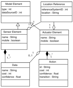
Fig. 2. Domain model sensor and actuator layer.

signalised junctions connected by road links that allow traffic to flow from one junction to another. A standard model is used to represent the road network based on the Paramics

traffic simulator1_{. This data is formatted using the SFS spatial}

data standard and stored in a PostgreSQL GIS database. There are 247 junction elements whose spatial attributes are represented as circles of radius 20 metres from junction centre points and 2800 road link elements whose spatial attributes are represented as multi-polygon geometries summing the geometries of road links. Layer 1 data was obtained from a Paramics model of Dublin city.

Layer 2 specifications are used to model the sensor and actuator infrastructure in the deployment environment. Layer 2 holds meta-data describing the data produced by the sensor and actuator infrastructure. All layer 2 elements have a spatial attribute. The spatial attribute of a sensor includes both its physical location and sensing range. Layer 2 data is used to build queries to middleware services for accessing sensors and actuators at runtime. The domain model does not hold sensor data readings or information on actions being executed by actuator infrastructure. Sensor data will be accessed at runtime through a pervasive computing middleware service.

The design of this layer is shown in Fig. 2. Sensor and Actuator classes inherit from a base Model Element class and both have an associated spatial attribute. Layer 2 sensor objects contain one or more data objects used to specify what values the sensor provides, and an actuator object contains zero or more data objects and one or more action objects used to spec-ify what actions an actuator supports. Data and action objects are used at runtime when interpreting sensor and actuator data. Data objects have a confidence attribute indicating the degree of confidence associated with individual sensor readings. For discrete sensor data the confidence measure is a probability value between 0 and 1 indicating the likelihood of sensor data being correct. For continuous sensor data the confidence value is the variance associated with sensor readings. Determining

(4)

the confidence value for a particular sensor will require either the use of self-describing sensors [6], or else may be obtained from sensor specifications and manufacturer documentation.

Actuators implement actions that may effect a change in the state of a system. The spatial attribute of an actuator includes its location and the region of the environment over which its actions have an effect. Action objects have a confidence attribute which is a probability assigned to a successful state transition caused by the actuator.

The effects of actions are specified using state charts. The domain model implementation uses a modified version of the State Chart XML (SCXML) language, which specifies state transition information based on Harel State Tables and which supports composite state spaces and probabilistic transitions [7], thus making it suitable for specifying state charts for pervasive computing environments.

Layer 2 of the scenario domain model contains three sensor elements and one actuator element. An Inductive Loop sensor [8] provides sensor data on traffic demand and travel times. Weather station sensors are modelled to provide data on rain fall levels at each junction. We also assume that a stationary pedestrian presence sensor is present at each junction to provide data on pedestrian levels. The spatial attribute of the weather and pedestrian sensors is specified as an ellipse representing their sensing areas.

Layer 3 is used to specify the state-space of a pervasive computing application. Determining state values typically re-quires access to sensors and actuators distributed throughout the environment, the quality and spread of which will often be unknown at design time. Layer 3 system-state elements are used by domain experts to specify the logic for calculating the values of application states, independently of run-time conditions. System-state elements are composed using layer 1 and 2 elements to specify the types of sensor data and actuator actions, and the types of infrastructure in the deployment environment, that are required to calculate run-time values for the application state space.

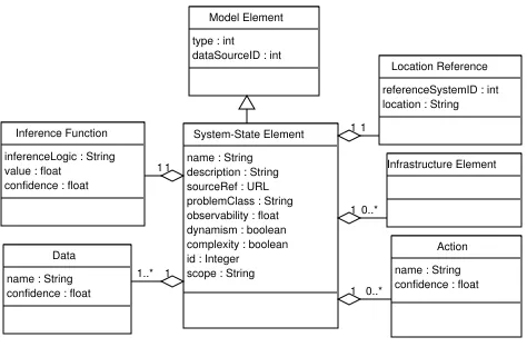
Examples of system-states include vehicle throughput at a traffic junction, journey time along a road link and power consumption in a room. The design of this layer is shown in Fig. 3. Each system-state has a scope that indicates the region of the deployment environment over which it is defined. Layer 1 and 2 elements referenced in a system-state definition are mapped at runtime onto physical entities in the region of the deployment environment described by the scope.

A system-state specification includes an inference function whose logic is used to calculate state values from the run-time values of sensor data and actuator actions. Sensor and actuator meta-data are used in the inference function to quantify the uncertainty associated with state values. Uncertainty is specified using discrete and continuous likelihood functions for the true value of the system-state given the available sensor data.

System-state elements have a problemClass attribute in-dicating that the element belongs to either a planning or optimisation problem. Deployment environment conditions

Model Element

type : int dataSourceID : int

System-State Element

name : String description : String sourceRef : URL problemClass : String observability : float dynamism : boolean complexity : boolean id : Integer scope : String Data

name : String confidence : float

Action

name : String confidence : float Infrastructure Element

Location Reference

referenceSystemID : int location : String

1 1..*

1 0..* 1 0..* 1 1 Inference Function

inferenceLogic : String value : float confidence : float

[image:4.612.320.557.53.209.2]

1 1

Fig. 3. Domain model system-states layer.

are specified using dynamism, complexity, and observability attributes that are used to indicate respectively: that the state’s value can be affected by uncontrolled state-transition events; that it may be computationally difficult to compute the value of a system-state; and that the application state space values are expressed as probabilities rather than direct observations. In the event that the domain expert does not specify which planning or optimisation algorithm to use, the transformations will use these four attributes to select an appropriate planning or optimisation algorithm for the problem.

Layer 3 of the scenario domain model contains specifi-cations of three system-states: JunctionInterest, MaximalDis-tance, and DegreeofInterest. A JunctionInterest system-state is specified to be a monotonically increasing function of wors-ening weather conditions, pedestrian presence, and increasing traffic demand. Domain experts specify system-states in XML and the XML specification of the JunctionInterest system-state is shown in Listing 1. The dynamism and observability attributes are specified to be “true” and “partial” respectively, and the complexity attribute is set to “false”. The scope of the system-state is defined as being of type “element” and of value “junction”, meaning that a value for this system-state is to be calculated at each instance of a junction infrastructure element contained in the scenario domain model. The implementation attribute contains a reference to an inference function that uses a Bayesian network to combine the inputs to produce an output value for the system-state.

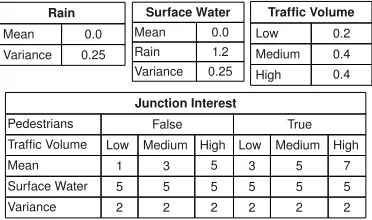
Fig. 4 shows the conditional probability tables specified in the inference function. The hybrid Bayesian network con-tains a discrete Boolean Pedestrian node indicating whether pedestrians are present or not and a discrete TrafficVolume node taking the values: “high”; “medium” and “low”. It also contains continuous SurfaceWater, Rain and JunctionInterest nodes. A sample conditional probability from Fig. 4 reads

P(Surf aceW ater|Rain) = N(1.2×Rain,0.25), i.e., the continuous variable SurfaceWater has a mean value that is

20% higher than the values reported by the Rain sensor and

a constant variance of0.25. Such a specification might reflect

(5)

<s y s t e m S t a t e> 001

<!₋₋ I m p l e m e n t a t i o n s ₋₋>

</ s y s t e m S t a t e>

Listing 1. JunctionInterest system-state definition.

Rain

Mean 0.0 Variance 0.25

Traffic Volume

Low 0.2 Medium 0.4 High 0.4

Junction Interest

Pedestrians False True Traffic Volume Low Medium High Low Medium High Mean 1 3 5 3 5 7 Surface Water 5 5 5 5 5 5 Variance 2 2 2 2 2 2

Surface Water

[image:5.612.82.268.340.450.2]

Mean 0.0 Rain 1.2 Variance 0.25

Fig. 4. Bayesian network conditional probabilities from JunctionInterest inference function.

underestimate the amount of surface water by20%.

The MaximalDistance system-state is defined to measure the geographic spread of the candidate set of CCTV cameras. To measure the geographic spread, sets of 30 selected cameras are modelled as nodes in a fully connected network. The length of all network edges (distance between junctions) is measured in metres to obtain the total length of the network and used as a measure of coverage. This state is specified to be complex, static and fully observable as the complexity of an exhaustive

search of this space isO(cn₎

wherenis the number of nodes

andc >1.

The DegreeofInterest system-state is defined to sum the JunctionInterest value for each junction in the candidate set of CCTV cameras associated with the junctions. This system-state is included so that the scenario policy can be easily specified as a function of candidate sets of CCTV cameras.

Layer 4 holds domain-specific knowledge such as the algo-rithm type to be used and values for free parameters of the algorithm. Layer 4 is provided to allow the domain or planning

o p t i m i s a t i o n <s t a t e>

</ s t a t e> . . . .

Listing 2. Case study policy excerpt.

expert to customise the performance of the planning and optimisation algorithms that will be embedded in the generated control units. Information specified at this layer is algorithm specific and can include data such as prior probabilities on the values of system-states and energy levels and cooling schedules for stochastic search algorithms. In the absence of layer 4 data the transformations will select an algorithm from the library and use default values for its free parameters.

C. Policy Specification

Policy specification provides a high-level method for the domain expert to control application behaviour. Application policy is specified by associating rewards with the range of possible system-state values and/or state-action combinations. The transformation algorithms use the policy specification to create a reward model attached to states and/or actions. An XML schema is provided to allow validation of the policy specification and contains information on the problem type (planning or optimisation), the deployment region of the application, and the reward model.

Reward elements contain a number of attributes: a type attribute identifying whether the system-state produces data values that are discrete or continuous; a range attribute spec-ifies a hyphenated list of values that discrete state values can take, e.g., “high”, “medium” or “low” and their corresponding reward values. For continuous data the value can be specified as “maximise” or “minimise”. A weight attribute can be used to prioritise competing system-states. An excerpt of the policy specification for the scenario is shown in Listing 2.

The scenario policy specifies the application scope to be of value “global” indicating that planning model components will be generated by matching all system-state scopes against elements throughout the geographic region covered by the do-main model. A reward attribute for each system-state specifies that the system-states referenced in the policy are continuous valued, of equal weight and that the optimisation algorithm should attempt to maximise the value of each system-state. As an indication of the domain modelling effort required for this scenario, the combined layer 3 domain model elements and policy listings are 284 lines of code (LOC).

IV. MODELTRANSFORMATIONS

(6)

planning and optimisation behaviour as expressed in the domain model and policy. The first transformation extracts information from the domain model to populate planning model components that provide a programming interface to pervasive computing environments modelled on a five-tuple

P

= (S, A, T, O, R)where:

• S ={s1, s2, ..} is the set of system states;

• A={a1, a2, ..}is the set of actions provided by actuator

functionality;

• T(s, a, s

′

)represents a stochastic state-transition function

that gives the probabilityP(s′

|s, a)of moving to states′

if the action ais performed in states.

• O = {o1, o2, ..} is the set of observations that are

produced by the sensor infrastructure in the region. An

observation or sensor model function O(s′, a, o) gives

the probability P(o|a, s′) of observing o if action a is

performed and the resulting state is s′.

• R(s, a, s

′

)represents the immediate reward for

perform-ing action awhile in statesand moving to states′.

Application state is represented as variables that provide estimates of changing value and certainty at runtime. From

P

, each si ∈ S represents a system-state element that is

implemented by a set of state-variable objects. State-variable objects are planning model components, generated by the transformations using domain model system-state specifica-tions, to perform sensor fusion and state inference services.

They perform the sensor model function O(s′, a, o), by

com-bining spatial attributes with named layer 2 sensor data and actuator action inputs, to invoke middleware services and return the run-time values of system-states in the deployment environment. The number of state-variable objects required for each system-state is calculated using the system-state and policy scope information. For example, if a system-state has a scope of type “element”, a state-variable object is created for each matching element within the policy scope.

Actuator objects are generated from layer 2 elements to provide an interface to actions and associated state-transitions

specified in SCXML. Reward model entries R(s, a, s′) are

implemented as a multi-dimensional hash-table containing tables indexed by each system-state name in the domain model. For discrete states, numeric rewards are stored for state/action combinations extracted from the policy specified by the domain expert. Continuous states are indexed with maximisation or minimisation tag values.

A. Domain Model To Planning Model Transformation

The logic of this first transformation is summarised under the following three headings:

1. Parse the policy and system-state specifications

The policy file and system-state specifications are validated using their respective schemas. The policy scope indicates the extent of the region over which the application is to be deployed. The problem type will be either planning or optimisation and determines the required planning model com-ponents. The scope, complexity, dynamism and observability properties are recorded for each system-state. The set of layer

1, 2 and 3 inputs are read for each system-state and a reference to the state inference function is recorded.

2. Planning problems

The set of state-variable objects for each system-state are enumerated and instantiated. Layer 2 meta-data is read and used to create spatial queries that are written into the sets of state-variable objects. Actuator elements specified in layer 2 of the domain model are validated and a set of actuator objects created, containing specified transition system information and action confidence values. A reward model is built using the reward elements contained in the policy.

3. Optimisation problems

For complex optimisation problems the state space will often be too large to evaluate fully and the overhead of creating a full set of state-variable objects is impractical. For example,

in our scenario, there are ₍₂₄₇247!

−30)! permutations of 30 CCTV

installations that can be chosen from the 247 available. Heuris-tic optimisation algorithms manage complexity by exploring random subsets of an application state space. To accom-modate random exploration of complex pervasive computing spaces, the domain-model transformation creates state-generator factories used by optimisation algorithms to produce state-variable objects with randomly chosen spatial attributes on demand at runtime. State-variable objects generated for optimisation problems are functionally identical to those used in planning problems.

B. Planning Model To Control Unit Transformation

This transformation validates the algorithm taxonomy and uses a specified or automatically selected algorithm to seed a planning or optimisation control unit according to the problem type.

Input:P: a planning model; Alg: an instance of a

planning algorithm.

foreach si∈S do

1

integrate sensor evidence intosi;

2

calculateP′(si);

3

end

4

foreach actionai∈A do

5

calculateAlg(ai, s

′

i), the reward for taking action A;

6

end

7

returnthe best action fromA;

8

Algorithm 1: Planning problem control unit template.

(7)

utility of invoking each available action given the updated state information. The action selection logic is implemented by the planning algorithm embedded within the control unit. For single-decision planning problems, the control unit returns the action that maximises the reward at each time step. For sequential planning problems the control unit selects an action that maximises the reward over a search horizon.

Input:P: a planning model; Alg: an instance of an

optimisation algorithm.

generate candidate set(s){S(θ)∈Θ};

1

while not finisheddo

2

foreach θ∈S(θ)do

3

integrate sensor evidence into θ;

4

calculate P′(θ);

5

end

6

foreach θ∈S(θ)do

7

evaluate the loss function L(θ);

8

end

9

generate new candidate set(s) {S(θ)∈Θ};

10

end

11

return the best solution fromS(θ);

12

Algorithm 2: Optimisation problem control unit template.

Alg. 2 shows the execution cycle of a control unit for an optimisation problem. A collection of state-variable objects evaluated by an optimisation algorithm is referred to as a

candidate solution. In line 1, a candidate solutionθ, from the

domain of possible solutions Θ, is initially generated subject

to the system-state specifications. Heuristic optimisation algo-rithms generate initial candidate solutions stochastically. Lines 3-5, invoke the state inference function provided by state-variable objects to obtain values for candidate solutions. In

line 8, the control units use L(θ), a loss function generated

from the policy specified by the domain modeller to evaluate the candidate. The logic governing candidate generation and evaluation is specific to the optimisation algorithm contained within the control unit. The stopping criterion tested in line 2 and the generation of new candidate solutions in line 10 are also specific to the optimisation algorithm contained within the control unit.

C. Scenario Transformations

The scenario involves an optimisation problem. The domain-model transformation populates the planning model components to provide a state-generator factory and a reward model from the policy and system-state specifications At run-time, state-variable objects associated with the JunctionInterest system-state query for sensor data, compute a fused likelihood function for each input and then enter the likelihood data into the Bayesian network specified by the domain modeller. The mean value returned by 30 Bayesian networks representing candidate sets of 30 junctions are summed by DegreeofInter-est state-variable objects. The MaximalDistance state-variable objects calculate the geographic spread of the candidate set of 30 junctions.

The algorithm taxonomy currently specifies that a simulated annealing algorithm based on the SMOSA algorithm [9] is

preferred for optimisation problems with complex, partially-observable and dynamic state spaces. The SMOSA algorithm supports multi-objective problems and generates solutions that are optimal in the sense that no other solutions in the search space are superior to each other when the two objectives are considered. Such solutions are known as Pareto-optimal [9].

In line 1 of Alg 2, a candidate solution set θ of 30 CCTV

cameras, from the ₍₂₄₇247!

−30)! possible solutions is generated.

In lines 2-5, sensor data and inference functions are used to

calculate DegreeofInterest and MaximalDistance values forθ.

The SMOSA algorithm works by randomly selecting and

evaluating a neighbours′ of the current states, and

probabilis-tically accepting or rejectings′ as the new state. The transition

or acceptance probabilities are controlled by a temperature

parameter T and adapted throughout the process so that the

system can avoid local minima and tends to move to states of lower energy [9]. The number of evaluation iterations performed by the SMOSA algorithm is controlled through a run-count parameter.

The utility of solutions found by the SMOSA algorithm are dynamic due to fluctuating traffic volumes, weather changes and pedestrian presence. The control unit should be re-run periodically to generate solutions in a dynamic environment. The planning expert can use layer 4 of the domain model to specify a range of possible values for the temperature and run-count parameters. Our tool-chain can be used by planning experts to empirically assess appropriate algorithms and parameters for applications.

V. EVALUATION

An evaluation platform has been built to test the perfor-mance of the generated control units. The evaluation platform incorporates a sensor data simulator and a lightweight mid-dleware supporting the registration and deployment of state-variable objects and control units generated by the transfor-mation engine. The middleware provides sensor and actuator discovery and access, and is based on the Pyro Distributed

Object system2. All evaluation platform components, the

trans-formation engine, and planning and optimisation algorithms are written in Python. The Hugin library has been used to

provide Bayesian network support3.

A. Control Unit Performance

Fig. 5 shows the Pareto front mapped by the SMOSA algo-rithm over 500 evaluation cycles and using a range of starting temperatures: 100, 500, 1000 and 5000. Each point on the graphs indicates the DegreeofInterest and MaximalDistance values of a set of 30 CCTV cameras. The best value was ob-tained using a temperature of 5000, while a starting tempera-ture of 100 explored more of the landscape. Fig. 5 also shows a normalised maximum calculated by weighting equally the sets of DegreeofInterest (DI) and MaximalDistance (MD)

pareto-optimal values as: max{DIi/Pn_i DI + M Di/Pn_i M D}.

The normalised maximum calculation prevents one criterion

(8)

320 340 360 380 400 420 440

140 160 180 200 220 240

Maximal Distance in kms

Degree of Interest ’500r_100t’

[image:8.612.56.294.56.229.2]

’500r_500t’ ’500r_1000t’ ’500r_5000t’ "normalised_max"

Fig. 5. SMOSA performance for 500 runs.

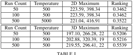
with large absolute values outweighing another criterion with smaller absolute values. Rows 2-4 of Table I show the best results obtained for this scenario using the SMOSA algorithm. Column 3 shows the normalised maximum values obtained for the optimisation criteria. Column 4 shows a scalar normalised value calculated to enable a direct comparison between the results.

The number of sensor invocations required to produce these results was recorded. The best result was obtained at a mean cost of 71,712 sensor invocations. However a very close value was obtained over 50 runs at a temperature of 500 using only 7118 sensor invocations. For this scenario, careful tuning can result in a 90% reduction in cost, as measured in sensor invocations, with only a slight degradation in algorithm performance.

Run Count Temperature 2D Maximum Ranking 50 500 223.59, 398.34 0.3462 100 500 223.59, 398.34 0.3462 500 5000 221.04, 416.91 0.3522 Run Count Temperature 3D Maximum Ranking

[image:8.612.321.555.68.218.2]

50 500 197.10, 266.28, 22 0.5206 100 500 202.88, 320.39, 19 0.5216 500 500 219.55, 296.41, 22 0.5539

TABLE I

SCENARIO CONTROL UNIT PERFORMANCE.

B. Development Effort

The following approach was used to measure the impact of the programming model on the development effort associated with the scenario. The lines of code (LOC) provided by the domain and planning expert were recorded. The size of the spatial query set produced by the automated transformations was recorded and used as a proxy measure for the development effort provided by the transformation engine. The scenario requirements were then extended to include a requirement to also display CCTV camera streams at junctions where

140

160 180

200 220

260 280 300 320

340 360 380 400

420 8

10 12 14 16 18 20 22 24

Number of Emergency Vehicles

"500r_500t" "normalised_max"

Degree of Interest

[image:8.612.67.284.470.559.2]

Maximal Distance in kms 8 10 12 14 16 18 20 22 24

Fig. 6. Extended scenario SMOSA performance for 500 runs.

emergency service vehicles are present, resulting in a three-dimensional optimisation problem. Additional layer 3 system-states were defined to detect and count the number of emer-gency service vehicles at junctions associated with selected sets of CCTV cameras and the LOC metric was measured for the extended domain and planning expert development (DM and PL respectively). The transformations were re-run and the increase in size of the spatial query data produced recorded. The ratio of increased domain and planning devel-opment effort in LOC was then compared to the ratio of the increase of spatial query data generated. This value is referred to as the “degree of automation” and calculated as:

δ(DM+P L)/ δ(P lanning M odel Size).

Specifying the additional functionality increased the size of the domain modelling effort by c. 40% from 284 to 390 LOC. The SMOSA implementation and mapping was 400 LOC. However there was no additional planning development effort required as the SMOSA algorithm mapping logic is

unchanged. The increase in development effortδ(DM+P L)

was 684/790 LOC = 15%. The spatial query set generated by the transformation engine from the original domain model was 69 KB in size. This increased to 118KB in size for the extended domain model. The degree of automation measure

for the extended scenario was: 684/790 : 69/118, i.e., a

15% increase in development effort was translated by the tool-chain into a 71% increase in application functionality as measured by the size of generated spatial query data. The increased functionality was mirrored in evaluation logs that show the original SMOSA control units performed 7118 sensor invocations over 50 runs while the extended SMOSA control units performed 8823 sensor invocations over 50 runs, an increase of c. 24%.

(9)

algorithm using a temperature of 500 over 500 runs using the extended scenario domain model. However, the best result normalised at 0.5539 is only 6% fitter than the 0.5206 result achieved after 50 runs. The optimal result is obtained at a mean cost of 89,276 sensor invocations whereas 50 runs produced useful values after only 8823 sensor invocations, illustrating again the sensitivity of algorithm performance to parameter tuning.

The evaluation provides an indication that our approach can reduce development effort through the provision of high-level abstractions and automated code generation. This result, while pertinent primarily to the scenario, provides encouragement and motivates further testing of the programming model.

VI. RELATEDWORK

As evidenced in [10] and [11], there is a growing interest in applying model-driven techniques in pervasive computing environments for purposes such as managing heterogeneity of devices, masking the complexity of dynamic environments, and promoting code reuse. [12] proposes a planning-based approach to supporting autonomic computing in pervasive computing environments that allows users to specify their goals in a high-level manner and allow the planning framework to generate a plan. However the support provided in the form of automated transformations and code generation is generally immature, while the modelling languages used by these ap-proaches are often predicate based and non-intuitive to use. We identified no work relating to facilitating the development of planning and optimisation algorithms for pervasive computing environments.

Planning techniques have also been applied in complex service oriented computing domains. [13] presents an approach using planning techniques to address automatic web service composition, while [14] presents a web-service request lan-guage and a planning architecture that interleaves planning and execution to allow users to express their goals in complex business domains.

Systems such as GPT and mGPT [15] from the automated planning community address real-world planning problems and allow partially observable and dynamic planning problems to be modelled and solved theoretically using the PDDL predicate-based language. Our approach is intended to com-plement the work of the automated planning community, but our focus is on generating application code instead of plans. When executed, the code is expected to provide application functionality as specified using the domain model and policy.

VII. CONCLUSIONS

This paper has presented a model-driven approach to apply-ing plannapply-ing and optimisation algorithms in pervasive com-puting applications. The design of the programming model combines techniques from the disciplines of software engi-neering and automated planning. The evaluation demonstrates evidence of reduced development effort in a case study repre-sentative of the target class of applications. However the sen-sitivity of algorithm performance to parameter customisation,

highlights the importance of control tuning to ensure useful yet cost effective algorithm performance and presents an obstacle to completely automating the application of planning and optimisation algorithms. Layer 4 of the domain model can be used to tune parameters, while the automated transformations facilitate the rapid testing of a range of algorithms.

The planning and optimisation functionality provided by our approach can be extended by defining mappings from the planning model components to new algorithm implementa-tions. The current domain model design contains a number of assumptions that limit the scope of our approach. The design assumes that actions and transitions occur in implicit time and does not provide a way to represent events not associated with sensor readings or actuator actions and so cannot be used to model the internal dynamics of an environment. However, the domain model can be used to model partially observable environments and online algorithms can be used to react to dynamism in the environment. Current work is focused on testing the programming model on a range of optimisation and planning problems and on investigating additional domain model abstractions to allow more complex application state-space models and policies to be represented.

ACKNOWLEDGEMENT

The work described in this paper was partly supported by Science Foundation Ireland under Investigator award 02/IN1/I250 between 2003 and 2007 and grant 03/CE2/I30 1 to Lero - The Irish Software Engineering Research Center.

REFERENCES

[1] J. Spall,Introduction to Stochastic Search and Optimization. Wiley InterScience, 2003.

[2] M. Ghallab, D. Nauet al.,Automated Planning. Morgan Kaufmann, 2004.

[3] A. Harrington and V. Cahill, “Domain modelling for ubiquitous com-puting applications,”AINA Workshop, vol. 2, pp. 326–333, 2007. [4] M. Rom´an, C. Hess et al., “A middleware infrastructure for active

spaces,”IEEE Pervasive Computing, vol. 1, no. 4, pp. 74–83, 2002. [5] D. Nicklas, M. Grossmannet al., “Nexusscout: an advanced

location-based application on a distributed, open mediation platform,” inVLDB. VLDB Endowment, 2003, pp. 1089–1092.

[6] IEEE, “Ieee standard for a smart transducer interface for sensors and actuators wireless communication protocols and transducer electronic data sheet (teds) formats,”IEEE Std 1451.5-2007, pp. C1 –236. [7] J. Barnett, R. Akolkaret al., “State chart xml: State machine notation

for control abstraction,” W3C Working Draft, 2009.

[8] L. Klein,Sensor Technologies and Data Requirements for ITS. Artech House, 2001.

[9] B. Suman and P. Kumar, “A survey of simulated annealing as a tool for single and multiobjective optimization,”Journal of the Operational Research Society, no. 57, pp. 1143–1160, 2006.

[10] L. Baresi and et al, “Towards a model-driven approach to develop applications based on physical active objects,” inAPSEC ’06, 2006. [11] E. Serral, P. Valderas et al., “Towards the model driven development

of context-aware pervasive systems,”Pervasive and Mobile Computing, July 2009.

[12] A. Ranganathan, “Autonomic pervasive computing based on planning,” inICAC 04. IEEE Computer Society, 2004, pp. 80–87.

[13] P. Traverso and M. Pistore, “Automated composition of semantic web services into executable processes,” inThe Semantic Web ISWC 2004. Springer Berlin / Heidelberg, 2004, vol. 3298, pp. 380–394.