Proceedings of NAACL-HLT 2018, pages 506–515
Neural Tensor Networks with Diagonal Slice Matrices
Takahiro Ishihara1 Katsuhiko Hayashi2 Hitoshi Manabe1 Masahi Shimbo1 Masaaki Nagata3
1 Nara Institute of Science and Technology 2 Osaka University
3 NTT Communication Science Laboratories
1{ishihara.takahiro.in0, manabe.hitoshi.me0, shimbo}@is.naist.jp
2 [email protected] 3 [email protected]
Abstract
Although neural tensor networks (NTNs) have been successful in many natural language pro-cessing tasks, they require a large number of parameters to be estimated, which often results in overfitting and long training times. We ad-dress these issues by applying eigendecompo-sition to each slice matrix of a tensor to reduce the number of parameters. We evaluate our proposed NTN models in two tasks. First, the proposed models are evaluated in a knowledge graph completion task. Second, a recursive NTN (RNTN) extension of the proposed mod-els is evaluated on a logical reasoning task. The experimental results show that our pro-posed models learn better and faster than the original (R)NTNs.
1 Introduction
Alongside the nonlinear activation functions, lin-ear mapping by matrix multiplication is an es-sential component of neural network (NN) mod-els, as it determines the feature interaction and thus the expressiveness of models. In addition to the matrix-based mapping, neural tensor net-works (NTNs) (Socher et al.,2013a) employ a 3-dimensional tensor to capture direct interactions among input features. Due to the large expres-sive capacity of 3D tensors, NTNs have been suc-cessful in an array of natural language process-ing (NLP) and machine learnprocess-ing tasks, includ-ing knowledge graph completion (KGC) (Socher et al., 2013a), sentiment analysis (Socher et al.,
2013b), and reasoning with logical semantics (Bowman et al.,2015). However, since a 3D ten-sor has a large number of parameters, NTNs need longer time to train than other NN models. More-over, the millions of parameters often make the model suffer from overfitting (Yang et al.,2015).
To solve these problems, we propose two new parameter reduction techniques for NTNs. These
techniques drastically decrease the number of pa-rameters in an NTN without diminishing its ex-pressiveness. We use the matrix decomposition techniques that are utilized for KGC inYang et al.
(2015) and Trouillon et al. (2016). Yang et al.
(2015) imposed a constraint that a matrix in the bilinear term in their model had to be diagonal. As mentioned in a subsequent section, this is es-sentially equal to assuming that the matrix be symmetric and performing eigendecomposition.
Trouillon et al. (2016) also applied eigendecom-position to a matrix by regarding it as the real part of a normal matrix. Following these studies, we perform simultaneous diagonalization on all slice matrices of a NTN tensor. As a result, mapping by a 3D (n×n×k) tensor is replaced with an array ofk“triple inner products” of two input vec-tors and a weight vector. Thus, we obtain two new NTN models where the number of parameters is reduced fromO(n2k)toO(nk).
On a KGC task, these parameter-reduced NTNs (NTN-Diag and NTN-Comp) alleviate overfitting and outperform the original NTN. Moreover, our proposed NTNs can learn faster than the original NTN. We also show that our proposed models per-form better and learn faster in a recursive setting by examining a logical reasoning task.
2 Background
We consider mapping in a neural network (NN) layer that takes two vectors as input, such as recursive neural networks. Recurrent neural networks also has this structure, with one input vector being the hidden state from the previous time step. As a mapping before activation in the NN layer, linear mapping (matrix multiplication) is commonly used:
W1x1+W2x2 = [W1,W2]
[
x1 x2
]
=W x.
Here, sincex1,x2 ∈ Rn,W1,W2 ∈ Rk×n, this linear mapping is a transformation from R2n to Rk. Linear mapping, which is a standard
com-ponent of NNs, has been applied successfully in many tasks. However, it cannot consider the teraction between different components of two in-put vectors, which renders it not ideal for model-ing complex compositional structures such as trees and graphs.
To alleviate this problem, some models such as NTNs (Socher et al.,2013a) have explored 3D ten-sors to yield more expressive mapping:
xT1W[1:k]x2 =
xT
1W[1]x2 xT
1W[2]x2 ... xT1W[k]x2
=
sum(W[1]⊙(x1⊗x2)
)
sum(W[2]⊙(x1⊗x2)
)
... sum(W[k]⊙(x
1⊗x2))
whereW[1:k]∈Rn×n×k. The output of this
map-ping is an array ofkbilinear products in the form of xT1W[i]x2. Thus, this is also a transforma-tion from R2n to Rk. Each element of the
out-put of this mapping equals the sum of W[i] ⊙ (x1⊗x2), where⊙and⊗represent, respectively, the Hadamard and the outer products. Hence this mapping captures the direct interaction between different components (or “features”) in two input vectors. Thanks to this expressiveness, NTNs are effective in tasks such as knowledge graph com-pletion (Socher et al., 2013a), sentiment analy-sis (Socher et al., 2013b), and logical reasoning (Bowman et al.,2015).
Although mapping by a 3D tensor provides ex-pressiveness, it has a large number (O(n2k)) of parameters. Due to this, NTNs often suffer from overfitting and long training times.
3 Matrix Decomposition
3.1 Simple Matrix Decomposition (SMD)
To reduce the number of parameters of a slice matrix W[i] ∈ Rn×n in a tensor, simple
ma-trix decomposition (SMD) is commonly used (Bai et al., 2009). SMD factorizesW[i] into a prod-uct of two low rank matrices S[i] ∈ Rn×m and
T[i]∈Rm×n(m≪n):
W[i]≃S[i]T[i]. (1)
By plugging (1) into bilinear termxT
1W[i]x2, we obtain the approximationxT1S[i]T[i]x2. SMD re-duces the number of parameters ofW[i] fromn2 to2nm. However, the dimensionmforS andT is a hyperparameter and must be determined prior to training.
3.2 Simultaneous Diagonalization
This section introduces two techniques that can simultaneously diagonalize all slice matrices W[1], . . . ,W[i], . . . ,W[k]∈Rn×n. As described
in (Liu et al.,2017), we make use of the fact that if matricesV[1:k]form a commuting family: i.e., V[i]V[j] = V[j]V[i], ∀i, j ∈ {1,2, . . . , k}, they can be diagonalized by a shared orthogonal or uni-tary matrix. Both of the two techniques reduce the number of parameters of W[i] toO(n) from O(n2).
3.2.1 Orthogonal Diagonalization
Many NLP datasets contain symmetric patterns. For example, if binary relation(Bob, is relative of, Alice) holds in a knowledge graph, then (Alice, is relative of, Bob) should also hold in it. En-glish phrases “dog and cat” and “cat and dog” have identical meaning. For symmetric structures, we can reasonably suppose that each slice ma-trix W[i] of a 3D tensor is symmetric because xT
1W[i]x2must equalxT2W[i]x1.
WhenW[i]∈Rn×nis symmetric, it can be
di-agonalized as:
W[i]=O[i]W[i]′O[i]T
where O[i] ∈ Rn×n is an orthogonal matrix and
W[i]′ ∈ Rn×nis a diagonal matrix. Note that an orthogonal matrix O[i] may not be equal to Oj
if i ̸= j. However, if all of the slice matrices W[1], . . . ,W[i], . . . ,W[k] ∈ Rn×n are commut-ing, we can diagonalize every slice matrix with the same orthogonal matrix O. By substitutingW[i] withOW[i]′OTinto bilinear termxT1W[i]x2, we can rewrite it as follows:
xT1W[i]x2 = xT1OW[i] ′
OTx2
= y1TW[i]′y2
= ⟨y1,w[i],y2⟩ (2)
where y1 = OTx1, y2 = OTx2, w[i] = diag(W[i]′) ∈ Rn and⟨a,b,c⟩denotes a “triple
inner product” defined by⟨a,b,c⟩=∑nl=1alblcl.
3.2.2 Unitary Diagonalization
Since most of the structures in the NLP data are not symmetric, the symmetric matrix assumption is usually violated. To obtain more expressive di-agonal matrix, we regard each slice matrixW[i]as the real part of a complex matrix and consider its eigendecomposition.
For any real matrixW[i], there exists a complex normal matrix Z[i] whose real part is equal to it: W[i] = ℜ(Z[i]). ℜ(·) represents an operation that takes the real part of a complex number, vec-tor or matrix. Further, any complex normal ma-trix can be diagonalized by a unitary mama-trix. With these two properties, any real matrixW[i]can be diagonalized as follows (Trouillon et al.,2016):
W[i]=ℜ(Z[i])=ℜ(U[i]Z[i]′U[i]∗).
Here, U[i] ∈ Cn×n is a unitary matrix, Z[i]′ ∈
Cn×n is a diagonal matrix, and U[i]∗ is the con-jugate transpose of U[i]. To guarantee that ev-ery slice matrix can be diagonalized with the same unitary matrix U instead of U[i], we assume all of the normal matricesZ[1], . . . ,Z[i], . . . ,Z[k] ∈
Cn×nare commuting as in Section3.2.1.
Substituting ℜ(U Z[i]′U∗) whose U is the same unitary matrix in all slice matrices, we can rewrite every bilinear termxT
1W[i]x2as follows:
xT1W[i]x2 =ℜ
(
⟨y1,w[i],y2⟩
)
=⟨ℜ(y1),ℜ(w[i]),ℜ(y2)⟩ +⟨ℜ(y1),ℑ(w[i]),ℑ(y2)⟩ +⟨ℑ(y1),ℜ(w[i]),ℑ(y2)⟩
− ⟨ℑ(y1),ℑ(w[i]),ℜ(y2)⟩, (3)
where y1 = UTx1, y2 = U∗x2, w[i] = diag(Z[i]′) ∈ Cn, and⟨y
1,w[i],y2⟩ is the triple Hermitian inner product of y1, w[i] and y
2 de-fined by⟨a,b,c⟩ = ∑nl=1alblcl. This technique
reduces the number of parameters of the matrices from n2 to 2n. As shown in the right-hand side of Eq. (3),ℜ(⟨y1,w[i],y2⟩
)
can be replaced with three additions and a subtraction of the triple inner product of real vectors.
4 Neural Network Models
This section introduces the baseline and our pro-posed models. After describing them, we explain how to extend them for handling compositional structures like binary trees.
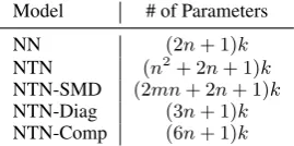
Model # of Parameters
NN (2n+ 1)k
[image:3.595.349.484.62.129.2]NTN (n2+ 2n+ 1)k NTN-SMD (2mn+ 2n+ 1)k NTN-Diag (3n+ 1)k NTN-Comp (6n+ 1)k
Table 1: Comparison of the number of parameters among the models
4.1 Baseline Models Neural Network (NN)
First, we describe a standard single layer neural network (NN) model for two vectorsx1,x2∈Rn.
The model uses linear mapping V ∈ Rk×2n to
combine two input vectors:
f(V
[
x1 x2
]
+b)
whereb∈Rkis a bias term andf is a non-linear
activation function. The NN model has only(2n+ 1)k parameters, and does not consider the direct interactions betweenx1andx2.
Neural Tensor Network (NTN)
Socher et al.(2013a) proposed a neural tensor net-work (NTN) model that uses a 3D tensorW[1:k]∈
Rn×n×kto combine two input vectors:
f(xT1W[1:k]x2+V
[
x1 x2
]
+b).
Unlike the standard NN model, NTN can directly relate two input vectors using a tensor. However, it has too many parameters;(n2+ 2n+ 1)k.
NTN-SMD
Although the NTN model has tremendous ex-pressive power, it is extremely time-consuming to compute, since a naive 3D tensor product in-curO(n2k) computation time. To overcome this weakness,Zhao et al.(2015) andLiu et al.(2015) independently introduced simple matrix decompo-sition (SMD) to the NTN model by replacing each slice matrix W[i] with its factorized approxima-tion given by Eq. (1):
f(xT1S[1:k]T[1:k]x2+V
[
x1 x2
]
+b)
where S[1:k] ∈ Rn×m×k,T[1:k] ∈ Rm×n×k.
4.2 NTNs with Diagonal Slice Matrices
In this paper, we introduce two new NTN models: NTN-Diag and NTN-Comp, both of which reduce the number of parameters in a 3D tensor more than NTN-SMD with little loss in the model’s gener-alization performance. Table 1 summarizes the number of parameters in each model.
NTN-Diag
We replace all slice matricesW[i]ofW[1:k]with the triple inner product formulation of Eq. (2) by assuming that they are symmetric and commuting. As a result, we derive the following new NTN for-mulation:
f(
⟨x1,w[1],x2⟩ ... ⟨x1,w[k],x2⟩
+V
[
x1 x2
]
+b)
wherew[i]∈Rn,∀i∈ {1,2, . . . , k}. Thus, under the symmetric and commuting matrix constraints, we regard mapping by a 3D tensor as an array ofk triple inner products. The total number of param-eters is just(3n+ 1)k.
NTN-Comp
By assuming that W[1], . . . ,W[i], . . . ,W[k] are real parts of normal matrices forming a commut-ing family, we can replace each slice matrix of a tensor term in NTN with the triple Hermitian in-ner product shown in Eq. (3):
f(
ℜ(⟨x1,w[1],x2⟩) ...
ℜ(⟨x1,w[k],x2⟩)
+ℜ
(
V
[
x1 x2
])
+b)
wherex1,x2 ∈ Cn, V ∈ Cn×nandw[i] ∈ Cn, ∀i ∈ {1,2, . . . , k}. Similar to NTN-Diag, we re-gard mapping by a 3D tensor as an array ofktriple Hermitian inner products. The total number of pa-rameters is just(6n+ 1)k. As is clear of its form, NTN-Diag is a special case of NTN-Comp whose vectorsx1,x2andw[i]are constrained to be real.
4.3 Recursive Neural Tensor Networks
We extend the above NTN models to handle positional structures. As a representative of com-positional structures, we consider a binary tree where each NTN layer computes a vector repre-sentation for a node by combining two vectors from its child nodes in the lower layer. Except for NTN-Comp, the models implement mappings
Rn → Rk so that each of their layers can receive
its lower layer’s output directly, if kequals ton. Thus, the models do not have to be modified for them. However, NTN-Comp cannot receive its lower layer’s output as it is because NTN-Comp is a mapping fromCntoRk. To solve this problem,
we setkto2nand treat the outputy′ ∈R2nas the
concatenation of vectors representing the real and imaginary parts ofy∈Cn:
ℜ(y) = (y′1,· · · , y′n), ℑ(y) = (yn′+1,· · · , y′2n).
Note that this approach is valid since Eq. (3) can actually be defined in real vector space by trans-forming the complex vectors inCninto real
vec-tors inR2n.
5 Related Work
Knowledge Graph Completion
In KGC, researchers usually design scoring func-tion Φ for the given triplet (s, r, o) to judge whether it is a fact or not. Here(s, r, o)denotes that entity s is linked to entity o by relation r. RESCAL (Nickel et al., 2011) uses eT
sWreo as
Φ, wherees,eoare entity embedding vectors and
Wr is an embedding matrix of relation r. This
bilinear operation is effective for the task, but its computational cost is high and it suffers from over-fitting. To overcome these problems, DistMult (Yang et al., 2015) adopts the triple inner prod-uct ⟨es,wr,eo⟩ as Φ, where wr is an
embed-ding vector of relationr. This solves those prob-lems, but it degrades the model’s ability to cap-ture directionality of relations, because the scor-ing function of DistMult is symmetric with re-spect tosando; i.e.,⟨es,wr,eo⟩ =⟨eo,wr,es⟩.
To reconcile the complexity and expressiveness of a model, ComplEx (Trouillon et al., 2016) uses complex vectors for entity and relation embed-dings. As scoring function Φ, they adopted the triple Hermitian inner product ℜ(⟨es,wr,eo⟩),
where eo denotes the complex conjugate of eo.
Sinceℜ(⟨es,wr,eo⟩) ̸= ℜ(⟨eo,wr,es⟩),
Com-plEx solves the expressiveness problem of Dist-Mult without full matrices as relation embed-dings. We can regard DistMult as a special case of RESCAL with a symmetric matrix constraint onWr. ComplEx is also a RESCAL variant with
Wr as the real part of a normal matrix. Our
ap-proach to reduce the number of parameters in a tensor.
NN Architectures
To give additional expressiveness power to stan-dard (R)NNs, many architectures have been pro-posed, such as LSTM (Hochreiter and Schmid-huber, 1997), GRU (Cho et al., 2014), and CNN (LeCun et al.,1998). NTN (Socher et al.,2013a) and RNTN (Socher et al., 2013b) are other such architectures. However, (R)NTNs differ in that they only add 3D tensor mapping to standard neu-ral networks. Thus, they can also be regarded as a powerful basic component of NNs because 3D tensor mapping can be applied to more compli-cated architectures such as those examples.
Parameter Reduction in NN
Several researchers reduced the number of param-eters of NNs by using specific parameter shar-ing mechanisms. Cheng et al.(2015) used circu-lant matrix mapping instead of conventional linear mapping and improved the time complexity of the matrix-vector product by using Fast Fourier Trans-formation (FFT). Circulant matrix
C(w) =
w1 wn . . . w3 w2
w2 w1 . . . w4 w3 ..
. ... ... ... ... wn−1 wn−2 . . . w1 wn
wn wn−1 . . . w2 w1
for wT = (w1, . . . , wn) can be factorized
into F−1diag(Fw)F with the Fourier matrix F. By assuming each slice matrix W[i] of W[1:k] is circulant, we get the same scoring function as that in Eq. (3); xT
1W[i]x2 = xT1 F−1diag(Fw[i])Fx2 = ℜ(⟨x′1,w[i]
′ ,x2′⟩) where x′1 = Fx1, x2′ = Fx2, and w[i]′ =
1
ndiag(Fw[i]) are complex vectors inCn. In this
sense, NTN-Comp is equivalent to NTN where slice matrices of the 3D tensor are restricted to be circulant.Hayashi and Shimbo(2017) established a more detailed proof of the equivalence.Lu et al.
(2016) employed a Toeplitz-like structured matrix, reducing parameters of LSTM.Chen et al.(2015) used a feature hashing technique to reduce param-eters in RNN. Although these techniques can also be extended to reduce the number of tensor-related parameters in NTN, the former needs FFT opera-tions; i.e., O(nlogn) computation time, and the latter’s contribution is only a reduction in memory consumption.
Dataset |E| |R| #Train #Valid #Test FB15k 14,951 1,345 483,142 50,000 59,701 WN18 40,943 18 141,442 5,000 5,000
Table 2: Dataset statistics.
6 Experiment
6.1 Knowledge Graph Completion
To evaluate their performance for link prediction on knowledge graphs, we compared our proposed methods (NTN-Diag and NTN-Comp) to baseline methods (NTN (Socher et al., 2013a) and NTN-SMD).
Task
LetE andRdenote entities and relations, respec-tively. A relational triplet, or simply a triplet, (s, r, o) is a triple with s, o ∈ E andr ∈ R. It represents a proposition that relation r holds be-tween subject entitysand object entityo. A triplet is called a fact if the proposition it denote is true. Aknowledge graph is a collection of knowledge triplets, with the understanding that all its mem-ber triplets are facts. It is called a graph because each triplet can be regarded as an edge in a di-rected graph; the vertices in this graph represent entities inE, and each edge is labeled by a relation inR. LetG be a knowledge graph, viewed as a collection of facts. Knowledge graph completion
(KGC) is the task of predicting whether unknown triplet(s′, r′, o′) ̸∈ G such thats′, o′ ∈ E, r′ ∈ R is a fact or not.
Models and Loss Function
The standard approach to KGC is to design a score functionΦ :E × R × E → Rthat assigns a large value when a triplet seems to be a fact. Socher et al.(2013a) defined it as follows.
uTrf
(
eTsWr[1:k]eo+Vr [
es
eo ]
+br )
Here, es,eo ∈ Rn are entity embeddings and
Wr,Vr,br,urare parameters for each relationr.
ur is a k-dimensional vector to map f’s output Rk to R which indicates a score. f is the
hy-perbolic tangent. To compare the performances of the baselines and proposed models, we change the mapping before an activation. For NTN-SMD, we change termeTsWr[1:k]eo toesTSr[1:k]Tr[1:k]eo. To
WN18 FB15K
MRR Hits@ MRR Hits@
model Filter Raw 1 3 10 Filter Raw 1 3 10
NN 0.111 0.106 7.0 11.7 18.3 0.259 0.165 17.9 28.1 41.7
NTN (k= 1) 0.740 0.512 67.6 78.4 85.2 0.347 0.188 24.1 39.3 55.2 NTN (k= 4) 0.754 0.530 69.3 79.5 86.3 0.380 0.198 27.1 43.0 59.2 NTN-SMD (m= 1) 0.243 0.216 15.9 26.1 40.9 0.278 0.172 19.3 30.1 44.7 NTN-SMD (m= 2) 0.224 0.199 15.1 23.8 37.2 0.298 0.177 20.7 32.7 47.8 NTN-SMD (m= 3) 0.299 0.255 20.4 32.4 49.2 0.312 0.183 21.7 34.5 49.9 NTN-SMD (m= 10) 0.533 0.413 42.2 59.4 74.5 0.333 0.188 22.8 37.5 53.8 NTN-SMD (m= 25) 0.618 0.463 52.1 67.8 80.0 0.341 0.187 23.2 38.6 55.5 NTN-Diag 0.824 0.590 74.8 89.6 92.7 0.443 0.238 31.5 51.2 68.5 NTN-Comp 0.857 0.610 80.1 90.9 93.1 0.490 0.246 36.3 56.7 71.9
[image:6.595.105.496.62.253.2]DistMult∗ 0.822 0.532 72.8 91.4 93.6 0.654 0.242 54.6 73.3 82.4 ComplEx∗ 0.941 0.587 93.6 94.5 94.7 0.692 0.242 59.9 75.9 84.0
Table 3: Mean Reciprocal Rank (MRR) and Hits@n for the models tested on WN18 and FB15k. MRR is reported in the raw and filtered settings. Hits@nmetrics are percentages of test examples that lie in the topnranked results. We report Hits@nin the filtered setting.∗Results are those in (Trouillon et al.,2016)
we assume all slice matrices of tensors among re-lations form a commuting family. The loss func-tion used to train the models is shown below:
N ∑
i=1
C ∑
c=1
max(0,1−Φ(T(i))+ Φ(Tc(i)))
+λ∥Ω∥22,
where λ∥Ω∥22 is an L2 regularization term, T(i) denotes the i-th example of training data of size N, andTc(i) is one of C randomly sampled
neg-ative examples for thei-th training example. We generated negative samples of a triplet(s, r, o)by corrupting its subject or object entity.
Experimental Setup
We used the Wordnet (WN18) and Freebase (FB15k) datasets to verify the benefits of our pro-posed methods. The dataset statistics are given in Table 2. We selected hyper-parameters based on Socher et al. (2013a) and Yang et al. (2015): For all of the models, the size of mini-batches was set to1000, the dimensionality of the entity vector to d = 100, and the regularization parameter to 0.0001; the tensor slice size was set tok = 4for all models, except NTN for which we also tested with k = 1 to see the influence of the slice size on the performance. We performed300epochs of training for Wordnet and 100 on Freebase using Adagrad (Duchi et al.,2011) with the initial learn-ing rate set to0.1.
For evaluation, we removed the subject or ob-ject entity of each test example and then replaced
it with all the entities in E. We computed the scores of these corrupted triplets and ranked them in descending order of scores. We here report the results collected in filtered and raw settings. In the filtered setting, given test example(s, r, o), we remove from the ranking all the other positive triplets that appear in either training, validation, or test dataset, whereas the raw metrics do not re-move these triplets.
Result
Experimental results are shown in Table3. We ob-serve the following:
• The performance of NN and NTNs differs considerably; Apparently, NN is inadequate for this task.
• By comparing the results of NTNs with dif-ferent slice sizes, we see thatk= 4performs better thank= 1.
• NTN-SMDs perform better than NN, but are all inferior to NTNs, although their results improved asm(the rank of decomposed ma-trices) is increased.
Conjunctive normal form ∧m i=1
ni
∨ j=1
Aij
Disjunctive normal form ∨m i=1
ni
∧ j=1
Aij
Table 4: Conjunctive and disjunctive normal forms in propositional logic. Aij is aliteral, which is a
propo-sitional variable or its negation. For example, p1 and
¬p2are literal, but not¬¬p3.
Name Symbol Set-theoretic definition
Entailment A⊏B A⊂B
Reverse entailment A⊐B A⊃B
Equivalence A≡B A=B
Alternation A|B A∩B=∅ ∧A∪B̸=D Negation A∧B A∩B=∅ ∧A∪B=D
Cover A ⌣ B A∩B̸=∅ ∧A∪B=D
[image:7.595.332.499.63.98.2]Independence A#B else
Table 5: Natural logic relations over formula pairs. A and B denote a formula in propositional logic.
we conclude that NTN-Diag is a better alter-native of NTN than NTN-SMD is, in terms of both accuracy and computational cost.
• NTN-Comp outperformed NTN-Diag, show-ing that its flexible constraint on matrices yielded additional expressiveness. However, NTN-Diag and NTN-Comp do not exceed DistMult and ComplEx, respectively, in al-most all measures.
Although not shown in the table, in this exper-iment, NTN-Diag and NTN-Comp was, respec-tively,3and1.7times as fast as NTN to train.
6.2 Logical Reasoning
To validate the performance of our proposed mod-els in a recursive neural network setting, we ex-perimentally tested them by having them solve a semantic compositionality problem in logic.
Task
This task definition basically follows Bowman et al.(2015): Given a pair of artificially generated propositional logic formulas, classify the relation between the formulas into one of the sevenbasic semantic relations of natural logic (MacCartney and Manning, 2009). Table 5shows these seven relation types. The formulas consist of propo-sitional variables, negation, and conjunction and disjunction connectives. AlthoughBowman et al.
(2015) generated formulas with no constraint on its form, we restricted them to disjunctive normal
not p3 ∧ p3
[image:7.595.108.258.65.113.2]p3 ⊏ (p3or p2) (p1or(p2or p4))) ⊐ (p2and not p4)
Table 6: Short examples of type of formulas and their relations in datasets.
P(⊐) = 0.8
(p1 or(p2or p4))vs(p2and not p4)
(p1 or(p2or p4))
p1 (p2 or p4)
p2 p4
(p2and not p4)
p2 not p4
and or
or
Softmax classifier
Comparison N(T)N layer
Composition RN(T)N layer
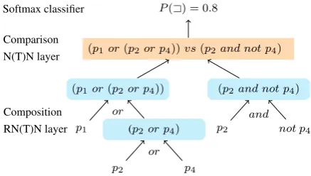
Figure 1: Comparison and composition layers. not p4 is treated as an embedding.
form (DNF) or conjunctive normal form (CNF) (Table 4). Recall that any propositional formula can be transformed into these forms.
Models and Loss Function
FollowingBowman et al.(2015), we constructed a model that infers the relations between formula pairs, as described in Table6.
The model consists of two layers: composition and comparison layers (Figure 1). The composi-tion layer outputs the embeddings of both left and right formulas by recursive neural networks. Sub-sequently, the comparison layer compares the two embeddings using a single layer neural network, and then a softmax classifier receives its output. In the composition layer, we set different parameters forandandoroperations. As a loss function, we used cross entropy with L2 regularization and ap-ply the NTNs in Section4to the comparison layer and uses RNTNs for as the composition layer.
Experimental Setup
In this experiment, an example is a pair of propo-sitional formulas, and its class label is the seven relation types between the pair. We generated examples following the protocol described in
[image:7.595.309.528.143.267.2]Model 1 2 3 4 5 6 7 8 9 10 11 12 Avg. Majority class 56.0 53.0 53.4 53.2 55.9 56.5 56.5 57.8 56.5 57.7 56.8 59.9 56.1
RNN 98.0 97.5 95.5 93.3 89.9 86.1 82.8 79.9 74.8 73.2 71.8 71.7 84.5
RNTN 99.9 99.5 98.2 95.7 92.7 88.5 84.7 81.2 78.1 77.5 74.4 74.4 87.0 RNTN-SMD(m= 1) 93.7 92.5 90.9 89.1 86.9 84.1 81.7 79.8 76.1 75.7 75.3 75.1 83.4
RNTN-SMD(m= 2) 93.0 93.4 91.7 90.3 88.2 85.5 82.7 81.4 77.6 77.0 75.4 75.8 84.3
RNTN-SMD(m= 4) 90.2 90.3 89.4 87.6 86.0 83.6 81.2 79.6 76.5 75.2 74.6 75.7 82.4
RNTN-SMD(m= 8) 86.8 84.9 83.5 82.5 81.1 79.1 76.6 75.6 72.4 71.3 70.9 71.2 77.9
RNTN-SMD(m= 16) 86.6 83.9 82.4 81.4 80.2 78.6 76.5 75.5 73.1 72.7 72.2 73.3 78.0 RNTN-Diag 99.9 98.9 98.5 97.4 94.9 91.5 87.6 85.0 80.3 78.5 77.1 75.2 88.7
RNTN-Comp 99.3 98.1 98.0 96.9 94.3 90.6 86.1 83.5 79.2 76.6 74.5 74.6 87.6
Table 7: Result of logical inference for Tests 1–12. Example in Testnhasnlogical operators in either or both left and right formulas. Each score is the average accuracy of five trials of theλthat achieved best performance on validation set. “Majority class” denotes the ratio of the majority class (relation “#”, i.e., Independence; see Table5).
Model Accuracy (Std. Dev.)
RNN 95.0 (0.8)
RNTN 97.2 (0.4)
RNTN-SMD(m= 1) 90.1 (3.4)
RNTN-SMD(m= 2) 91.4 (4.6)
RNTN-SMD(m= 4) 88.6 (7.1)
RNTN-SMD(m= 8) 82.7 (10.2)
RNTN-SMD(m= 16) 81.8 (11.7)
RNTN-Diag 98.1 (0.1)
RNTN-Comp 97.5 (0.1)
Table 8: Average accuracy and standard deviation on the validation dataset. The reported values are average over the best-performing modelλin each method.
up to12logical operators. Every formula consists of up to four variables taken from six propositional variables that are shared among all the examples. Hyperparameters and optimization are based on
Bowman et al. (2015): Embedding size d = 25 (for RNN, d = 45) and the output size of com-parison layer is k = 75, and we used AdaDelta (Zeiler,2012) for an optimizer. We searched for the best coefficientλof L2 regularization in λ∈ {0.0001,0.0003,0.0005,0.0007,0.0009,0.001}, whereasBowman et al.(2015) setλto0.001for RNN and0.0003for RNTN.
Result
The results are shown in Table7. From the table, we observe the following:
• As with KGC, the large difference in per-formance between RNN and RNTN suggests that this logical reasoning task requires fea-ture interactions to be capfea-tured1.
1Bowman (2016) also evaluated TreeLSTM, but its
ad-vantage over RNN was unclear in their experiment. For that
• RNTN-Diag achieved the best accuracy ex-cept for Tests 2 and 12 and outperformed RNTN except for Test 2. This is not surpris-ing because bothandandorare symmetric: p1 and p2 equalsp2 and p1. This matches the tensor term in RNTN-Diag which is sym-metric with respect tox1andx2.
• RNTN-Comp was the second best except for Tests 1–3 and 10–12. For all tests, its accu-racy was comparable with or superior to that of RNTN.
• RNTN-SMD (m= 1) was inferior to RNTN for most test sets, although some good re-sults were observed with m = 1,2,3 on Tests 11 and 12. Indeed, except for Tests 9– 12, RNTN-SMD (m = 1) was inferior even to RNN despite the larger number of param-eters in RNTN-SMD. RNTN-SMD (m = 2) obtained better results thanm = 1, but it is still worse than RNTN except for Tests 10-12. Further increase in m (m = 4,8,16) worsened the accuracy despite an increase of the number of parameters.
We also evaluated the stability of the model over different trials and hyperparameters. Table8
(a) Validation set.
[image:9.595.81.283.62.407.2](b) Test 12.
Figure 2: Sensitivity of accuracy toλ.
RNTN, RNTN-Diag and RNTN-Comp. This indi-cates that RNTN-SMD is a less reliable model.
RNTN-SMDs are also unstable, not only within the same λ, but also between different λs. Fig-ure 2 describes how accuracies are impacted by λs. The top graph shows validation accuracies between different λvalues. RNTN, RNTN-Diag and RNTN-Comp are stable, whereas RNN and RNTN-SMDs have steep drops. The bottom one describes the accuracies for Test 12. This also shows that RNTN-SMDs are unstable and that RNTN-Diag achieves distinctive performances.
Finally, Figure 3 shows that training times in-crease quadratically with dimension for RNTN that hasO(n2k)parameters, but not for our meth-ods, which have onlyO(nk)parameters.
7 Conclusion
We proposed two new parameter reduction meth-ods for tensors in NTNs. The first method con-strains the slice matrices to be symmetric, and the second assumes them to be normal matrices. In both methods, the number of a 3D tensor
param-Figure 3: Training times of the models.
eters is reduced fromO(n2k) toO(nk) after the constrained matrices are eigendecomposed. By re-moving the tensor’s surplus parameters, our meth-ods learn better and faster as was shown in exper-iments.2 Future work will test the versatility of
our proposals, RNTN-Diag and RNTN-Comp, in other tasks that deal with data sets exhibiting cari-ous structures.
References
Bing Bai, Jason Weston, David Grangier, Ronan Col-lobert, Kunihiko Sadamasa, Yanjun Qi, Corinna Cortes, and Mehryar Mohri. 2009. Polynomial se-mantic indexing. In Y. Bengio, D. Schuurmans, J. D. Lafferty, C. K. I. Williams, and A. Culotta, editors,
Advances in Neural Information Processing Systems 22. Curran Associates, Inc., pages 64–72.
Samuel R. Bowman. 2016. Modeling natural language semantics in learned representations. Ph.D. thesis, Stanford University.
Samuel R Bowman, Christopher Potts, and Christo-pher D Manning. 2015. Recursive neural networks can learn logical semantics. Proceedings of the 3rd Workshop on Continuous Vector Space Models and their Compositionality.
Wenlin Chen, James Wilson, Stephen Tyree, Kilian Weinberger, and Yixin Chen. 2015. Compressing neural networks with the hashing trick. In Proceed-ings of the 32nd International Conference on Ma-chine Learning. pages 2285–2294.
Yu Cheng, Felix X Yu, Rogerio S Feris, Sanjiv Kumar, Alok Choudhary, and Shi-Fu Chang. 2015. An ex-ploration of parameter redundancy in deep networks with circulant projections. In Proceedings of the IEEE International Conference on Computer Vision. pages 2857–2865.
[image:9.595.309.510.64.215.2]Kyunghyun Cho, Bart van Merrienboer, Caglar Gul-cehre, Dzmitry Bahdanau, Fethi Bougares, Holger Schwenk, and Yoshua Bengio. 2014. Learning phrase representations using rnn encoder–decoder for statistical machine translation pages 1724–1734. John Duchi, Elad Hazan, and Yoram Singer. 2011. Adaptive subgradient methods for online learning and stochastic optimization. Journal of Machine Learning Research12(Jul):2121–2159.
Katsuhiko Hayashi and Masashi Shimbo. 2017. On the equivalence of holographic and complex embed-dings for link prediction. Proceedings of the 55th Annual Meeting of the Association for Computa-tional Linguisticspages 554–559.
Sepp Hochreiter and J¨urgen Schmidhuber. 1997. Long short-term memory. Neural computation
9(8):1735–1780.
Yann LeCun, L´eon Bottou, Yoshua Bengio, and Patrick Haffner. 1998. Gradient-based learning applied to document recognition. Proceedings of the IEEE
86(11):2278–2324.
Hanxiao Liu, Yuexin Wu, and Yiming Yang. 2017. Analogical inference for multi-relational embed-dings. InProceedings of the 34th International Con-ference on Machine Learning. pages 2168–2178.
Pengfei Liu, Xipeng Qiu, and Xuanjing Huang. 2015. Learning context-sensitive word embeddings with neural tensor skip-gram model. InProceedings of the Twenty-Fourth International Joint Conference on Artificial Intelligence. pages 1284–1290.
Zhiyun Lu, Vikas Sindhwani, and Tara N Sainath. 2016. Learning compact recurrent neural net-works. InAcoustics, Speech and Signal Processing (ICASSP), 2016 IEEE International Conference on. IEEE, pages 5960–5964.
Bill MacCartney and Christopher D Manning. 2009. An extended model of natural logic. InProceedings of the eighth international conference on compu-tational semantics. Association for Computational Linguistics, pages 140–156.
Maximilian Nickel, Volker Tresp, and Hans-Peter Kriegel. 2011. A three-way model for collective learning on multi-relational data. InProceedings of the 28th international conference on machine learn-ing. pages 809–816.
Richard Socher, Danqi Chen, Christopher D Manning, and Andrew Ng. 2013a. Reasoning with neural ten-sor networks for knowledge base completion. In C. J. C. Burges, L. Bottou, M. Welling, Z. Ghahra-mani, and K. Q. Weinberger, editors, Advances in Neural Information Processing Systems 26. pages 926–934.
Richard Socher, Alex Perelygin, Jean Wu, Jason Chuang, Christopher D Manning, Andrew Ng, and Christopher Potts. 2013b. Recursive deep models
for semantic compositionality over a sentiment tree-bank. In Proceedings of the 2013 conference on empirical methods in natural language processing. pages 1631–1642.
Th´eo Trouillon, Johannes Welbl, Sebastian Riedel, ´Eric Gaussier, and Guillaume Bouchard. 2016. Complex embeddings for simple link prediction. In Proceed-ings of the 33rd International Conference on Ma-chine Learning. pages 2071–2080.
Bishan Yang, Wen-tau Yih, Xiaodong He, Jianfeng Gao, and Li Deng. 2015. Embedding entities and relations for learning and inference in knowledge bases. International Conference on Learning Rep-resentations.
Matthew D Zeiler. 2012. Adadelta: An adaptive learn-ing rate method.arXiv preprint arXiv:1212.5701. Yu Zhao, Zhiyuan Liu, and Maosong Sun. 2015.