Sentence Length
Gábor Borbély András Kornai
{borbely,kornai}@math.bme.hu
Department of Algebra, Budapest University of Technology and Economics
Abstract
The distribution of sentence length in ordi-nary language is not well captured by the ex-isting models. Here we survey previous mod-els of sentence length and present our random walk model that offers both a better fit with the data and a better understanding of the dis-tribution. We develop a generalization of KL divergence, discuss measuring the noise inher-ent in a corpus, and presinher-ent a hyperparameter-free Bayesian model comparison method that has strong conceptual ties to Minimal Descrip-tion Length modeling. The models we obtain require only a few dozen bits, orders of mag-nitude less than the naive nonparametric MDL models would.
1 Introduction
Traditionally, statistical properties of sentence length distribution were investigated with the goal of settling disputed authorship (Mendenhall,1887; Yule,1939). Simple models, such as a “monkeys and typewriters” Bernoulli process (Miller,1957) do not fit the data well, and this problem is in-herited from n-gram Markov to n-gram Hidden Markov models, such as found in standard lan-guage modeling tools like SRILM (Stolcke et al., 2011). Today, length modeling is used more often as a downstream task to probe the properties of sentence vectors (Adi et al.,2017;Conneau et al., 2018), but the problem is highly relevant in other settings as well, in particular for the current gener-ation of LSTM/GRU-based language models that generally use an ad hoc cutoff mechanism to reg-ulate sentence length. The first modern study, in-terested in the entire shape of the sentence-length distribution, isSichel(1974), who briefly summa-rizes the earlier proposals, in particular negative binomial (Yule, 1944), and lognormal (Williams, 1944), being rather critical of the latter:
The lognormal model suggested by Williams and used by Wake must be re-jected on several grounds: In the first place the number of words in a sentence constitutes a discrete variable whereas the lognormal distribution is continu-ous. Wake (1957) has pointed out that most observed log-sentence-length dis-tributions display upper tails which tend towards zero much faster than the cor-responding normal distribution. This is also evident in most of the cu-mulative percentage frequency distribu-tions of sentence-lengths plotted on log-probability paper by Williams (1970). The sweep of the curves drawn through the plotted observations is concave up-wards which means that we deal with sub-lognormal populations. In other words, most of the observed sentence-length distributions, after logarithmic transformation, are negatively skew. Fi-nally, a mathematical distribution model which cannot fit real data –as shown up by the conventionalχ2 test– cannot claim serious attention. (Sichel, 1974, p. 26)
Sichel’s own model is a mixture of Poisson dis-tributions given as
φ(r) = √
1−θγ Kγ(α
√ 1−θ)
(αθ/2)r
r! Kr+γ(α) (1)
where Kγ is the modified Bessel function of the
While Sichel’s own proposal certainly cannot be faulted on the grounds enumerated above, it still leaves something to be desired, in that the parame-tersα, γ, θare not at all transparent, and the model lacks a clear genesis. InSection 2of this article we present our own model aimed at remedying these defects and inSection 3we analyze its properties. Our results are presented isSection 4. The relation between the sentence length model and grammati-cal theory is discussed in the concludingSection 5.
2 The random walk model
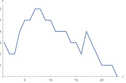
In the following Section we introduce our model of random walk(s). The predicted sentence length is basically the return time of these stochastic pro-cesses, i.e. the probability of a given length is the probability of the appropriate return time.
LetXk be a random walk onZandXk(t)the
position of the walk at time t. Let Xk(0) = k
be the initial condition. The walk is given by the following parameters:
Xk(t+ 1)−Xk(t) =
−1 with probabilityp−1
0 with probabilityp0
1 with probabilityp1
2 with probabilityp2 (2)
The random walk is the sum of these independent steps. (2) is a simple model of valency (depen-dency) tracking: at any given point we may in-troduce, with probabilityp2, some word with two open valences (e.g. a transitive verb), with proba-bilityp1 one that brings one new valence (e.g. an intransitive verb or an adjective), with probability
p0 one that doesn’t alter the count of open valen-cies (e.g. an adverbial), and with probabilityp−1 one that fills an open valency, e.g. a proper noun. For ease of presentation here we cut off at2, mak-ing no provisions for ditransitives and higher ar-ity verbs, but in actual numerical work (Section 3) we will relax this assumption. We also cut off at
−1, making no provision for those cases where a single word can fill more than one valency, as in Latinaccusativus cum infinitivoor (arguably) En-glish equi. We discuss these cutoffs further in Sec-tions3.1and5. The return time is defined as
τk= min
t≥0{t:Xk(t) = 0} (3) In particular,τ1is the time needed to go from1→
5 10 15 20 t
1 2 3 4 5 6
[image:2.595.308.515.65.201.2]k
Figure 1: Sentence length is modeled as the return time of a random walk.
0. We will calculate the probability-generating function to find the probabilities.
f(x) :=E(xτ1) (4)
The generating function ofτkeasily follows from τ1, since τk is the sum of k independent copies
ofτ1, so the generating function ofτk is simply f(x)k.
In order to calculatef(x), we condition on the first step:
f(x) =p−1·x+ finishing in one step
p0·x·f(x)+ waitτ1again
p1·x·f(x)2+ waitτ1two times
p2·x·f(x)3 waitτ1 three times (5)
Therefore, f(x) is the solution of the following equation (solved forf,xis a parameter):
p−1·x+(p0·x−1)·f+p1·x·f2+p2·x·f3 = 0 (6)
This can be solved with Cardano’s formula. The probabilities are given by
P(τk=i) = [xi]f(x)k , 1 i!
∂i ∂xif(x)
k
x=0 (7)
(Here and in what follows,[xi]refers to the coeffi-cient ofxnin the expansion of the function to the right of it.) For given parameters p−1, p0, p1, p2 andk, and a giveni, one can evaluate these prob-abilities numerically, but we need a bit more ana-lytical form. Let us define the following.
F(u) =p−1+p0·u+p1·u2+p2u3 (8)
g(f) = f
With these functions Equation 6 becomes x = g(f(x)), meaning that we are looking for the in-verse function of g. One can see that g(0) = 0
andg0(0) = 1/p−1 6= 0, therefore we can apply the Lagrange inversion theorem. Calculations de-tailed in the Appendix yield the following formula.
P(τk =i) = k i[u
i−k]Fi(u) (10)
SinceFis a polynomial, one can calculate its pow-ers by polynomial multiplication and getP(τk = i)by looking up the appropriate coefficient. Here
k is an integer (discrete) model parameter and
p−1, p0, p1, p2are real (continuous) numbers. This makes the above mentioned probabilities differen-tiablein the continuous parameters.
We call the parameterk, the starting point of the random walk, the total valency. Note thatτk ≥k
with probability1, therefore one cannot model the sentences shorter thenk. To overcome this obsta-cle, we introduce the mixture model that consists of several models with variouskvalues and coef-ficients for convex linear combination.
Pk1,α1,k2,α2,...km,αm(τ =i) =
m
X
j=1
αj·P(τkj =i)
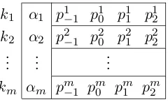
(11) where the parametersαj are mixture coefficients; positive and sum up to1, seeFigure 2. Also every term in the mixture have differentp−1, p0, p1 and
p2 values (all positive and sum up to one). In this way, we can model the sentences with length at leastminjkj.
k1 α1 p1−1 p10 p11 p12
k2 α2 p2−1 p20 p21 p22 ..
. ... ...
[image:3.595.124.244.537.610.2]km αm pm−1 pm0 pm1 pm2
Figure 2: Model parameters. The framed parameters are real, positive numbers and should sum up to1.
It is easy to generalize our model to allow higher upward steps, i.e. p3 for ditransitives or even higher steps for higher arity relations. The only technical constraint is thatp−1andp0should be positive, and no lower steps are allowed (no
p−2). This is also a reasonable assumption if a
word can only fulfill one role in a sentence, a mat-ter we return to inSection 5. Altogether, the
num-ber of upward steps is called order and it is an other hyper-parameter in our model.
Theoretically, there is no obstacle to have differ-ent number ofpvalues to differentkvalues. The model can be a heterogeneous mixture of random walks, where the individual processes can have different upward steps. But we did not investigate that possibility.
3 Model analysis
Here we introduce and analyze the experimen-tal setup that we will use in Section 4 to fit our model to various datasets. The raw data is a set of positive integers, the sentence lengths, and their corresponding weights (absolute frequen-cies) {nx}x∈X. We call n := Px∈Xnx the
size and X the support of the data. Since the model is differentiable in the continuous param-eters (including the mixing coefficients), the di-rect approach would be to perform gradient de-scent on the dissimilarity as an objective function to find the parameters. With fixed valency pa-rameterskj this is a constrained optimization task
dist(Psample,Pmodeled)→min.
In some cases, especially for smaller datasets, we might find it expedient to bin the data, for ex-ample (Adi et al., 2017) use bins (5-8), (9-12), (13-16), (17-20), (21-25), (26-29), (30-33), and (34-70). On empirical data (for English we will use the BNC1 and the UMBC Webbase2 and for other languages the SZTAKI corpus3) this partic-ular binning leaves a lot to be desired. We dis-cuss this matter in subsection 3.1, together with the choice of dissimilarity (figure of merit). An important consideration is that a high number of mixture components fit the data better but have more model parameters – this is discussed in sub-section 3.2.
3.1 Length extremes
Short utterances are common both in spoken cor-pora and in written materials, especially in dia-log intended to sound natural (see 2nd and 5th columns of Table 1). As is well known, people don’t speak in complete sentences, and a great deal of the short material is the result of sluicing, zero anaphora, and similar cross-sentence ellipsis
1
http://www.natcorp.ox.ac.uk 2
https://ebiquity.umbc.edu/resource/ html/id/351
phenomena (Merchant,2001), with complete sen-tences such as imperatives likeHelp! comprising only a small portion of the data. In nonfiction, short strings are encountered overwhelmingly in titles, subtitles, and itemized lists, material that is hard to separate from actual sentences. Here we go around the problem by permitting in the mix-ture components with low total valency (smallk
at the start of the random walk).
dataset <5 >100 dataset <5 >100 BNC-A 7.2% 0.1% Dutch 17.4% 1.1%
BNC-B 9.6% 0.1% Finnish 14.1% 0.7%
BNC-C 8.8% 0.1% Indonesian11.3% 2.0%
BNC-D 25.9% 1.4% Lithuanian25.2% 1.1%
BNC-E 8.7% 0.1% Bokmål 14.4% 1.1%
BNC-F 12.1% 0.2% Nynorsk 8.7% 0.4%
BNC-G 11.2% 0.1% Polish 23.3% 1.9%
BNC-H 14.5% 0.2% Portuguese22.7% 2.5%
BNC-J 15.2% 0.5% Romanian 8.2% 3.1%
BNC-K 29.9% 0.2% Serbian.sh 15.3% 1.9%
UMBC 3.7% 0.2% Serbian.sr 33.7% 9.0%
Catalan 15.7% 2.8% Slovak 12.4% 1.9%
Croatian16.7% 2.1% Spanish 14.7% 3.2%
Czech 13.7% 1.3% Swedish 24.6% 0.8%
[image:4.595.308.532.61.387.2]Danish 20.8% 1.1%
Table 1: Distribution of short and long sentences Especially on the long end (see columns 3 and 6 of Table 1) data becomes so sparse that some kind of binning is called for. Since the eight bins used by (Adi et al.,2017) actually ignore the very low (1-4) and very high (71+) ranges of the data, we will use ordinary deciles, setting the ten bins as the data dictates. In this regard, it is worth not-ing that in the 18 non-English corpora used in this study the low bin neglected by (Adi et al.,2017) contains on the average 17.4% of the data (vari-ance 6.3%, low 8.1% on Romanian, high 33.7% on Serbian_sr) whereas on the high end the problem is much less severe: for example in UMBC 1.0%, and in the BNC only 0.8% would be ignored.
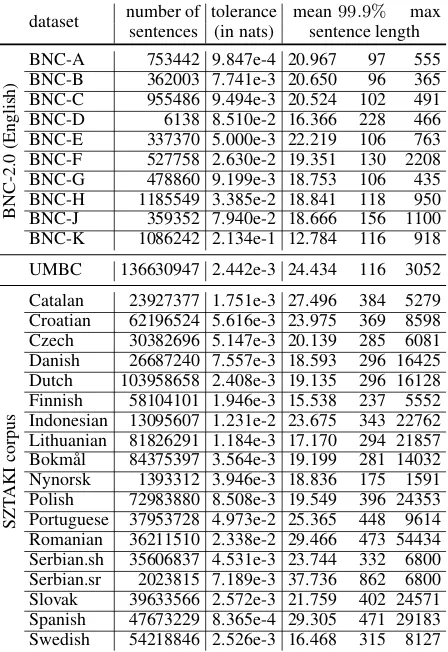
To cover 99.9% we need to consider only sen-tences up to a few hundred words (see column 5 of Table 2), and in the current study we ap-plied a cutoff of 1,000 to be above 99.9% coverage in all cases while keeping compute time manage-able. The last column ofTable 2shows the length of the longest sentence in each of the subcorpora considered. The original binning (cutoff at 71) would have resulted in coverage 95.7% on the av-erage (variance 3.1%, low 84.9% Serbian_sr, high 98.8% for Nynorsk).
The prevailing tokenization convention, where punctuation is counted as equivalent to a full word,
dataset number of sentences
tolerance (in nats)
mean99.9% max sentence length
BNC-2.0
(English)
BNC-A 753442 9.847e-4 20.967 97 555 BNC-B 362003 7.741e-3 20.650 96 365 BNC-C 955486 9.494e-3 20.524 102 491 BNC-D 6138 8.510e-2 16.366 228 466 BNC-E 337370 5.000e-3 22.219 106 763 BNC-F 527758 2.630e-2 19.351 130 2208 BNC-G 478860 9.199e-3 18.753 106 435 BNC-H 1185549 3.385e-2 18.841 118 950 BNC-J 359352 7.940e-2 18.666 156 1100 BNC-K 1086242 2.134e-1 12.784 116 918
UMBC 136630947 2.442e-3 24.434 116 3052
SZT
AKI
corpus
[image:4.595.92.271.193.366.2]Catalan 23927377 1.751e-3 27.496 384 5279 Croatian 62196524 5.616e-3 23.975 369 8598 Czech 30382696 5.147e-3 20.139 285 6081 Danish 26687240 7.557e-3 18.593 296 16425 Dutch 103958658 2.408e-3 19.135 296 16128 Finnish 58104101 1.946e-3 15.538 237 5552 Indonesian 13095607 1.231e-2 23.675 343 22762 Lithuanian 81826291 1.184e-3 17.170 294 21857 Bokmål 84375397 3.564e-3 19.199 281 14032 Nynorsk 1393312 3.946e-3 18.836 175 1591 Polish 72983880 8.508e-3 19.549 396 24353 Portuguese 37953728 4.973e-2 25.365 448 9614 Romanian 36211510 2.338e-2 29.466 473 54434 Serbian.sh 35606837 4.531e-3 23.744 332 6800 Serbian.sr 2023815 7.189e-3 37.736 862 6800 Slovak 39633566 2.572e-3 21.759 402 24571 Spanish 47673229 8.365e-4 29.305 471 29183 Swedish 54218846 2.526e-3 16.468 315 8127
Table 2: Sentence length datasets. For tolerance see subsection 3.2
has an effect on the distribution, more perceptible at the low end. Besides this (and more subtle is-sues of tokenization, such as the treatment of hy-phenation or of multiple punctuation) perhaps the most important factor influencing sentence length is morphological complexity, since in highly ag-glutinating languages a single word is sufficient for what would require a multiword sentence in English, as in Hungarianelvihetlek‘I can give you a ride’.
Since the number of datapoints is high, rang-ing from 1.3M (Nynorsk) to 136.6M (UMBC), the conventionalχ2 test does not provide a good fig-ure of merit on the original data (no fit is ever sig-nificant, especially as there is a lot of variation at the high end where only few lengths are extant), nor on the binned data, where every fit is highly significant.
pos-itive (albeit astronomically small) probabilities of arbitrarily long sentences. To remedy this defect, we define generalized KL divergence, gKL, as follows.
Definition 3.1(Motivated byTheorem A.2.). Let P and Q be probability measures over the same measurable space(X,Σ)that are both absolutely continuous with respect to a third measure dx, and letλbeP(supp(P)∩supp(Q)). Then
gKL(P,Q) :=−λ·lnλ+ Z
supp(P)∩supp(Q)
P(x)·lnP(x) Q(x)dx
(12)
Clearly, gKL reduces to the usual KL diver-gence if the support of the distributions coincide. The high end of the distribution could be ignored, at least for English, at the price of losing less than 0.1% of the data, but ignoring the short sentences, 14.4% of the BNC, is hard to countenance. As a practical matter this means we needed to bring in mixture components with total valencyk <4, and these each bring 4 parameters (the mixture weight and 3pivalues) in tow. Obviously, the more
com-ponents we use, the better the fit will be, so we need to control the trade-off between these. In sub-section 3.2 we introduce a method derived from Bayesian model comparison (MacKay,2003) that will remedy the zero modeled probabilities and an-swer the model complexity trade-off.
3.2 Bayesian model comparison
If a datasetDhas supportX, withnx > 0being the number that length x occurred, the data size is|D|=P
x∈Xnxand the observed probabilities
arepx := nx
|D|. LetHi ⊆Rdbeithmodel in some
list of models. Each model is represented by a pa-rameter vector wi ∈ Hi in the parameter space,
andsuppHi ={x|P(x| Hi)>0}is not neces-sarily equal toX. Clearly, differentHimay have
different support, but a given model has the same support for everywi. Model predictions are given
by Qwi(x) := P(x | wi,Hi), and the evidence theithmodel has is
P(Hi |D) = P
(D| Hi)·P(Hi)
P(D) (13)
If one supposes that no model is preferred over any other models (P(Hi)is constant) then the decision
simplifies to finding the model that maximizes
P(D| Hi) = Z
Hi
P(D|wi,Hi)·P(wi| Hi) dwi
(14) We make sure that no model parameter is preferred by setting a uniform prior:
P(wi | Hi) = 1/
Z
Hi
1 dwi
= 1/Vol(Hi)
(15) We estimated this integral with Laplace’s method by introducingf(wi) :=−|D1|lnQwi(D), i.e. the cross entropy (measured in nats).
P(D|wi,Hi) =
Y
x∈X
Qwi(x)
nx
f(wi) =−
X
x∈X
px·lnQwi(x) (16)
Taking −|D1|ln(•) of the evidence amounts to minimizing inithe following quantity:
f(w∗i) + 1
|D|·ln Vol(Hi)+ (17) 1
2|D|ln detf 00(w∗
i) + d 2|D|·ln
|D| 2π
where d is the dimension of Hi (number of parameters), f00 is the Hessian and w∗i = arg minwi∈Hif(wi)for a giveni. Since the the-oretical optimum of f(wi) is the entropy of the
data (ln 2·H(D)), we subtract this quantity from Equation 17so that the term f(wi) becomes the
relative entropy (measured in nats) with a theoret-ical minimum of 0.
We introduce an augmented model to deal with the datapoints whereQwi(x) = 0.
Qwi,q(x) := (
λQwi(x) ifQwi(x)>0
(1−λ)qx ifnx >0,Qwi(x) = 0 (18) where
λ= X
x∈X∩supp(Hi)
px covered probability
1−λ= X
x∈X\supp(Hi)
px uncovered probability
q and modifying Equation 17 with the auxiliary terms and subtracting the entropy of the data (ln 2· H(D)) as discussed above, one gets:
−λ·lnλ+ X
x∈X∩supp(Hi)
px·ln px Qw∗i(x)
+
1
|D|·(ln Vol(Hi) + ln Vol(aux. model)) + 1
2|D|·ln det (model Hessian) + 1
2|D|·ln det (aux. model Hessian) + d0
2|D|·ln |D|
2π (19)
where d0 is the original model dimension plus the auxiliary model dimension. One possible use (or abuse) of auxilary parameters would be to di-rectly (nonparametrically) model the low end of the length distribution. But, as we shall see in Sec-tion 4, the parametric models actually do better. To see what is going in, let us consider the asymptotic behavior of models.
For sufficiently large corpora (|D| → ∞) all but the first term will be negligible, meaning that the most precise model (in terms of gKL diver-gence) wins regardless of model size. One way out would be to choose an ‘optimum corpus size’ (Zipf,1949), a move that has already drawn strong criticism in Powers (1998) and one that would amount to little more than the addition of an ex-tra hyperparameter to be set heuristically.
Another, more data-driven approach is based on the observation that corpora have inherent noise, measurable as the KL divergence between a ran-dom subcorpus and its complement (Kornai et al., 2013) both about the same size (half the origi-nal). Here we need to take into account the fact that large sentence lengths appear with frequency 1 or 0, so subcorporaD1 andD2 = D\D1 will not have the exact same support as the original, and we need to use symmetrized gKL: the inher-ent noiseδD of a corpusDis 12(gKL(D1, D2) +
gKL(D2, D1)), where D1 andD2 are equal size subsets of the original corpusD, and the gKL di-vergence is measured on their empirical distribu-tions.
δD is largely independent of the choice of
sub-setsD1, D2of the original corpus, and can be eas-ily estimated by randomly sampled Dis. To the extent crawl data and classical corpora are
sequen-tially structured (Curran and Osborne,2002), we sometimes obtain different noise estimates based on randomDithan from comparing the first to the second half of a corpus, the procedure we followed here. In the Minimum Description Length (MDL) setting where this notion was originally developed it is obvious that we need not approximate corpora to a precision better than δ, but in the Bayesian setup that we use here matters are a bit more com-plicated.
Definition 3.2. Forδ >0let
gKLδ(P,Q) := max(0, gKL(P,Q)−δ) (20)
For a samplePwith inherent noiseδ, a modelQ is calledtolerableifgKLδ(P,Q) = 0
IfgKLδis used instead ofgKLinEquation 19
then model sizedbecomes important. If a model fits withinδ then the first term becomes zero and for large|D|values the number of model param-eters (including auxiliary paramparam-eters) will domi-nate the evidence. The limiting behavior of our ev-idence formula, with tolerance for inherent noise, is determined by the following observations:
1. Any tolerable model beats any non-tolerable one.
2. If two models are both tolerable and have dif-ferent number of model parameters (includ-ing auxiliary model), then the one with the fewer parameters wins.
3. If two models are both tolerable and have the same number of parameters, then the model volume and Hessian decides.
An interesting case is when no model can reach the inherent noise – in this case we recover the original situation where the best fit wins, no matter the model size.
4 Results
A single model Hi fit to some dataset is identi-fied by its order, defined as the number of up-ward steps the random walk can take at once:
1,2 or3, marked by the number before the first decimal; and its mixture, a non-empty subset of
withEquation 19, except thatgKLδis used with
the appropriate tolerance.
We computedwi∗with a (non-batched) gradient descent algorithm.4 We used Adagrad with ini-tial learning rate η = 0.9, starting from uniform
p and α values, and iterated until every coordi-nate of the gradient fell within ±10−3. The gra-dient descent typically took102−103iterations to reach a plateau, but about .1% of the models were more sensitive and required a smaller learning rate
η= 0.1with more (10k) iterations.
4.1 Validation
The model comparison methodology was first tested on artificially generated data. We generated 1M+1M samples of pseudo-random walks with parameters: p−1 = 0.5, p0 =p1 = 0.25 (at most one step upward) andk= 3(no mixture) and ob-tained the inherent noise and length distribution. The inherent noise was about 3.442e-4 nats. We trained all 93 models and compared them as de-scribed above.
The validation data size is 2·106 but we also replaced |D| with a hyper-parameter n in Equa-tion 19. This means that we faked the sample to be bigger (or smaller) with the same empirical distri-bution. We did this with the goal of imitating the ‘optimum corpus size’ as an adverse effect.
As seen onTable 3the true model wins. We also tested the case when the true model was simply excluded from the competing models. In this case, the tolerance is needed to ensure a stable result as
n→ ∞.
1.k3 artificial data best parameters for variousnvalues 1k 10k 100k 1M 10M 1G
with tolerance 3.k1-5 1.k3 1.k3 1.k3 1.k3 1.k3 w/o tolerance 3.k1-5 1.k3 1.k3 1.k3 1.k3 1.k3
w tolerance, -true 3.k1-5 2.k4 2.k4 2.k4 2.k4 2.k4 w/o tolerance, -true 3.k1-5 2.k4 1.k2.3 1.k2.3 1.k2.3 1.k3-5
Table 3: Optimal models for artificially generated data (1.k3) for variousnvalues.
As there are strong conceptual similarities be-tween MDL methods and the Bayesian approach (MacKay, 2003), we also compared the models with MDL, using the same locally optimal param-eters as before, but encoding them in bits. To this end we used a technique from (Kornai et al.,2013)
4You can find all of our code used for training and
evaluating at https://github.com/hlt-bme-hu/ SentenceLength
where all of the continuous model parameters are discretized on a log scale unless the discretization error exceeds the tolerance. The model with the least number of bits required wins if it fits within tolerance. (The constraints are hard-coded in this model, meaning that we re-normalized the param-eters after the discretization.) In the artificial test example, the model 1.k3 wins, which is also the winner of the Bayesian comparison. If the true model is excluded, the winner is 1.k2.3. Further MDL results will be discussed in Section4.4.
4.2 Empirical data
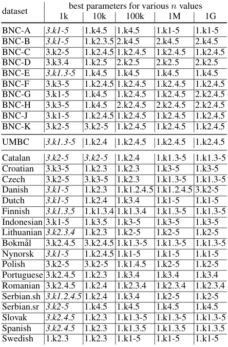
Let us now turn to the natural language corpora summarized inTable 2. Not only are the webcrawl datasets larger than the BNC sections, but they are somewhat noisier and have suspiciously long tences. To ease the computation, we excluded sen-tences longer than1,000tokens. This cutoff is al-ways well above the99.9thpercentile given in the next to last column ofTable 2. The results, sum-marized inTable 4, show several major tendencies. First, most of the models (151 out of 174) fit sentence length of the entire subcorpus better than the empirical distribution of the first half would fit the distribution of the second half. When this criterion isnotmet for the best model, i.e. the gKL distance of the model from the data is above the internal noise, the ill-fitting model form is shown initalics.
Second, this phenomenon of not achieving tol-erable fit is seen primarily (16 out of 29) in the first column ofTable 4, corresponding to a radi-cally undersampled conditionn = 1,000, and (7 out of 29) to a somewhat undersampled condition
n= 10,000.
Third, and perhaps most important, for suffi-ciently large n the Bayesian model comparison technique we advocate here actually selects rather simple models, with order 1 (no ditransitives, a matter we return to inSection 5) and only one or two mixture components. We emphasize that ‘suf-ficiently large’ is still in the realistic range, one does not have to take the limitn → ∞ to obtain the correct model. The last two columns (gigadata and infinity) always coincide, and in 21 of the 29 corpora the 1M column already yield the same re-sult.
the model comparison without usingEquation 20. Unsurprisingly, if we reward every tiny improve-ment in divergence, we get more models (159 out of 174) within the tolerable range – those outside the tolerance limit are again given in italics in Ta-ble 6. But we pay a heavy price in model complex-ity: the best models (in the last two columns) are now often second order, and we have to counte-nance a hyperparameternwhich matters (e.g. for Polish).
dataset best parameters for variousnvalues 1k 10k 100k 1M 1G ∞
BNC-A 3.k1-5 3.k2-5 1.k4.5 1.k4.5 1.k4.5 1.k4.5 BNC-B 3.k1-5 3.k1-5 1.k1.5 1.k1.5 1.k1.5 1.k1.5 BNC-C 3.k2-5 3.k2-5 3.k2-5 1.k1.4 1.k1.4 1.k1.4 BNC-D 3.k2.3.5 3.k2.3.5 3.k2.3.5 1.k2 1.k2 1.k2 BNC-E 3.k1.3-5 3.k1.3-51.k2.5 1.k2.5 1.k2.5 1.k2.5 BNC-F 3.k3.4.5 3.k3.4.5 3.k3.4.5 1.k3 1.k3 1.k3 BNC-G 3.k1-5 3.k1-5 1.k2.5 1.k2.5 1.k2.5 1.k2.5 BNC-H 3.k2.4.5 3.k3.4.5 1.k4 1.k4 1.k4 1.k4 BNC-J 3.k2.3.4 3.k2.3.4 3.k2.5 1.k2 1.k2 1.k2 BNC-K 3.k1-5 3.k1-5 1.k2 1.k2 1.k2 1.k2
UMBC 3.k1.3-5 3.k1.3-51.k2.5 1.k2.5 1.k2.5 1.k2.5
Catalan 3.k2-5 3.k2-5 1.k2.5 1.k2.5 1.k2.5 1.k2.5 Croatian 3.k3.4.5 3.k3.4.5 1.k2.5 1.k2.5 1.k2.5 1.k2.5 Czech 3.k4.5 3.k1.3.5 1.k2.5 1.k2.5 1.k2.5 1.k2.5 Danish 3.k1-5 3.k1.3.5 1.k2.5 1.k2.5 1.k2.5 1.k2.5 Dutch 3.k1-5 3.k3.4.5 1.k2.5 1.k2.5 1.k2.5 1.k2.5 Finnish 3.k1.3.5 1.k2.4 1.k2.4 1.k2.4 1.k2.4 1.k2.4 Indonesian 3.k1-5 3.k1-5 1.k2.5 1.k2.5 1.k2.5 1.k2.5 Lithuanian 3.k2.3.4 3.k2.3.4 1.k2.3 1.k2.3 1.k2.3 1.k2.3 Bokmål 3.k2.4.5 3.k2.4.5 1.k2.5 1.k2.5 1.k2.5 1.k2.5 Nynorsk 3.k1-5 1.k2.5 1.k2.5 1.k2.5 1.k2.5 1.k2.5 Polish 3.k2-5 3.k2-5 3.k2-5 3.k2-5 1.k2.5 1.k2.5 Portuguese 3.k2.3.5 3.k2.3.5 1.k2 1.k2 1.k2 1.k2 Romanian 3.k1.3-5 3.k1.3-5 1.k5 1.k5 1.k5 1.k5 Serbian.sh 3.k1.2.4.53.k2.3.5 1.k2.5 1.k2.5 1.k2.5 1.k2.5 Serbian.sr 3.k2-5 3.k2.3.4 1.k2.5 1.k2.5 1.k2.5 1.k2.5 Slovak 3.k2.4.5 3.k2-5 1.k2.5 1.k2.5 1.k2.5 1.k2.5 Spanish 3.k2.4.5 1.k2.3 1.k2.3 1.k2.3 1.k2.3 1.k2.3 Swedish 1.k2.4 1.k2.4 1.k2.4 1.k2.4 1.k2.4 1.k2.4
Table 4: Optimal models with tolerance for inner noise. Ill-fitting modelsare marked with italics.
4.3 Previous models
We also compared previous or baseline sen-tence length models with our new model. The hyper-parameters of the bins model are the bins themselves. The distribution over the bins are the continuous model-parameters. For m bins:
[1, b1),[b1, b2), . . .[bm−1,∞), the probability dis-tribution P(bi ≤ X < bi+1) = qi is to be op-timized. This model has m −1 free parameters (model dimension) and its model volume is the volume of a probabilisticm-simplex. No auxiliary model is required.
We also trained5and compared Sichel’s model (Equation 1) with our method. In this caseαandθ
are the model-parameters andγwas a non-trained hyper-parameter. InSichel(1974) it was fixedγ = −12, we trained γ ∈ {−0.5,−0.4}, the higherγ
value was usually better. Again no auxiliary model was needed.
dataset Sichel binned randwalk δ
BNC-A 3.554e-2 1.489e-2 4.409e-4 9.847e-4 BNC-B 6.212e-2 1.274e-2 7.215e-3 7.741e-3 BNC-C 4.861e-2 1.431e-2 6.989e-3 9.494e-3 BNC-D 9.917e-2 8.387e-2 5.945e-2 8.510e-2 BNC-E 6.976e-2 2.251e-2 4.353e-3 5.000e-3 BNC-F 3.153e-2 2.196e-2 2.270e-2 2.630e-2 BNC-G 2.598e-2 1.495e-2 5.762e-3 9.199e-3 BNC-H 4.765e-2 3.265e-2 3.106e-2 3.385e-2 BNC-J 3.048e-2 6.854e-2 2.946e-2 7.940e-2 BNC-K 6.583e-2 1.388e-1 3.899e-2 2.134e-1
UMBC 6.584e-2 2.615e-2 1.390e-3 2.442e-3
[image:8.595.315.517.167.489.2]Catalan 1.389e-1 6.102e-2 9.382e-4 1.751e-3 Croatian 1.131e-1 4.604e-2 2.063e-3 5.616e-3 Czech 5.857e-2 3.687e-2 2.563e-3 5.147e-3 Danish 1.618e-1 3.072e-2 2.772e-3 7.557e-3 Dutch 4.232e-1 3.447e-2 1.391e-3 2.408e-3 Finnish 9.968e-2 2.830e-2 1.659e-3 1.946e-3 Indonesian 2.159e-1 5.017e-2 1.390e-3 1.231e-2 Lithuanian - 3.113e-2 6.637e-4 1.184e-3 Bokmål - 3.332e-2 3.515e-3 3.564e-3 Nynorsk - 2.830e-2 3.757e-3 3.946e-3 Polish - 4.078e-2 1.518e-3 8.508e-3 Portuguese - 5.133e-2 4.514e-2 4.973e-2 Romanian - 6.539e-2 1.579e-2 2.338e-2 Serbian.sh - 4.676e-2 1.346e-3 4.531e-3 Serbian.sr - 1.389e-1 6.971e-3 7.189e-3 Slovak - 4.344e-2 2.184e-3 2.572e-3 Spanish - 6.501e-2 7.718e-4 8.365e-4 Swedish - 2.652e-2 2.310e-3 2.526e-3
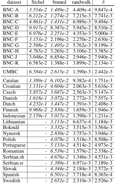
Table 5: Best of the models and their fit.Ill-fitting mod-elsare marked with italics.
As can be seen, the fit is always improved (on the average by 40%) from the mixture Poisson to the binned model, and the random walk model fur-ther improves from the binned (on the average by 70%). More important, the mixture Poisson model never, the binned model rarely, but the random walk model always approximates the data better than its inner noise. Altogether the random walk models always outperforms the other two, but not always for the same reason. In the case of bins, the fit was poor and only the fine-grained bins
per-5
formed within inherent noise. Note that none of our parametric models use mode than11 parame-ters, which makes only systems with12 or fewer bins competitive.
In case of Equation 1, Sichel already mentions that the fit is satisfactory only with binned proba-bilities, i.e. on a dumbed down distribution with 4-5 data points aggregated into one. This classic model has only2parameters, which would make it very competitive for large inherent noise or small data size, but neither is the case here.
4.4 MDL approach
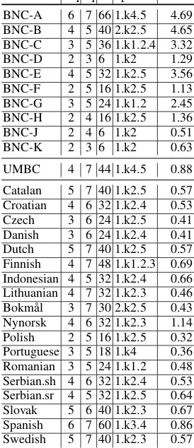
Finally, let us consider the MDL results given in Table 7. These are often (9 out of 29 subcorpora) consistent with the results obtained using Equa-tion 20, but never with those obtained without con-sidering inherent noise to be a factor. Remarkably, we never needed more than 6 bits quantization, consistent with the general principles of Google’s TPUs (Jouppi et al.,2017) and is in fact sugges-tive of an even sparser quantization regime than the eight bits employed there.
For a baseline, we discretized the naive (non-parametric) model in the same way. Not only does the quantization require on the average two bits more, but we also have to countenance a consid-erably larger number of parameters to specify the distribution within inherent noise, so that the ran-dom walk model offers a size savings of at least 95.3% (BNC-A) to 99.7% (Polish).
With the random walk model, the total number of bits required for characterizing the most com-plex distributions (66 for BNC-A and 60 for Span-ish) appears to be more related to the high consis-tency (low internal noise) of these corpora than to the complexity of the length distributions.
5 Conclusion
At the outset of the paper we criticized the stan-dard mixture Poisson length model ofEquation 1 for lack of a clear genesis – there is no obvious candidate for ‘arrivals’ or for the mixture. In con-trast, our random walk model is based on the sug-gestive idea of total valency ‘number of things you want to say’, and we see some rather clear meth-ods for probing this further.
First, we have extensive lexical data on the va-lency of individual words, and know in advance that e.g. color adjectives will be dependent on nouns, while relational nouns such as sister can
dataset best parameters for variousnvalues 1k 10k 100k 1M 1G
BNC-A 3.k1-5 1.k4.5 1.k4.5 1.k1-5 1.k1-5 BNC-B 3.k1-5 1.k2.3.5 2.k4.5 2.k4.5 2.k4.5 BNC-C 3.k2-5 1.k2.4.5 1.k2.4.5 1.k2.4.5 1.k2.4.5 BNC-D 3.k3.4 1.k2.5 2.k2.5 2.k2.5 2.k2.5 BNC-E 3.k1.3-5 1.k4.5 1.k4.5 1.k4.5 1.k4.5 BNC-F 3.k3-5 1.k2.4.5 1.k2.4.5 1.k2.4.5 1.k2.4.5 BNC-G 3.k1-5 1.k4.5 1.k2.4.5 1.k2.4.5 2.k2.4.5 BNC-H 3.k3-5 1.k4.5 2.k2.4.5 2.k2.4.5 2.k2.4.5 BNC-J 3.k1-5 1.k2.4.5 1.k2.4.5 1.k2.4.5 1.k2.4.5 BNC-K 3.k2-5 3.k2-5 1.k2.4.5 1.k2.4.5 1.k2.4.5
UMBC 3.k1.3-5 1.k2.4 1.k2.4.5 1.k2.4.5 1.k2.4.5
[image:9.595.306.528.61.399.2]Catalan 3.k2-5 3.k2-5 1.k2.4 1.k1.3-5 1.k1.3-5 Croatian 3.k3-5 1.k2.3 1.k2.3 1.k3-5 1.k3-5 Czech 3.k2-5 3.k3-5 1.k2.3 1.k1.3-5 1.k1.3-5 Danish 3.k1-5 1.k2.3 1.k1.2.4.5 1.k1.2.4.5 3.k2-5 Dutch 3.k1-5 1.k2.4 1.k3.4 1.k1-5 1.k1-5 Finnish 3.k1.3.5 1.k1.3.4 1.k1.3.4 1.k1.3-5 1.k1.3-5 Indonesian 3.k1-5 1.k3.5 1.k3-5 1.k3-5 1.k3-5 Lithuanian 3.k2.3.4 1.k2.3 1.k2-5 1.k2-5 1.k2-5 Bokmål 3.k2.4.5 3.k2.4.5 1.k1.3-5 1.k1.3-5 1.k1.3-5 Nynorsk 3.k1-5 1.k2.4.5 1.k1-5 1.k1-5 1.k1-5 Polish 3.k2-5 3.k2-5 1.k1.4.5 1.k2-5 1.k2-5 Portuguese 3.k2.4.5 1.k2.3 1.k3.4 1.k3.4 1.k3.4 Romanian 3.k2.4.5 1.k2.4 1.k2.3.4 1.k2.3.4 1.k2.3.4 Serbian.sh 3.k1.2.4.51.k2.4 1.k3.4 1.k2-5 1.k2-5 Serbian.sr 3.k2-5 1.k4.5 1.k4.5 1.k4.5 1.k4.5 Slovak 3.k2.4.5 1.k2.3 1.k1.3-5 1.k1.3-5 1.k1.3-5 Spanish 3.k2.4.5 1.k2.3 1.k1.3.5 1.k1.3.5 1.k1.3.5 Swedish 1.k2.3 1.k2.3 1.k1-5 1.k1-5 1.k1-5
Table 6: Optimal models without tolerance. Ill-fitting modelsare marked with italics.
bring further nouns or NPs. Combining the lexical knowledge with word frequency statistics is some-what complicated by the fact that a single word form may have different senses with different va-lency frames, but these cause no problems for a statistical model that convolves the two distribu-tions.
Second, thanks to Universal Dependencies6we now have access to high quality dependency tree-banks where the number of dependencies running between words w1, . . . , wk andwk+1. . . wn, the
ycoordinate of our random walk at k, can be ex-plicitly tracked. Using these treebanks, we could perform a far more detailed analysis of phrase or clause formation than we attempted here, e.g. by systematic comparison of the learned p1 and p2 values with the observable proportion of intransi-tive and transiintransi-tive verbs and relational nouns. Di-transitives are rare (in fact they usually make up less than 2% of the verbs) and we think these can be eliminated entirely (Kornai,2012) without loss
dataset mq nq tb opt % size BNC-A 6 7 66 1.k4.5 4.69 BNC-B 4 5 40 2.k2.5 4.65 BNC-C 3 5 36 1.k1.2.4 3.32 BNC-D 2 3 6 1.k2 1.29 BNC-E 4 5 32 1.k2.5 3.56 BNC-F 2 5 16 1.k2.5 1.13 BNC-G 3 5 24 1.k1.2 2.45 BNC-H 2 4 16 1.k2.5 1.36 BNC-J 2 4 6 1.k2 0.51 BNC-K 2 3 6 1.k2 0.63
UMBC 4 7 44 1.k4.5 0.88
[image:10.595.112.249.70.387.2]Catalan 5 7 40 1.k2.5 0.57 Croatian 4 6 32 1.k2.4 0.53 Czech 3 6 24 1.k2.5 0.41 Danish 3 6 24 1.k2.4 0.41 Dutch 5 7 40 1.k2.5 0.57 Finnish 4 7 48 1.k1.2.3 0.69 Indonesian 4 5 32 1.k2.4 0.66 Lithuanian 4 7 32 1.k2.3 0.46 Bokmål 3 7 30 2.k2.5 0.43 Nynorsk 4 6 32 1.k2.3 1.14 Polish 2 5 16 1.k2.5 0.32 Portuguese 3 5 18 1.k4 0.36 Romanian 3 5 24 1.k1.2 0.48 Serbian.sh 4 6 32 1.k2.4 0.53 Serbian.sr 4 5 32 1.k2.5 0.64 Slovak 5 6 40 1.k2.3 0.67 Spanish 6 7 60 1.k3.4 0.86 Swedish 5 7 40 1.k2.3 0.57
Table 7: Optimal models with MDL comparison (with tolerance). mq: Model quantization bits. nq: naive/nonparametric quantization bits. tb: total bits. opt: optimal model configuration. %size: size of ran-dom walk model as percentage of size of nonparametric model.
of generality. The same kind of analysis could be attempted for other grammatical formalisms like type-logical grammars, which make tracking the open arguments an even more attractive proposi-tion, but unfortunately these lack large parsed cor-pora. Another significant issue with formalisms other than UD is that the cross-linguistic breadth of parsed corpora is minute – do we want to base general conclusions of the type attempted here, linking predicate/argument structure to sentence length, on English alone?
Third, we can extend the analysis in a typo-logically sound manner to morphotypo-logically more complex languages. Using a morphologically an-alyzed Hungarian corpus (Oravecz et al.,2014) we measured the per-word morpheme distribution and per-sentence word distribution. We found that the random sum of ‘number of words in a sentence’ independent copies of ‘number of morphemes in a word’ estimates the per-sentence morpheme
dis-tribution within inherent noise. To the extent these results can be replicated for other morphologically complex languages (again UD morphologies7 of-fer the best testbed, though a lot remains to be done for ensuring homogeneity) problems like six-word ‘I can give you a ride’ versus one-six-word elvi-hetlekdisappear.
Another avenue of research alluded to above would be the study of subject- and object-control verbs and infinitival constructions, where single nouns or NPs can fill more than one open depen-dency. This would complicate the calculations in Equation 5in a non-trivial way. We plan to extend our mathematical model in a future work, but it should be clear from the foregoing that sentences exhibiting these phenomena are so rare as to ren-der unlikely any prospect of improving the statisti-cal model by means of accounting for these. This is not to say that control phenomena are irrelevant to grammar – but they are likely ‘within the noise’ for statistical length modeling.
One of the authors (Kornai and Tuza, 1992) already suggested that the number of dependen-cies open at any given point in the sentence must be subject to limitations of short-term memory (Miller,1956) – this may act as a reflective barrier that keeps asymptotic sentence length smaller than the pure random walk model would suggest. In particular, Bernoulli and other well-known models predict exponential decay at the high end, whereas our data shows polynomial decay proportional to
n−C, with C somewhere around 4 (in the 3−5
range). This is one area where our corpora are too small to draw reliable conclusions, but over-all we should emphasize that corpora already col-lected (and in the case of UD treebanks, already analyzed) offer a rich empirical field for studying sentence length phenomena, and the model pre-sented here makes it possible to use statistics to shed light on the underlying grammatico-semantic structure.
Acknowledgments
The presentation greatly benefited from the re-marks of the anonymous reviewers. Research partially supported by National Research, Devel-opment and Innovation Office (NKFIH) grants #120145: Deep Learning of Morphological Struc-ture and NKFIH grant #115288: Algebra and
gorithms as well as by National Excellence Pro-gramme 2018-1.2.1-NKP-00008: Exploring the Mathematical Foundations of Artificial Intelli-gence. A hardware grant from NVIDIA Corpo-ration is gratefully acknowledged. GNU parallel was used to run experiments (Tange,2011).
References
Yossi Adi, Einat Kermany, Yonatan Belinkov, Ofer Lavi, and Yoav Goldberg. 2017. Fine-grained anal-ysis of sentence embeddings using auxiliary predic-tion tasks. InProceedings of International Confer-ence on Learning Representations.
Alexis Conneau, Germán Kruszewski, Guillaume Lample, Loïc Barrault, and Marco Baroni. 2018. What you can cram into a single \$&!#* vector: Probing sentence embeddings for linguistic proper-ties. InProceedings of the 56th Annual Meeting of the Association for Computational Linguistics (Vol-ume 1: Long Papers), pages 2126–2136. Associa-tion for ComputaAssocia-tional Linguistics.
James R. Curran and Miles Osborne. 2002. A very very large corpus doesn’t always yield reliable estimates. Norman P. Jouppi, Cliff Young, Nishant Patil, David Patterson, and et. al. 2017. In-datacenter perfor-mance analysis of a tensor processing unit. In Pro-ceedings of ISCA ’17.
András Kornai. 2012. Eliminating ditransitives. In Ph. de Groote and M-J Nederhof, editors, Revised and Selected Papers from the 15th and 16th Formal Grammar Conferences, LNCS 7395, pages 243– 261. Springer.
András Kornai and Zsolt Tuza. 1992. Narrowness, pathwidth, and their application in natural language processing. Discrete Applied Mathematics, 36:87– 92.
András Kornai, Attila Zséder, and Gábor Recski. 2013. Structure learning in weighted languages. In Pro-ceedings of the 13th Meeting on the Mathematics of Language (MoL 13), pages 72–82, Sofia, Bulgaria. Association for Computational Linguistics.
David J.C. MacKay. 2003. Information Theory, Infer-ence, and Learning Algorithms. Cambridge Univer-sity Press.
T.C. Mendenhall. 1887. The characteristic curves of composition.Science, 11:237–249.
Jason Merchant. 2001.The Syntax of Silence: Sluicing, Islands, and the Theory of Ellipsis. Oxford Univer-sity Press.
George A. Miller. 1956. The magical number seven, plus or minus two: some limits on our capacity for processing information. Psychological Review, 63:81–97.
George A. Miller. 1957. Some effects of intermittent silence. American Journal of Psychology, 70:311– 314.
Csaba Oravecz, Tamás Váradi, and Bálint Sass. 2014. The Hungarian Gigaword Corpus. InProceedings of the Ninth International Conference on Language Resources and Evaluation (LREC-2014). European Language Resources Association (ELRA).
David M.W. Powers. 1998. Applications and expla-nations of Zipf’s law. In D.M. W. Powers, ed-itor, NEMLAP3/CONLL98: New methods in guage processing and Computational natural lan-guage learning, pages 151–160. ACL.
H.S. Sichel. 1974. On a distribution representing sen-tence length in written prose. Journal of the Royal Statistical Society Series A, 137(1):25–34.
Andreas Stolcke, Jing Zheng, Wen Wang, and Victor Abrash. 2011. Srilm at sixteen: Update and outlook. InProceedings of IEEE Automatic Speech Recogni-tion and Understanding Workshop, volume 5. O. Tange. 2011. Gnu parallel - the
command-line power tool. ;login: The USENIX Magazine, 36(1):42–47.
W.C. Wake. 1957. Sentence-length distributions of Greek authors. Journal of the Royal Statistical So-ciety Series A, 120:331–346.
C.B. Williams. 1944. A note on the statistical analy-sis of sentence-length as a criterion of literary style. Biometrika, 31:356–361.
G. Udny Yule. 1939. On sentence-length as a statisti-cal characteristic of style in prose: with application-sto two cases of disputed authorship. Biometrika, 30:363–390.
G. Udny Yule. 1944. The Statistical Study of Literary Vocabulary. Cambridge University Press.
George K. Zipf. 1949. Human Behavior and the Prin-ciple of Least Effort. Addison-Wesley.
A Appendix
Theorem A.1. Let us definefasx= Ff(f((xx)))with
F(0)>0, then
xi(f(x))k= k i[x
i−k]Fi(x) (21)
Proof. By Lagrange–Bürmann formula with com-position functionH(x) =xk.
Theorem A.2. In the Bayesian evidence if both the model and parameter a priori is uniform, then
P(Hi |D) = P
(D| Hi)·P(Hi)
P(D)
∝f(w∗i)+
1
n·ln Vol(Hi) + 1
2nln detf 00(w∗
i) + d 2n·ln
wheref(wi)is the cross entropy of the measured
and the modeled distributions. SeeEquation 17.
If the augmented model (18) is used, then Equa-tion 19follows.
Proof.
P(D| Hi)uniform a priori= Z
P(D|wi,Hi)· 1
Vol(Hi)dwi= 1
Vol(Hi) ·
Z Y
x∈X
Qwi(x)
nxdw
i=
Z
exp
n
−n·
f(wi)
z }| {
−X
x∈X nx
n ·lnQwi(x) !
o
dwi
Vol(Hi)
Using Laplace method:
≈ 1
Vol(Hi)·e −n·f(w∗
i)·
2π n
d2
p
detf00(w∗ i)
Taking −1
nln(•) for scaling (does not effect the
relative order of the models):
1
nln Vol(Hi) +f(w ∗ i) +
1
2nln detf 00
(w∗i)+
d 2n ·ln
n
2π
As for the augmented model, the model param-eters are the concatenation of the original parame-ters and the auxiliary parameparame-ters. Thus the overall Hessian is the block-diagonal matrix of the origi-nal and the auxiliary Hessian. Similarly, the over-all model volume is the product of the original and the auxiliary volume. Trivially, the logarithm of product is the sum of the logarithms.
Since the auxiliary model can fit the uncovered part perfectly: px= (1−λ)·qxonx /∈suppHi.
See (18) for thatλis the covered probability of the
sample.
P(D| H0i) =−
X
x∈X\supp(Hi)
px·lnpx
− X
x∈X∩supp(Hi)
px·ln λ·Qw∗
i(x)
+
1
n·(ln Vol(Hi) + ln Vol(aux. model)) + 1
2n ·ln det (model Hessian) + 1
2n·ln det (aux. model Hessian) + d0
2n·ln n
2π (22)
whered0 is the overall parameter number.
Further, if one subtracts the entropy of the sam-ple then only the first two term is changed com-pared toEquation 22andEquation 19follows.
X
x∈X
px·lnpx−
X
x∈X\supp(Hi)
px·lnpx
− X
x∈X∩supp(Hi)
px·ln λ·Qw∗
i(x)
=
X
x∈X∩supp(Hi)
px·ln px λ·Qw∗
i(x)
=
X
x∈X∩supp(Hi)
px· ln px
Qw∗i(x)
+ ln1 λ
!
=
λ·(−lnλ) + X x∈X∩supp(Hi)
px·ln px
Qw∗
i(x)