218
Twist Bytes - German Dialect Identification with Data Mining
Optimization
Fernando Benites1, Ralf Grubenmann2, Pius von D¨aniken2, Dirk von Gr¨unigen1, Jan Deriu1, and Mark Cieliebak1
1Zurich University of Applied Sciences, Switzerland 2SpinningBytes AG, Switzerland
[email protected], [email protected], [email protected], [email protected], [email protected], [email protected]
Abstract
We describe our approaches used in the German Dialect Identification (GDI) task at the VarDial Evaluation Campaign 2018. The goal was to identify to which out of four dialects spoken in German speaking part of Switzerland a sentence belonged to. We adopted two different meta-classifier approaches and used some data mining insights to improve the preprocessing and the meta-classifier parameters. Especially, we focused on using different feature extraction methods and how to combine them, since they influenced the performance very differently of the system. Our system achieved second place out of 8 teams, with a macro averaged F-1 of 64.6%. We also participated on the surprise dialect task with a multi-label approach.
1 Introduction
The German Dialect Identification (GDI) task (Zampieri et al., 2018), organized by the VarDial Evalua-tion Campaign 2018, was a continuaEvalua-tion of last year’s competiEvalua-tions (Zampieri et al., 2017). It consisted in classifying sentences into classes corresponding to different selected dialects.
In the German speaking part of Switzerland, there are many dialects which are quite different, and speakers of one dialect might even have difficulty understanding other dialects of regions not far away. The selected dialects were roughly represented by cantons Bern, Basel (Basel-Stadt and Baselland), Luzern (Luzern and Nidwalden) and Zurich. Geographically speaking, the cantons chosen to represent the dialects create roughly a square with each side of 100 kilometers. Each sentence was transcribed and annotated with the canton of the speaker.
The identification of dialect based on the script for non-standardized dialects is a difficult task. Not only it is difficult to transcribe the dialects (although there are guidelines), but the annotation process can be very subjective. This subjectivity of the annotation manifests in similar tasks such as in labelling multi-label samples (Benites, 2017). A good example, found in this competition’s dataset, was “sch¨on” and “sch¨o¨on”, both meaning beautiful and both labelled with Luzern dialect. An interesting restriction was that no additional information than the task data should be used (closed submission).
Notably this year’s competition had a special task, to predict a surprise dialect in the test set. Thus, the training data had no data on that new dialect (training set data 4 classes, test set data 5 classes). Such a task is particularly difficult because of the small amount of training data.
We describe here the approaches taken by our team Twist Bytes. We achieved second place1with one
of our approaches. The key feature of the approaches is based on the fact that we investigated the data set using data mining methods and applied feature optimization to build two different meta-classifiers.
2 Related Work
One of the focuses of VarDial has been the challenge of dialect identification. Especially important for our study are the previous and current GDI tasks (VarDial competition reports: Zampieri et al. (2017; This work is licensed under a Creative Commons Attribution 4.0 International License. License details: http:// creativecommons.org/licenses/by/4.0/.
1The ranking proposed by the organizers was more broad, since many systems achieved similar results. We achieved second
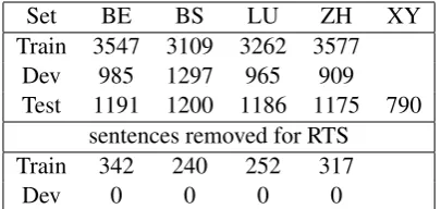
Set BE BS LU ZH XY Train 3547 3109 3262 3577
Dev 985 1297 965 909
Test 1191 1200 1186 1175 790
sentences removed for RTS
Train 342 240 252 317
[image:2.595.198.401.62.158.2]Dev 0 0 0 0
Table 1: Number of instances by Canton and Set
Zampieri et al. (2018)). Solving this problem can have a positive impact on many tasks, e.g. POS-tagging of dialectal data (Hollenstein and Aepli, 2014) and on compilation of German dialect corpora (Hollenstein and Aepli, 2015). Many studies engaged the problem in the GDI tasks, creating already a noticeable amount of related work, described in short in the competition reports. Predominantly, SVMs with different feature extraction methods performed very well.
Our approach is most similar to MAZA (Malmasi and Zampieri, 2017). MAZA uses Term Frequency on n-grams for character and unigrams for word features to train SVMs. Then it uses a Random Forest meta-classifier with 10-fold crossvalidation on the predictions of the SVMs. We additionally used Term Frequency-Inverse Document Frequency on word and, uncommonly used, on character level. We also used an SVM as meta-classifier and did not concatenate the output of the base classifiers but summed them, as will be explained in the next sections.
For the surprise task, we used a global confidence threshold which is usually a good baseline for such tasks. See (Benites, 2017) for a review on multi-label threshold strategies.
3 Methodology and Data
3.1 Task Definition
The task of GDI is, simply speaking, to classify a transcribed sentence from the ArchiMob data set (Samardˇzi´c et al., 2016) into one of four classes. Each class stands for a different canton2(Bern (BE),
Basel (BS), Luzern (LU) and Zurich (ZH)), where a different German dialect is spoken. Since the dialects are very different from standard high German, the sentences are transcribed using the guideline by Dieth (Dieth and Schmid-Cadalbert, 1986). It is a phonetics oriented transcription method but it is orthographic and partially adapted to standard German spelling habits. It uses the standard German alphabet and therefore loses some of the precision and expliciteness of phonetic transcription methods suchs as the International Phonetic Alphabet. Thus, it is not phonetic (which could give more hints about the canton) but uses a standard German script. We expect therefore that character-based and error tolerant methods will perform best, since different spellings of the same word might occur.
Although the number of speakers is clearly defined in training set (3-7 per dialect) and development set (one per dialect). There were one (BE, BS, XY) or two (LU, ZH) speakers per dialect in the test set3.
Table 1 shows the number of sentences in the training set, the development set, and test set per canton. The training set was slightly changed in comparison to the one from last year. The development set was the test set of last year’s GDI competition. The sentence distribution is almost evenly balanced over all cantons. The XY column will be discussed in Section 3.2.6 and RTS in Section 3.2.5.
3.2 System Definition
In this section, we describe our approach in detail. One part (meta crossvalidation) is based on the system from (Malmasi and Zampieri, 2017) but extended in several ways. The key improvements were focused on the data mining, specifically, the optimization of the preprocessing and feature extraction plus a preprocessing step between base classifier and meta-classifier.
2A canton is a national state in Switzerland.
We observed that much of the recognition can be performed on a character-base level, where character bigrams can provide a key insight, while demonstrating a high efficiency. The four processing steps of the system are: a) to preprocess the sentences, b) extract features from them, c) classify with a base classifier and d) pass the predictions to a meta-classifier which, in turn, provides the final prediction.
3.2.1 Preprocessing
The basic preprocessing step was to split the sentences in words by using white-spaces and convert them to lower case. No stopword removal or lemmatization was performed since these steps might erase any traces of key features for differentiating between the dialects (see (Maharjan et al., 2014)). Afterwards multiple feature extraction methods were applied.
3.2.2 Feature Extraction
We used feature extraction methods similar to (Malmasi and Zampieri, 2017), which we extended in several ways. Term Frequency (TF) with n-grams for characters and words was used for n ranging from 1 to 7. An additional preprocessing for the classifiers employed (see next section) is to normalize the TF values, at least per sentence, which in some cases can improve prediction quality. Also, we calculated the TF-IDF (Manning et al., 2008), which usually gives the best single feature set for prediction quality. For the feature extraction we mainly used the scikit-learn4 package with one modification: We also
used a custom character bigram analyzer (referred to later as CB) in order to produce character bi-grams without spaces, since the standard implementation considers all characters in the text including the spaces, especially at the beginning and end of a word. We employed TF-IDF not only on word level but also on character level.
The bm-25 measure (Jones et al., 2000) was not implemented in scikit-learn 0.19.1, therefore we used our own implementation5with the key parameter set to b=0.5.
Each of the feature extraction methods served as a separate feature set which was processed by a base classifier. The entire list: TF word n-grams (TF-W), TF character n-grams (TF-C), TF-IDF words (TF-IDF-W), customed bigrams analyzer (CB-C), TF-C normalized to 0 and 1 (TF-C-N) and TF-IDF character n-grams (TF-IDF-C).
3.2.3 Classifiers
We employed a meta classification process, where the same base classifier was trained on multiple tasks. We assessed several standard classifiers as base and meta-classifiers such as Random Forest, extreme Gradient Boosting and ARAM (Tan, 1995), and we achieved the best results with SVMs. We chose the standard implementation of scikit-learn for linear Support Vector Machines (SVMs)(Fan et al., 2008) as base classifier. It performs particularly well on large sparse feature sets, such as text classification with TF-IDF.
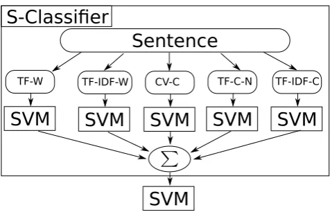
We tried concatenating all extracted features into one feature vector for a single SVM classifier, how-ever, the performance decreased in this setting (see Section 4.1 for more information). Instead, we used thesum of the scoresassigned by each SVM (trained on separate feature sets) to each sample, and then using the maximum score per class to chose the predicted class (referred to as S-Classifier in Figure 1). This lead to an large increase in prediction quality (as discussed in Section 4.1). The possibility of weighting this sum will be explained in the next section.
3.2.4 Meta-Classifiers
We explored various ensemble architectures, and finally implemented two approaches: a meta-classifier trained on the predictions of the base classifier through crossvalidation, and a hierarchical (divide and conquer) classifier.
4http://scikit-learn.org
5The implementation was used as in
SVM
TF-IDF-W
SVM
TF-W
SVM
CV-C
SVM
TF-C-N
SVM
TF-IDF-C
Sentence
[image:4.595.180.420.42.195.2]SVM
S-Classifier
Figure 1: TB-Meta Classifier Workflow, with S-Classifier
Meta Crossvalidation Classifier We experimented with a two-tier meta-classifier bottom-up with
crossvalidation (referred as TB-Meta) to eliminate the need for parameter/weighting search. The work-flow of the system is depicted in Figure 1. First an input sentence is preprocessed, then the features are extracted it and passed to the base classifiers, one classifier per feature set. The predictions of the classi-fiers are summed (until now it is an S-Classifier), and a last classifier (meta-classifier) decides about the final label. The key challenge is how to train the meta-classifier. The system is trained in three passes. First a 10-fold crossvalidation is generated and each base classifier is trained on all four classes for each single feature set. The per-class predictions are summed (output of S-Classifier). This sum is saved for each sample of the training set.6
After the crossvalidation with the S-Classifier generated predictions for all samples of the training set, these predictions together with the true labels are used to train a new linear SVM classifier, the meta-classifier. This classifier has four input features and four classes as output. Afterwards, the base classifiers are again trained with the whole training set. The idea is to grasp which predictions are likely to be a misprediction and which class should be used instead. This is practically a counter measure to solve problems with the confusion matrix.
The second level of the procedure also ensures that the class interdiscrimination is improved. Further, each base classifier prediction is then weighted by the classifier itself. That means a weighting scheme and time-consuming parameter search is not needed anymore.
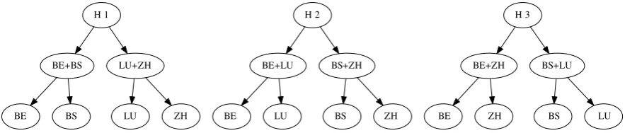
Hierarchical Classifier In cases where a confusion between two classes is frequent, one can also
apply divide and conquer approaches, especially in a binary fashion. We used a meta-label hierarchical approach (referred to as TB-Hierarchical). First an S-classifier selects between two clusters of classes (which it was trained on), and then this procedure is re-applied on the predicted cluster of classes until there is only one class left. In the four classes case of GDI 2018, there are only three possible balanced binary trees as depicted in Figure 2, referred to as H1, H2 and H3. More specifically, first the S-Classifier (with all base classifiers per feature set and summation) decides between which pair the sentence is more likely to belong to. That means the target classes of this classifier are meta classes (e.g. BS+LU). Afterwards a second S-Classifier decides which of the two cantons the sample belongs to (i.e. target classes are the actual cantons). This is a top-down approach.
In addition, we introduced an important processing step, modifying the S-Classifier. When summing the prediction of the single base classifiers, we weighted them with different values between 0 and 1 (choosing the values using a grid-search approach). For example, the prediction scores of the base classifier using TF-matrix as input feature were weighted with 0.5. We used in the competition the following weights: (TF-W:0.5, TF-IDF-W:1, CB-C:1, TF-IDF-C:0.5, TF-C:0.2).
6Although a sum is counter-intuitive, since the linear meta SVM should learn a simple summation, it seems to overfit, and
H 1
BE+BS LU+ZH
BE BS LU ZH
H 2
BE+LU BS+ZH
BE LU BS ZH
H 3
BE+ZH BS+LU
[image:5.595.78.520.66.160.2]BE ZH BS LU
Figure 2: Different combinations by divide and conquer of the labelset
3.2.5 Data Mining Optimization
Preliminary experiments showed that many errors come from the fact that many two-word sentences had different class assignments. This is not a real error as different dialects can share words and expressions. For example, the sample “ja ja” (“yes, yes”) occurred twice, and was once assigned to Zurich dialect and once to Bern. These inconsistencies make the classification more difficult, i.e. to generate a consistent model from this ambiguous data.
As a consequence, we removed one and two-word sentences from the training set, since they might decrease the performance of the model. This is the standard preprocessing of the approaches employed in this study. We will show in the experiments the impact of that step, referred to as Reduced Training Set (RTS), and differentiate to the case where all sentences are included, referred to as Complete Training Set (CTS). The affected number of sentences can be seen in Table 1. They are between 240 and 342, depending on the canton.
3.2.6 Handling Unknown Dialects
The ”Surprise Task” at GDI was to detect a previously unknown dialect. No training examples were given for this new dialect. One challenge was the small amount of training data, which makes it difficult to generate a model-discriminator for untypical samples. Number of samples of the unknown class is depicted in Table 1, referred to as XY. It has a little less samples than the other cantons.
This task is similar to multi-label problems, where a threshold must be defined up to which the con-fidence score of the classifier can be used to predict a certain label. We did a standard threshold based post-processing approach on the predictions of the meta S-Classifier. If the prediction score for every known class was too low, i.e. below the threshold, the sample belongs to the surprise dialect. The threshold was set a little lower than indecision where it was 0. We also assessed the mean and standard deviation in the development set of the prediction scores in order to make a more precise estimation.
4 Results
4.1 Performance on Development Set
We tested different combinations of the feature sets to build base classifiers, despite expecting the char-acter based feature extraction methods to perform best. We believed that because the data was relatively scarce, a multi-perspective/ensemble model was, in our view, a promising choice. Hence we trained classifiers for different feature sets and combinations. Since the number of combinations increases expo-nentially, we limited ourselves to what we expected to be the most promising combinations. The results are shown in Table 2. Basically, in the table, a base system is extended in every new line with an ad-ditional feature. The measures used are weighted and macro F-1. We also compare between RTS and CTS. In italics are those approaches that we implemented only after the competition. Marked in bold are the 6 best results, fifth and sixth best were submitted to the competition. We describe below each line in detail:
We start (#0) with a linear SVM with TF (not normalized) as feature input. Afterwards we tested instead TF-IDF (#1). Because of the No Free Lunch assumption7, we compared these two approaches
Nr/# System RTS CTS
Weighted F-1 Macro F-1 Weighted F-1 Macro F-1
- Random Baseline Dev ≈0.2500
0 SVM TF-W 0.6438 0.6524 0.6422 0.6350
1 SVM TF-IDF-W 0.6592 0.6515 0.6566 0.6497
2 RF TF-W 0.4885 0.4250 0.5100 0.4261
3 RF TF-IDF-W 0.4894 0.4228 0.5071 0.4238
4 SVM CB-C bigrams 0.6773 0.6700 0.6823 0.6739
5 same as #4 + with TF-IDF-W 0.6785 0.6687 0.6837 0.6733
6 same as #5 but CB-C n-grams 1-7 0.6785 0.6687 0.6837 0.6733
7 same as #6 + TF-IDF-C 0.6808 0.6709 0.6812 0.6713
8 same as #7 + TF-C 0.6817 0.6725 0.6830 0.6730
9 same as #8 as S-Classifier 0.6923 0.6811 0.6931 0.6829
10 same as #9 but with TF-W 0.6971 0.6878 0.6974 0.6884
11 same as #9 but with TF-W-N 0.7027 0.6929 0.7026 0.6930
12 same as #10 + bm25 0.6830 0.6751 0.6853 0.6774
13 same as #11 + bm25 0.6872 0.6786 0.6903 0.6818
14 TB-Meta 0.7010 0.6907 0.6979 0.6878
15 TB-Meta + TF-W 0.7037 0.6938 0.7015 0.6918
16 TB-Meta + bm25 0.6984 0.6904 0.6894 0.6792
17 TB-Meta + bm25 + TF-W 0.6951 0.6871 0.6932 0.6833
18 TB-Hierarchical 0.7012 0.6931 0.6976 0.6880
19 MAZA VarDial 2017 GDI winner - - 0.662
-Table 2: Per Feature System Results for the GDI Task from 2017 (using dev set). TB-Meta is Twist Bytes Meta classifier and TB-Hierarchical is Twist Bytes Hierarchical one. RF stands for random forests. CB stands for CounterVectorizer (scikit-learn TF with analyzer). Baseline random assignment (over 10 runs): weighted F-10.246±0.003, macro F-10.250±0.005
with when switching to a classifier Random Forest instead of SVM(#2-3). Then, we used the module CountVectorizer, which generates a TF matrix. However, we passed our analyzer to count character bigrams without considering white-spaces (#4). This increased F-1 scores by about 0.02. Next, method #4 was used for concatenation of TF and TF-IDF feature set but also combined with word n-grams in range 1-7 for the TF-IDF (#5). In the next line, we extended the n-grams also to the character analyzer (#6). This caused no improvement. An additional character analyzer with n-grams (range 1-7), term-weighted with TF-IDF (#7) produced a small increase. Concatenating a TF analyzer of character ngrams (range 1-7) helped to increase a little more (#8). The next line presents a considerable increase. Here, we applied the summation method and not concatenation (S-Classifier) (#9). In #10 we used TF with word n-grams in range 1-7. Since SVMs cope better with normalized values in range of [0,1], we normalized the TF values, which further increased the prediction quality (#11). Unfortunately, we did not have time to discover this until after the competition. Still, we will see that this was not best approach on the test set (but it was in the dev). We also employed bm-25, which last year’s second place was based also because it takes into account the document length. Unfortunately, this weighting scheme did not produce better results on this set (#12-13).
[image:6.595.76.545.32.351.2]BE BS LU ZH Predicted label BE BS LU ZH True label
788 190 133 80
63 953 108 76
129 558 86
48 204 132 791
Confusion Matrix 413 0.0 0.1 0.2 0.3 0.4 0.5 0.6 0.7
(a) Four Classes
BE BS LU ZH XY
Predicted label BE BS LU ZH XY True label
519 67 107 111
382
112 770 65
186 42
239 154 92
23 282
93 73 37
941 56
104 67 102
163 755 Confusion Matrix 200 400 600 800
[image:7.595.101.501.63.246.2](b) Five Classes
Figure 3: TB-Meta Confusion Matrices for GDI and Surprise Task
dev set. Notably, we see that the RTS preprocessing step consistently improved the performance of the meta-classifiers. The approaches using the CB-C always outperformed the MAZA performance of 2017.
4.2 Competition Results
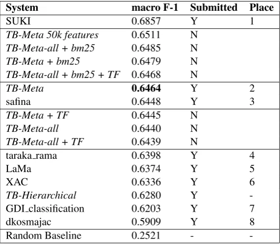
There were only 3 possible runs/submissions for each task in this year’s VarDial. This limited the number of approaches and the parameter optimization that could be done on the actual test set before the final submission. We therefore submitted the best systems from the previous section without any further opti-mization to the competition, i.e., the meta-classifier and the hierarchical classifier with the best features. The results are depicted in Table 3. The system SUKI outperforms the second best system, our TB-Meta, by around 0.04 macro F-1. We also compared in that table the approaches/parameters we optimized and investigated in depth for this study, but marked them in the column competition as N (not submitted to the competition).
From the systems not submitted, we can also see that the bm-25 feature extraction was helpful for the TB-Meta in the actual test set. It was only surpassed by controlling the maximum number of features per feature set, namely 50k features, which will be discussed in Section 4.2.1. Interestingly, using the TF features decreased the quality of the predictions.
Contrary to the previous section, TB-Hierarchical performed much worse than TB-Meta on the test set. One explanation would be that the weighting was overfitted to the development set. We did not explore all the possibilities on the test set (grid search).
The difference between RTS and CTS produced only a 0.02 points improvement in the test set; how-ever, this was enough to beat the third place by a scant. A further development was to remove all ambiguities in the training data (i.e. not only the limited by the number of words, since RTS regards only one and two word sentences). Unfortunately, this degrades the score by 0.004. This points to the fact that the ambiguities obeys a distribution for large sentences differently, decreasing the performance of the classifier.
4.2.1 Feature Number Dependency
For the competition, we used a maximum of 20000 features per subclassifier/feature set. This decision was made quite early in the process and only questioned again after the competition.
System macro F-1 Submitted Place
SUKI 0.6857 Y 1
TB-Meta 50k features 0.6511 N
TB-Meta-all + bm25 0.6485 N
TB-Meta + bm25 0.6479 N
TB-Meta-all + bm25 + TF 0.6468 N
TB-Meta 0.6464 Y 2
safina 0.6448 Y 3
TB-Meta + TF 0.6445 N
TB-Meta-all 0.6440 N
TB-Meta-all + TF 0.6439 N
taraka rama 0.6398 Y 4
LaMa 0.6374 Y 5
XAC 0.6336 Y 6
TB-Hierarchical 0.6280 Y
-GDI classification 0.6203 Y 7
dkosmajac 0.5909 Y 8
Random Baseline 0.2521 -
-Table 3: Results for the GDI task. TB-Meta is Twist Bytes Meta classifier and TB-Hierarchical is Twist Bytes Hierarchical classifier. Meta-all is Meta with Complete Training Set. Best TB-system in competition marked in bold. Submitted column states if TB-system was actually submitted to the competition. Only best submissions were placed.
0,64 0,642 0,644 0,646 0,648 0,65 0,652 0,654
10'000 20'000 50'000 100'000 150'000 200'000 300'000 1'500'000
F-1
Macr
o
[image:8.595.156.442.104.353.2]Number of Features
[image:8.595.124.477.501.694.2]Figure 5: Variations of threshold value for the confidence score to detect one of the 4 known dialects, measured in macro F-1
extracted or at least without any noticeable effect). The huge number of features comes from the fact that the analyzers using many n-grams create so many features.
4.3 Handling Unknown Dialects
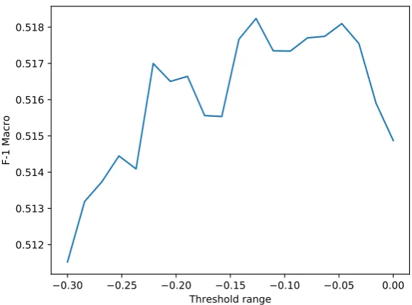
The surprise task is similar to the multi-label problems, where a threshold must be defined up to which the confidence/score of the classifier can be used to predict a certain label. We did a standard threshold based approach, i.e. we trained an SVM and when, during prediction, none of the class score exceeded the threshold, we predicted the surprise dialect. We set this threshold for the competition to -0.3 for all classes based on our qualitative assessment on the prediction of the development set. The result was a macro F-1 of 0.5115 and weighted F-1 of 0.5373. With the gold standard we investigated how the macro F-1 score varies with the threshold. The results can be seen in Figure 5 and show that a peek of 0.518 occurs around -0.12.
As can be seen from Figure 3b class XY was often mispredicted. Especially BE and LU were predicted when the true class was the XY. The difference to Figure 3b is small showing that the procedure mostly conserved the predictions. It penalized uncertain predictions, so that XY is distributed similarly as the prediction error: The good predicted class BS had small confusion with XY, where the highest confusion was with LU which had also the most predictions errors.
Also a per class optimization can be employed in this setup. Using a gridsearch over the interval -0.4 and 0.1, we achieve a macro F-1 score of 0.5230 with the following values: BE:-0.2143, BS:-0.2571, LU:-0.1286 and ZH:-0.0429.
5 Conclusion
We described our dialect identification systems that were submitted to the VarDial GDI competition. We achieved second place among 8 teams with the TB-Meta classifier system, using linear SVM as base, meta crossvalidation training, multiple word and character features. A further preprocess improved slightly the prediction quality, producing a final macro-averaged F1-score of 0.646.
References
Fernando Benites. 2017. Multi-label Classification with Multiple Class Ontologies. Ph.D. thesis, University of
Konstanz, Konstanz.
E. Dieth and C. Schmid-Cadalbert. 1986.Schwyzert¨utschi Dial¨aktschrift: Dieth-Schreibung. Lebendige Mundart.
Sauerl¨ander.
Rong-En Fan, Kai-Wei Chang, Cho-Jui Hsieh, Xiang-Rui Wang, and Chih-Jen Lin. 2008. Liblinear: A library for large linear classification. J. Mach. Learn. Res., 9:1871–1874, June.
Nora Hollenstein and No¨emi Aepli. 2014. Compilation of a Swiss German dialect corpus and its application to pos tagging. InProceedings of the First Workshop on Applying NLP Tools to Similar Languages, Varieties and Dialects, pages 85–94.
Nora Hollenstein and No¨emi Aepli. 2015. A resource for natural language processing of Swiss German dialects.
K Sparck Jones, Steve Walker, and Stephen E. Robertson. 2000. A probabilistic model of information retrieval: development and comparative experiments: Part 2. Information processing & management, 36(6):809–840.
Suraj Maharjan, Prasha Shrestha, and Thamar Solorio. 2014. A simple approach to author profiling in mapreduce. InCLEF.
Shervin Malmasi and Marcos Zampieri. 2017. German dialect identification in interview transcriptions. In
Proceedings of the Fourth Workshop on NLP for Similar Languages, Varieties and Dialects (VarDial), pages
164–169, Valencia, Spain, April.
Christopher D. Manning, Prabhakar Raghavan, and Hinrich Sch¨utze. 2008.Introduction to Information Retrieval.
Cambridge University Press, New York, NY, USA.
Tanja Samardˇzi´c, Yves Scherrer, and Elvira Glaser. 2016. ArchiMob–A corpus of spoken Swiss German. In
Proceedings of the Language Resources and Evaluation (LREC), pages 4061–4066, Portoroz, Slovenia).
Ah-Hwee Tan. 1995. Adaptive resonance associative map.Neural Networks, 8(3):437–446.
Marcos Zampieri, Shervin Malmasi, Nikola Ljubeˇsi´c, Preslav Nakov, Ahmed Ali, J¨org Tiedemann, Yves Scherrer, and No¨emi Aepli. 2017. Findings of the VarDial Evaluation Campaign 2017. InProceedings of the Fourth Workshop on NLP for Similar Languages, Varieties and Dialects (VarDial), Valencia, Spain.