connection
Stefan Vuckovic,1 Tom Irons,2Andreas Savin,3, 4 Andrew M. Teale,2and Paola Gori-Giorgi1
1)
Department of Theoretical Chemistry and Amsterdam Center for Multiscale Modeling, FEW, Vrije Universiteit, De Boelelaan 1083, 1081HV Amsterdam, The Netherlands
2)School of Chemistry, University of Nottingham, University Park, Nottingham NG7 2RD,
United Kingdom
3)
Sorbonne Universit´es, UPMC Univ Paris 06, UMR 7616, Laboratoire de Chimie Th´eorique, F-75005 Paris, France
4)CNRS, UMR 7616, Laboratoire de Chimie Th´eorique, F-75005, Paris, France
The construction of density-functional approximations is explored by modeling the adiabatic connection lo-cally, using energy densities defined in terms of the electrostatic potential of the exchange-correlation hole. These local models are more amenable to the construction of size-consistent approximations than their global counterparts. In this work we use accurate input local ingredients to assess the accuracy of range of lo-cal interpolation models against accurate exchange-correlation energy densities. The importance of the strictly-correlated electrons (SCE) functional describing the strong coupling limit is emphasized, enabling the corresponding interpolated functionals to treat strong correlation effects. In addition to exploring the performance of such models numerically for the helium and beryllium isoelectronic series and the dissociation of the hydrogen molecule, an approximate analytic model is presented for the initial slope of the local adia-batic connection. Comparisons are made with approaches based on global models and prospects for future approximations based on the local adiabatic connection are discussed.
I. INTRODUCTION
Kohn–Sham density-functional theory (KS DFT)1 is
the method most widely used in electronic structure cal-culations, due to its modest computational cost combined with an accuracy that is often competitive with much more expensive ab initio methods. The accuracy of the method is limited by the quality of approximations re-quired to describe the quantum mechanical exchange and correlation (XC) interactions of electrons. A large num-ber of density functional approximations (DFAs) for the XC–energy have been developed in recent decades.
The simplest DFAs are based on the local density ap-proximation (LDA), as proposed by KS in their 1965 paper,1 in which the XC–energy is approximated as a
functional of the density at a given point in space. The generalised gradient approximations (GGAs)2–6 go be-yond the LDA by modelling the XC–energy as a func-tional of the local density and its first derivative. The meta-GGAs7–9 are closely related but their functional
forms are also dependent on the KS kinetic energy den-sity and/or, less commonly, the Laplacian of the elec-tron density. Further developments led to the intro-duction of the occupied KS orbitals as ingredients for the XC energy (hybrid functionals,10–12 self-interaction
corrections,13–16), and more recently also the virtual KS
orbitals (double–hybrid functionals,17–19 random-phase approximations20–22). Local hybrid functionals23–26 are also an interesting alternative approach to construct hy-brid methods that are pertinent to the context of this work.
The inclusion of additional dependencies in XC– functionals has often resulted in significant improvements in their accuracy for general calculations. However, these improvements cannot be described as systematic in the
same way that the accuracy of an ab initio calculation may be systematically improved by considering a larger number of excited determinants; some DFAs give ex-cellent results for particular systems but perform very poorly otherwise, and vice versa. There also remain many problems that none of the currently available DFAs can accurately model. An important example of this, which is pertinent to this work, arestrong correlation ef-fects, commonly found in systems with near–degenerate orbitals such as the d– and f–block elements, but also in systems where chemical bonds are being broken or formed.
In the present work, the problem of constructing DFAs accurate for systems with and without strong correla-tion is examined by considering the adiabatic conneccorrela-tion (AC)27,28at the local level, i.e., in each point of space.29
The AC, discussed in subsection II A, provides an exact expression for the exchange and correlation energies by considering the changes that occur as the strength of elec-tron interaction is smoothly increased from zero. This formalism has provided the basis for the development of several DFAs,10,30–32 which attempt to interpolate the AC between the non–interacting and physical systems in order to estimate the XC–energy. An advantage of the AC formalism crucial to our construction, is that it al-lows the problem of strong correlation to be addressed in a more direct way, by creating interpolation models that are explicitly dependent on the strongly–interacting limit, in addition to the non–interacting limit, of the AC. The strongly–interacting limit of the AC has recently become the subject of much interest.29,33–37The
proper-ties of the AC integrand in this limit reveal highly non– local density dependence of correlation effects33,35,38–40
limit in DFT has focused on strictly-correlated electrons (SCE) functional, where the electrons have an infinite interaction strength. This limit is of particular inter-est from a theoretical point of view as it can be stud-ied exactly for one–dimensional systems41 and may be
closely approximated in systems with spherical or cylin-drical symmetry.33,42These studies show that in the limit of infinite interaction strength certain integrals of the density appear in the exchange-correlation functionals, revealing a mathematical structure very different from the one of the usual semi-local or orbital-dependent ap-proximations. The nonlocal radius (NLR) functional pro-posed in ref 43 approximates the SCE functional with a model that retains some of the SCE nonlocality, intro-ducing certain integrals of the spherically averaged den-sity around a reference electron. The inclusion of the NLR functional into global and local interpolations along the adiabatic connection has been very recently explored by Zhou, Bahmann and Ernzerhof.44 In another recent
work, Kong and Proynov constructed a functional com-bining the information from the Becke’13 model45 and
approximating local quantities along the AC.46
The aim of the present work is to start a systematic study of local interpolation models along the adiabatic connection, using at a first stage exact input ingredients, thus disentangling the errors due to the interpolation models from those due to the approximate ingredients. The local AC for several closed–shell atoms has been re-cently computed47 to high accuracy between the non–
interacting and physical systems using the Legendre– Fenchel formulation of DFT due to Lieb,48 and the Lieb
maximisation method of refs 49–52. Local information pertaining to the strongly–interacting limit is calculated using the SCE functional, and together these quantities are used to calculate local analogues of some established global AC interpolation functionals. We also discuss how to approximate crucial local ingredients such as the ini-tial slope of the local adiabatic curve.
In section II, relevant theoretical background is given including an overview of the AC formalism and the con-struction of DFAs from both global and local variants of the AC. Techniques for computing quantities along the AC are discussed, including the determination of the local AC as introduced in ref 47. In section II C the struction of a local model for the AC is discussed, con-sidering the non-interacting and strong-interaction limits carefully in this context. The role of the SCE in con-structing local AC interpolation models is examined. Fi-nally the forms of some local interpolation models, taken from successful existing global models are introduced. In section IV the performance of these models is assessed for the helium and beryllium isoelectronic series and for dissociation of the H2molecule, a system that typifies the
failure of present DFAs to properly account for strong– correlation. Directions for future work are outlined in section V.
II. THEORETICAL BACKGROUND
A. The Adiabatic Connection
The AC was proposed in a series of papers,27,28,53,54
which suggested that further insight into electronic cor-relations in DFT may be gained by considering a system at constant electron density as the interaction strength is smoothly scaled between zero, i.e. the KS auxiliary system, and the full physical interaction strength. This scaling of the interaction strength is achieved by the in-troduction of a simple coupling–constant coefficient λ, such that the Hamiltonian for any givenλis written as
ˆ
Hλ= ˆT+λWˆ + ˆVλ, (1) where ˆT is the kinetic energy operator, ˆW is the physical electron interaction operator and ˆVλ is the operator rep-resenting an external potentialvλthat binds the electron density atλ, such that it is always equal to the density of the physically interacting system (ρλ =ρ1, ∀λ). As
the value of λ is smoothly increased from zero to one, the system evolves adiabatically through a family ofλ– dependent wave functions Ψλ to the physical system de-scribed by Ψ1.
Given a Hamiltonian ˆHλ, one can define the corre-spondingλ–dependant universal density functional as
Fλ[ρ] = min
Ψλ→ρ
hΨλ|Tˆ+λWˆ|Ψλi (2a)
=F0[ρ] +
Z λ
0
∂Fν
∂ν dν, (2b) where eq 2b follows from the application of the Hellmann–Feynman theorem to eq 2a. This allows the well–known AC formula to be derived, yielding the fol-lowing exact expression for the XC–energy of an elec-tronic system,
Exc[ρ] =
Z 1
0
Wλ[ρ] dλ, (3)
whereWλ[ρ] is the (global) AC integrand, given by
Wλ[ρ] =hΨλ|Wˆ|Ψλi −U[ρ], (4) Ψλ[ρ] is the ground state wavefunction of ˆHλin eq 1, and U[ρ] the Hartree (Coulomb) energy.
The AC integrand may be characterized by several fea-tures that can be exactly defined: the expansion of Wλ in the non–interacting limit is given by55
Wλ[ρ] =W0[ρ] +W00[ρ]λ+. . . (λ→0), (5)
whilst its expansion in the strongly–interacting limit can be expressed as33,34,38
Wλ[ρ] =W∞[ρ] +W∞0 [ρ]λ−1/2
Here, the non–interacting terms W0[ρ] and W00[ρ] are
the exchange energy and twice the second–order corre-lation energy given by G¨orling-Levy perturbation the-ory (GL2)55,56 (see section III A 2), respectively. Their
analogues at the strongly–interacting limit, W∞[ρ] and W0
∞[ρ], have been studied in Refs. 33,34,38 and will be
discussed further in section III B. In addition to these asymptotic limits, the behaviour of Wλ under uniform coordinate scaling is also well–defined, as discussed in ref 57.
B. DFAs based on the global adiabatic connection
To construct practical DFAs one could consider mod-elling the integrand of eq 4 using a function that inter-polates between the limits of eq 5 and eq 6. The SCE limit is of particular importance in the present work, however, one could also consider models that intercept any other known point on the adiabatic connection for λ >1. Several attempts to develop DFAs based on these ideas have been put forward in the literature, see e.g. Refs. 30,31,33,34,58–62. Each form makes a choice of a simple model function and the parameters on which to base the model. These parameters often include the known exact expressions for the parameters in eq 5: W0[ρ] = Ex[{φi}], W00[ρ] = 2EcGL2[{φp, p}], since these may be computed from the set of Kohn–Sham orbitals ({φp}) and orbital energies ({p}).
The calculation of W0
0[ρ] = 2EGL2c [{φp, p}] requires
the GL2 correlation energy,55,56 which leads to a
compu-tational cost similar to the second-order Møller–Plesset (MP2) model used inab initioquantum chemistry.63The
parameters in the SCE limit entering eq 6 are clearly also of special interest in this context, and they can be computed numerically for atomic systems and molecules with cylindrical symmetry.33,42,64More frequently DFAs
are derived for points along the AC withλ >0, often by employing scaling relations to derive forms from existing DFAs. A similar strategy can also be used to approxi-mateW0
0[ρ] by a DFA, see for example ref 60.
In tandem with choosing a set of exact or approximate values to parameterize a model for the AC one must also choose an appropriate model function for the AC inte-grand. A number of these have been suggested and many have been benchmarked in practical applications. One of the simplest (and most often used) is that of a [1/1] Pad´e, as suggested by Ernzerhof.30 A range of forms were
sug-gested by Cohen et al. and tested using approximate parameterizations,60 leading to the MCY1 functional in
which a [1/1] Pad´e model is employed. Peach et al.65,66 attempted to disentangle approximations in the choice of parameters from those in the choice of model AC function by utilizing nearly exact KS orbitals and orbital energies derived from full configuration interaction data to calcu-late W0[ρ] andW00[ρ] and the corresponding interacting
wave functions to evaluateW1[ρ] via eq 4. Our present
study follows a similar philosophy, but applied to local,
rather than global, interpolations.
Seidl and co workers58,59 were the first to make use of
the strong-interaction limit (although approximated at a semilocal level, using the so-called point-charge-plus-continuum, or PC, functional) in constructing a global AC model, known as the interaction strength interpola-tion (ISI) funcinterpola-tional. The revISI model34and the models of Liu and Burke61were later constructed to take account
of theλ−1/2dependence of the second term of eq 6, which
was not correctly described by the ISI approach. Teale, Coriani and Helgaker also proposed forms for the AC in-tegrand based on the structure of traditional ab initio methodologies62and parameterized these forms to
inter-cept values of the AC at anyλ >0.
The majority of these models for the global AC suf-fer from the fact they are not size consistent in practice. This deficiency arises from a non-linear dependence on the parametersW0, W00, and a chosen approximation to
W(λ>0). When these global parameters enter in a
non-linear fashion (often as ratios) then size consistency is difficult to achieve. One route forward is to construct lo-cal AC models, which can replace these global parameters with local values defined at each point in space and may be more amenable to the construction of models that recover size-consistency (at least in the usual density-functional sense67,68).
C. Constructing a local adiabatic connection
The AC expression for the XC–energy of a system as given in eq 3 describes aglobal quantity, integrated over the coupling–constant λ. However, it may equally be written as the spatial integral of a local quantity anal-ogous to the local value of an XC–functional. To this effect, eq 3 may be re–written as
Exc[ρ] =
Z 1
0
dλ
Z
drρ(r)wλ(r), (7) where wλ(r) is the energy density at a given λ. It is well known that the energy density cannot be uniquely defined;69–71an arbitrary number of terms may be added
to wλ(r), yet an identical Wλ[ρ] recovered if their spa-tial integral is zero. Thus any such energy densities are only defined within a particulargauge, and only energy densities defined in the same gauge may be meaningfully compared.
In the context of the present work, it is both convenient and physically meaningful to definewxc,λ(r) in the gauge of the electrostatic potential of the exchange–correlation hole,
wλ(r) = 1 2
Z hλ
xc(r,r0)
|r−r0| dr
0 (8)
wherehλxc(r,r0) is the exchange–correlation hole,
hλxc(r,r0) =P λ
2(r,r0)
ρ(r) −ρ(r
andP2λ(r,r0) is the pair–density obtained from the wave function Ψλ[ρ]
P2λ(r,r0) =N(N−1)×
X
σ1...σN
Z
|Ψλ(rσ1, . . . ,rNσN)|2dr3. . .drN. (10)
The definition of energy densities in the gauge of the XC–hole is well–established in the literature, and further discussion may be found in refs 29,72,73. The coupling– constant averaged (λ–averaged) XC–energy density is de-fined as
¯ wxc(r) =
Z 1
0
wλ(r)dλ. (11) As the spatial integral of the product of this quantity and the density yields the XC–energy, the same quan-tity may be considered as a target to be modelled by XC–functionals,47 although GGAs and metaGGAs often
aim at energy densities within different definitions.5,7,72 Given the invariance of the exchange energy to electron– interaction strength, eq 11 may be trivially resolved into separate exchange and correlation terms as
¯
wc(r) = ¯wxc(r)−w¯x(r)
= ¯wxc(r)−wλ=0(r)
(12) The aim of the local interpolation schemes examined in this work is to approximate ¯wxc(r) and ¯wc(r) through
interpolating the local AC. In principle, this approach is analogous to that of the global AC interpolation schemes previously discussed, but rather than depending on quan-tities pertaining to the global AC, they are instead con-structed from their local equivalents, wλ(r). Obviously, a local interpolation will only be meaningful if all of the local terms are defined in the same gauge. It is again both convenient and logical to define all local quantities in the gauge of eq 8, as in which highly accurate energy densities wλ(r) in the range 0 ≤λ≤ 1 have previously been calculated,47and additionally can be computed for
small systems in the limitλ→ ∞.29,37
Atλ= 0, the energy density in the gauge of eq 8 is the exchange energy density w0(r) = wx(r), often denoted
x(r) in the literature (also equal to 1/2 the non-local Slater potential74), which is the crucial ingredient of
lo-cal hybrid functionals. Accurate and efficient computa-tional schemes for this quantity have become available in the recent years.26,75In a way, local interpolation models
can be viewed as local hybrids that carefully address the gauge problem.
The local equivalent of W0
0 is not as simple to
de-fine, yet is an essential component of AC interpolation schemes as it provides a measure of the departure from exchange-only behaviour, in other words provides the in-formation from which the correlation energy is approxi-mated. Whilst many global models use GL2 theory for this purpose, its dependence on global quantities makes it unclear how it could be applied to a local interpolation scheme. This is discussed in detail in section III A 2.
D. The Lieb Maximization
In order to assess the quality of our local interpola-tion funcinterpola-tionals, it is necessary to have accurate data of energy–densities, defined in the gauge of the XC–hole. These may be acquired by the method of Lieb maximi-sation, described in Refs. 50–52.
The Lieb maximisation is an optimisation algorithm developed using the convex–conjugate functional defined by Lieb in ref 48 as the Legendre–Fenchel transform to the energy,
Eλ[v] = inf ρ
Fλ[ρ] +
Z
v(r)ρ(r) dr
(13a)
Fλ[ρ] = sup v
Eλ[v]−
Z
v(r)ρ(r) dr
(13b)
in which the densityρand potentialvare conjugate vari-ables, belonging to the dual vector spaces
ρ∈L3∩L1 v∈L32 +L∞ (14) and Eλ[v] is the energy yielded by a given electronic structure calculation at potential v(r). This convex– conjugate formulation follows from the concavity of variationally-determined energyEλ[v] in v, from which Lieb showed that Fλ[ρ] must be convex in ρ. Further-more the conjugate functional to a nonconcave energy, such as that which may result from a non–variational calculation, remains well–defined as it is necessarily con-vex. A subsequent Legendre–Fenchel transform ofFλ[ρ] yields the concave envelope (least concave upper bound) toEλ[v], hence unique solutions toFλ[ρ] can always be obtained.
In the Lieb maximisation, the optimised density ρ(r) is obtained by maximising Fλ[ρ] with respect to varia-tions in the potential v(r), rather than by minimising Eλ[v] with respect to ρ(r) as is usually the case. There-fore at convergence, the potentialv(r) in eq 13b is that which yieldsρ(r). In the present work, Lieb maximisa-tions have been carried–out at a number of points along the AC in the range 0≤λ≤1, hence the density is con-strained such thatρλ=ρλ=1, resulting in aλ–dependent
optimizing potential.
In order to effectively optimize with respect to the po-tential, we parameterize it by using the method of Wu and Yang (WY)49 as
v(r) =vext(r) + (1−λ)vref(r) +
X
t
btgt(r), (15)
where vext(r) is the external potential due to nuclei,
vref(r) is a reference potential chosen to ensure thatv(r)
to the coefficients of the potential basis {bt}. Addition-ally, convergence is accelerated through the use of the Newton method described in Refs. 50–52. The relaxed– Lagrangian formulation of Helgaker and Jørgensen77 is
used to obtain relaxed densities for non–variational wave-functions, which serve as input to the Lieb functional and are used in the determination of the derivatives required for its optimization.
In this work, Lieb maximisation calculations are per-formed using the implementation of Refs. 50–52 in a de-velopment version of the Dalton quantum chemistry software package,78 in which E
λ[v] is computed by us-ing coupled–cluster sus-ingles and doubles (CCSD)79 and
full configuration–interaction (FCI) wavefunctions. At convergence, where the optimising potential is such that ρλ = ρλ=1, the relaxed λ–interacting one– and two–
particle density matrices are computed, with which the λ-dependent XC energy densities may be obtained as
wλ(r) = 1 2ρ(r)
Z Pλ
2(r,r0)
|r−r0| dr 0−1
2
Z ρ(r0)
|r−r0|dr 0. (16)
III. MODELLING THE LOCAL AC
A. The local slope in the non-interacting limit
As described in section II C, the initial slope of the AC is an important part of many global AC models, in which it may be calculated directly by GL2 perturbation theory, however there is no analogous expression that yields the local equivalent and we give such an expression in section III A 2. Here, the local initial slope of the XC energy density that is given in eq 8 is defined as
w00(r) =
∂wλ(r) ∂λ
λ=0
≡ ∂wc,λ(r)
∂λ
λ=0
, (17)
and is related to the global slope, hence the GL2 corre-lation energy, by
W00[ρ] =
Z
w00(r)ρ(r) dr. (18)
1. Numerical calculation of the local slope
In this study w00(r) is numerically approximated by the method of finite difference, with a series ofwλ(r) for λ <<1.
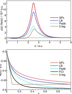
The resulting local slopes in the H2molecule with bond
length of 1.4 a.u. and 6.0 a.u. are plotted along the H–H bond in Figure 1, along with the densities from which they are calculated, at the FCI level of theory and in the uncontracted aug-cc-pCVTZ basis set.80 In both cases,
the local slope is greatest in magnitude at the nuclei, as has been seen previously in atoms.47 It can be seen that the magnitude of the local slope is significantly larger in
1 2 3 4 5
z / a.u. -0.4
-0.3 -0.2 -0.1 0
-ρ(z) / a.u.
0 2 4 6 8 10
z / a.u. -0.5
-0.4 -0.3 -0.2 -0.1 0
[image:5.612.322.563.51.327.2]-ρ(z) a.u.
FIG. 1. Plots comparing the values of−ρ(r) andw00(r), with
respect to the distance from the bond midpoint,z/ a.u., along the principal axis of the H2molecule with bond lengths of 1.4
a.u. (upper panel) and 6.0 a.u. (lower panel).
� � � � � �
-���� -���� -���� -���� ����
� �/����
Z=1
Z=2
Z=6
Z=10
FIG. 2. Plots ofw00(r) for the helium isoelectronic series, with
nuclear charges 1≤Z ≤ 10, and with radial distance from the nucleusr/ a.u. scaled by nuclear charge.
the stretched H2molecule, mirroring observations
previ-ously made of the global AC in the dissociating hydrogen molecule.51
[image:5.612.320.564.397.552.2]� � �� �� �� -����
-���� -���� -���� -���� -����
� �/���� Z=10 Z=8
Z=6
[image:6.612.53.299.49.203.2]Z=4
FIG. 3. Plots ofw00(r) for the beryllium isoelectronic series,
with nuclear charges 4 ≤Z ≤ 10, and with radial distance from the nucleusr / a.u. scaled by nuclear charge.
the uniform scaling condition,
lim γ→∞
Exc[ργ]
Ex[ργ]
= 1, with ργ(r) =γ3ρ(γr) (19)
which holds for non(near)degenerate KS systems.81 In Figure 2, it can be seen that the slope of the AC for the He series becomes less negative with increasing Z, tending to an asymptotic value as Z → ∞, consistent with the scaling relation of eq 19. However, the slope of the AC in the Be isoelectronic series becomes more negative with increasing Z, indicating that the scaling relation is not satisfied by this series.82
2. A functional approximation for the local slope
Whilst it is useful to numerically approximate the lo-cal slope for the purposes of evaluating lolo-cal interpolation schemes, such functionals would only be viable for main-stream use in DFT calculations if they can be described by simple functional forms.
In global models, the initial slope can be calculated directly from the occupied and virtual KS orbitals ac-cording to GL2 theory,
W00[ρ] = 2EcGL2[{φp, p}] =−1
2
X
abij
|hφiφj||φaφbi|2 a+b−i−j
−2X ia
|hφi|vˆxKS−ˆvxHF|φai|2
a−i ,
(20)
where the indicesi, janda, bpertain to occupied and vir-tual KS orbitals respectively, ˆvKS
x is the local KS
poten-tial and ˆvHF
x the non–local Hartree–Fock (HF) exchange
potential. The first term in eq 20 is analogous to the correlation energy given by MP2 theory, in whichφp and p are canonical HF orbitals and eigenvalues rather than
KS ones. The second term accounts for the difference between the KS and HF exchange potentials and has a form similar to a singles term in many–body perturba-tion theory. Previous studies of GL2 theory have found that the second term, although non–negligible, is small in magnitude relative to the MP2–like term evaluated with the KS orbitals.83 Therefore, it follows that an approx-imation to the GL2 correlation energy may be obtained by evaluating the MP2 correlation energy17with the KS
orbitals and eigenvalues,EGL2
c ≈EcMP2.
Given that an approximation to the global AC slope may be obtained from an MP2–like calculation, it follows that an approximation to the local AC slope may be ob-tained by deriving a local form of this expression. Whilst MP2 theory treats perturbations of the wavefunction, the analysis may be extended to energy densities in the gauge of the XC–hole by means of eq 10, as the substitution of eq 16 into eq 17 yields the following,
w00(r) = 1 2ρ(r)
Z P0 2(r,r0)
|r−r0| dr
0, (21)
where P20(r,r0) is the derivative of the pair–density at
λ= 0,
P20(r,r0) = ∂P2,λ(r,r
0)
∂λ
λ=0
. (22)
Notice that eq 21 ensures that w00(r) is in the gauge of the electrostatic potential of the xc hole. Given a non–interacting ground–state wavefunction Ψ(0), the
per-turbed wavefunction Ψλ for|λ|<<|Ψ(1)−Ψ(0)|2 can be appproximated by the series expansion
Ψλ=
X
n=0
λnΨ(n). (23)
If one assumes that Ψ(0) is non–degenerate and has the form of a single Slater determinant, the first–order cor-rection to the wavefunction is given by
Ψ(1)=X k
hΨ(0)k |Wˆ −VˆHF|Ψ(0)i
E0(0)−Ek(0)
Ψ(0)k . (24)
Restricting the space of Ψ(0)k to doubly–excited determi-nants reduces this expression to
Ψ(1)=−X
abij
hΨab
ij|Wˆ −VˆHF|Ψ(0)i
a+b−i−j
Ψabij. (25)
In MP2 theory, contributions to the correlation energy from singly–excited determinants are necessarily zero due to Brillouin’s theorem. However, this is not strictly true in GL2 theory as the singles term in eq 20 makes a small, but non–zero, contribution to the GL2 correlation energy.55As such, considering only double–excitations in
[image:6.612.95.276.567.648.2]Application of the Slater-Condon rules to eq 25 allows it to be re–written as
Ψ(1) =−1 4
X
abij
hij||abi
a+b−i−j
Ψabij, (26)
where the coefficient to Ψab
ij may be identified as an MP2 doubles–amplitudetab
ij,
tabij = hij||abi
a+b−i−j. (27) To obtain P0
2(r,r0), it is necessary to take the
deriva-tive of the pair–density corresponding to the perturbed wavefunction, Ψλ≈Ψ(0)+λΨ(1). Substituting this into eq 10 and rearranging the resulting expressions yields the following,
P20(r,r0) =N(N−1)X σ
Z ∂|Ψ
λ|2 ∂λ
λ=0
dr3..drN
=N(N−1)X σ
Z
|2Ψ(0)Ψ(1)|dr3..drN
= 2DΨ(0)
ˆ P2(r,r0)
Ψ
(1)E,
(28)
where we assume that Ψ(0) and Ψ(1) are real and
ˆ
P2(r,r0) = N(N−1)P
i6=j
δ(r−ri)δ(r−rj) is the pair– density operator. Substituting eq 26 into this expression gives,
P20(r,r0) =−X
abij
tabijhΨ(0)|Pˆ2(r,r0)|Ψabiji, (29)
which may then be resolved into the following orbital– explicit expression,
P20(r,r0) =−2X abij
tabij φi(r)φj(r0)φa(r)φb(r0)δσiσaδσjσb
−φi(r)φj(r0)φb(r)φa(r0)δσiσbδσjσa , (30) where δσiσa is the Kronecker’s delta over two spin func-tions: δσiσa =
R
σ∗i(ms)σa(ms)dms. Substituting eq 30 into eq 21 finally results in an expression for the local slope,
w00(r) =− 1 2ρ(r)
X
abij
tabijvabij(r), (31)
wherevabij(r) is theantisymmetrized orbital potential,
vabij(r) =φi(r)φa(r)
Z φ
j(r0)φb(r0)
|r−r0| dr 0δσ
iσaδσjσb
−φi(r)φb(r)
Z φj(r0)φa(r0) |r−r0| dr
0δσ
iσbδσjσa. (32) Multiplying the right–hand side of eq 31 by the density and integrating over all space, we recover twice the MP2
like expression. This is not an exact expression for the local slope, as the second term of eq 20 is not accounted for. However, the omitted term is generally small rela-tive to the MP2–like term, and vanishes entirely for two– electron systems, hence the expression for the local slope in eq 31 should, in principle, be a fair approximation of the exact local slope.
In future work we will implement and test eq 31 against the numerical results in section III A 1. The doubles am-plitudestab
ij are readily obtainable from standard quan-tum chemical packages, the potentialvabij(r) can also be readily calculated; however, it would likely be computa-tionally expensive to evaluate on a numerical grid. To reduce this cost a range of techniques, commonly used to accelerate the calculation of integrals in linear–scaling software packages, may be employed.26,84–86
We note that the behaviour of the local slopes pre-sented in Figures 1, 2 and 3 may be rationalized in a similar manner to that commonly discussed for global models in terms of eq 20. This is because of the key role of the doubles amplitudetab
ij in eq 31. The doubles amplitude has a dependence on the orbitals and orbital energies that is similar to that of the GL2 energy in eq 20. We see in Figure 1 that the local slope of the hydrogen molecule displays the minima at the nuclei. Equation 31, which is exact for two–electron systems, can be used to rationalize this observation. For closed shell two–electron systems with only one virtual orbital, eq 31 is simplified as follows:
w00(r) =−h11|22iφ1(r)φ2(r)
ρ(r)(2−1)
Z φ
1(r0)φ2(r0)
|r−r0| dr
0. (33)
Even if we used an orbital minimal basis for the evalu-ation of the expression given in eq 33 for the hydrogen molecule, we would see that the local slope displays the minima at the two nuclei for any bond length. While the appearance of the minima is being captured with the minimal basis, the same minimal basis model would in-correctly describe the slope at the midbond. For exam-ple, in the top panel of Figure 1 we see thatw00(r) is less than 0 at the midbond of H2 at R = 1.4. Within the
minimal basis, the local slope would be exactly 0 for any R, as the antibonding φ2(r) orbital which enters eq 33
has a node at the midbond.
We also see in Figure 2 that the correlation energy den-sity for the He isoelectronic series scales quickly towards an asymptotic constant asZincreases. Furthermore, the local slope decays smoothly with distance from the nu-cleus, reflecting the behaviour ofvabij(r). The behaviour for the Be isoelectronic series in Figure 3 is more com-plex. The KS HOMO-LUMO gap is known to increase87
asZincreases from 4 to 10, from which one would expect the correlation energy to become less negative according to the behaviour oftab
nu-merator oftabij and the spatial dependence ofvabij(r) due to the form of the KS orbitals are dominant in this re-gion, provided that eq 31 is sufficiently accurate for the Be isoelectronic series.
B. The SCE model and the strong interaction limit
In recent years, the exact strong-coupling limit of the AC has been intensively studied.29,33–37 This limit
re-veals a new structure for the XC functional: instead of the traditional ingredients of DFAs (local density, den-sity gradients, KS kinetic energy denden-sity, occupied and unoccupied KS orbitals) it is observed that certain inte-grals of the densityappear in this limit, encoding highly non-local information.33,35,38–40
Tests on model physical and chemical systems (elec-trons confined in dimensional geometries and low-density, ultracold dipolar systems, simple stretched bonds and anions) have shown35,37,39,40,88–90 that taking
into account this exact behaviour can pave the way for the solution of the strong correlation problem in DFT. However, the exact information encoded in the infinite coupling limit, described by the SCE functional, does not come for free: the SCE problem is ultra non-local, and, although sparse in principle, its non-linearity makes its exact evaluation for general three-dimensional geom-etry a complex task. A possible route to find suitable algorithms relies on the fact that constructing the exact SCE functional for a given density is equivalent to solv-ing an optimal transport (or mass transportation the-ory) problem with a cost function given by the Coulomb interaction.91,92 This equivalence has triggered interest from the applied mathematics community working on optimal transport problems, which has led to the sug-gestion of several algorithms,89,93–95 together with very
interesting exact results.96–98
So far, the SCE solution is known exactly for one-dimensional systems.41 For spherically symmetric
sys-tems, a conjectured solution33 that is very close to the exact one64 (and it is in many cases, but not always,98 exact) has been proposed and used to address interesting physical problems.90,99 Using algorithms and ideas from
optimal transport, the SCE problem for the hydrogen molecule along the dissociation curve has just recently been solved and both the global37,89 and local37 SCE quantities have been computed. A more practical way to proceed is to build approximations for the SCE functional inspired by its exact form, as it was done in the construc-tion of the already menconstruc-tioned NLR funcconstruc-tional.43,44
The SCE system complements the KS system.33,34,38
It corresponds to the wave function that minimizes the Hamiltonian of eq 1 when λ→ ∞. One can argue that the SCE system is a better starting point than the Kohn-Sham system for the description of very strongly corre-lated systems.37,39,40,89
The SCE functional is defined as29,33,35: WSCE[ρ] =hΨ
∞[ρ]|Wˆ|Ψ∞[ρ]i. (34)
The XC part Wxc,∞[ρ] can be easily extracted from WSCE[ρ], as W
xc,∞[ρ] = WSCE[ρ] −U[ρ]. The KS
SCE approximation, proposed in ref 35, uses the SCE functional to approximate the Hartree and exchange-correlation energy, and it is equivalent to settingWλ[ρ] =
W∞[ρ] for all λ. It has been shown that KS SCE yields
good energies for systems where correlation plays a dom-inant role, like electrons confined in low-density nanode-vices or extremely stretched bonds.37,39,40,89On the other
hand, KS SCE treats moderately and weakly correlated systems very poorly, giving energies that are unaccept-ably too low.37,88A less drastic approximation is to
con-struct aWλ[ρ] model, in such a way that itsλ→ ∞limit is given by the exact or approximate value ofW∞[ρ], as
done in the pioneering work of Seidl et. al.58,59
Anal-ogously, one can also model wλ(r), imposing that its λ → ∞ limit is given by w∞(r). This latter approach
is the main object of the following sections.
In the SCE limit, the electrons are infinitely or per-fectly correlated and their positions are given by an infi-nite superposition of classical configurations. The basic idea is that the electronic positions are all determined by a collective variabler, a feature that is captured by the so-called co-motion functions fi(r).33 If a reference electron is at r, then the position of all the other elec-trons in the system will be given byri =fi(r).33 Since
the electrons are perfectly correlated, the probability of finding the reference electron atrhas to be the same as the probability of finding theith electron atfi(r). There-fore, the co-motion functions have to satisfy the following differential equation:33
ρ(fi(r))dfi(r) =ρ(r)dr. (35) For more details on the co-motion functions, including their group properties, see Refs. 29,91,99 and 33.
In terms of the co-motion functions, the SCE func-tionalWSCE[ρ] is given by29
WSCE[ρ] =1
2
Z
drρ(r) N
X
i=2
1 |r−fi(r)|
. (36)
Despite the high nonlocality of the SCE functional, ev-ident from eq 35, we can easily compute its functional derivative from the following expression35,91
∇vSCE(r) =−
N
X
i=2
r−fi(r)
|r−fi(r)|3. (37) Equation 36 suggests the following energy density in the SCE limit:
w∞(r) =
1 2
N
X
i=2
1 |r−fi(r)|−
1
where vH(r) is the Hartree potential. This expression is
indeed in the gauge of the XC hole potential of eq 8, as proven in ref 29. Being derived from a wavefunction, thew∞(r) energy density decays like∼ −21|r|, similar to
the physical (λ = 1) and the exchange (λ = 0) energy densities of eq 16. Its functional derivative, eq (37), has also the correct asymptoticvxc∼ −|1r| behaviour.
To solve the SCE problem for spherically symmetric systems (the He and Be isoelectronic series considered in this paper) we have used the approach presented in ref 33, which is exact if N = 2. For atomic densities with N > 2 it could be either a very good approxima-tion for the true minimum of eq 34, or again, the exact result.64,98 For the H
2molecule we have used the results
of ref 37, where the SCE energy density has been com-puted by obtaining the co-motion function from the dual Kantorovich formulation91,100 of the SCE problem.
C. Local interpolation models
The local interpolation models tested in this work are largely simple translations of the well–established global interpolation models into a local form. This was done for the model of Seidl, Perdew and Levy (SPL),58 the
“sim-plified” model of Liu and Burke,61which will be referred
here as the LB model and the Pad´e[1/1] model.30,101
Each of the energy densities resulting from the three men-tioned models is constructed from three local parameters, a,bandc, which are defined in the gauge of the XC–hole. The functional forms of these three models are summa-rized in Table I.
In addition to these, we constructed a local form of the two–legged representation31 which, given some value of w1(r), takes the form
wλ(r) =
(
w0(r) +λw00(r), λ6xλ
w1(r), λ > xλ
(39a)
xλ=
w1(r)−w0(r)
w00(r) . (39b)
Whenever we used the two–legged representation to model the local AC in this work, we did it by in-corporating the interpolated w1(r) of the LB model:
w1(r) ≈ wLB1 (r). By doing the local interpolation this
way, we use the following three input quantities: w0(r),
w00(r) and w∞(r) and circumvent the direct utilization
of the full interacting energy density, w1(r). In each of
these four models, integration of wλ(r) with respect to coupling–constant gives the λ–averaged energy density
¯
wxc(r) which, if spatially integrated according to eq 7,
yields the XC–energyExc[ρ].
An important observation in the translation of global to local models is that, whilst the following global in-equalities are always satisfied,
W0[ρ]≥Exc[ρ]≥ W1[ρ]≥ W∞[ρ], (40)
their local counterparts do not necessarily satisfy these same inequalities. It has previously been observed for the Hooke’s atom series that, in the tail regions of the density, w∞(r) can be less negative than w1(r).29 In this work,
the crossing ofw∞(r) with ¯wxc(r),w1(r) and w0(r) has
only been observed in the tail regions of the density and is thought to be an artefact of the numerical instability that occurs where the density is very small.
IV. RESULTS
A. Helium isoelectronic series
Although the helium isoelectronic series is a set of only two–electron systems, it is a useful series to con-sider in evaluating the local interpolation models as most standard DFAs incorrectly characterize the hydride ion (H−), failing to predict its existence as a bound electronic system.66,102 Here, local interpolation models are
con-structed from energy densities acquired by the Lieb max-imisation at the FCI level, as described in section II D, in the range 0≤λ≤1 and atλ=∞by evaluating the SCE functional on the λ = 1 density, also at the FCI level of theory.
In Table II, the correlation energies given by local forms of the SPL, LB, two-legged representation (the column labelled “2–leg”) and Pad´e[1/1] models (the lat-ter paramelat-terized using the accurate values for w1(r),
in order to compare with models that, instead, use the λ→ ∞information) are given, along with that given by the global SPL model and the FCI correlation energy for comparison. This data shows that the local interpolation correlation energies are in close agreement with the FCI reference values; the mean absolute errors (MAE) of the local interpolation models are 2.0 mH, 1.5 mH, 0.5 mH and 0.1 mH, for the two-legged representation, SPL, LB and Pad´e[1/1] models, respectively.
[image:9.612.88.296.472.534.2]As would be expected, the local Pad´e[1/1] is the most accurate of the models, given that it is derived from the full interacting energy density. This data further suggests that the local LB model is marginally superior to the local SPL and the two-legged representation. However, comparing the global and local models shows a slightly lower error for the global model; the local SPL model has an MAE of 1.5 mH, compared to 1.3 mH for the global model.
Figure 4 compares the FCI ¯wc(r) with that of the local
LB and SPL models, for the helium atom. This reflects the numerical data in Table II, both being very close to the FCI energy density but with slightly lower error in the LB model.
B. Beryllium isoelectronic series
TABLE I. The mathematical forms of the local AC interpolation models (for the Pad´e[1/1] model,p >0,p∈R).
wλ(r) a(r) b(r) c(r) Refs.
SPL a+√ b
1+cλ w∞(r) w0(r)−w∞(r) −
2w00(r)
w0(r)−w∞(r) 33,58
LB a+b 1
(1+cλ)2 +√1+1cλ
w∞(r) (w0(r)−w∞(r))/2 − 4w
0 0(r)
5(w0(r)−w∞(r)) 61
Pad´e[1/1] a+ bλ
1+cλ w0(r) w
0
0(r)
−w0(r)+wp(r)−w00(r)
w0(r)−wp(r) 30,101
TABLE II. Reference and interpolatedEcvalues, in Hartree, for the He isoelectronic series.
Z FCI local SPL global SPL local LB Pad´e[1/1] local 2–leg
1 -0.0409 -0.0367 -0.0368 -0.0398 -0.0401 -0.0477
2 -0.0400 -0.0378 -0.0380 -0.0394 -0.0399 -0.0435
3 -0.0410 -0.0393 -0.0395 -0.0404 -0.0409 -0.0431
4 -0.0416 -0.0402 -0.0404 -0.0411 -0.0415 -0.0433
5 -0.0418 -0.0408 -0.0409 -0.0415 -0.0418 -0.0433
6 -0.0419 -0.0410 -0.0411 -0.0416 -0.0418 -0.0431
7 -0.0414 -0.0407 -0.0408 -0.0412 -0.0414 -0.0423
8 -0.0412 -0.0405 -0.0406 -0.0410 -0.0412 -0.0420
9 -0.0411 -0.0405 -0.0406 -0.0409 -0.0411 -0.0419
10 -0.0411 -0.0405 -0.0407 -0.0408 -0.0411 -0.0418
FIG. 4. Plots comparing the FCI, local LB and local SPL
λ–averaged correlation energy density in the helium atom.
those in the helium isoelectronic series, and its expla-nation involves the interplay of several effects. With increasing nuclear charge, the density becomes increas-ingly contracted, suggesting that the correlation energy should approach the high–density limit for very largeZ. However, this is accompanied by a changing KS HOMO– LUMO gap, here the energy difference between 2s and 2p orbitals, which increases from Z = 4 → 13 before decreasing with higherZ values.87
[image:10.612.223.563.224.508.2]Table III shows the reference and interpolatedEc re-sults for the Be isoelectronic series, with Z in the range
TABLE III. Reference and interpolatedEcvalues, in Hartree, for the Be isoelectronic series.
Z CCSD local SPL global SPL local LB Pad´e[1/1] local 2–leg
4 -0.0920 -0.0876 -0.1049 -0.0925 -0.0911 -0.1046
5 -0.1089 -0.1041 -0.1250 -0.1100 -0.1076 -0.1246
6 -0.1244 -0.1202 -0.1455 -0.1271 -0.1229 -0.1444
7 -0.1389 -0.1363 -0.1668 -0.1443 -0.1373 -0.1645
8 -0.1534 -0.1532 -0.1898 -0.1626 -0.1517 -0.1859
9 -0.1683 -0.1717 -0.2157 -0.1826 -0.1666 -0.2098
[image:10.612.52.317.229.540.2]10 -0.1833 -0.1920 -0.2447 -0.2046 -0.1817 -0.2361
FIG. 5. Plots comparing the CCSD, local LB and local SPL
λ–averaged correlation energy density in the beryllium atom.
4−10. The wave function forλvalues between 0 and 1 has been computed in the same way as for the He isoelec-tronic series, however at the CCSD level of theory rather than FCI. As for the helium series, the local Pad´e[1/1] that uses w1(r) is the most accurate of the local
inter-polation models. However, in contrast to the findings for He isoelectronic series, the local interpolation mod-els are much more accurate than the global modmod-els. For example, in the case of F5+ the global SPL model has
Figure 5 shows theλ–averaged correlation energy den-sities for the beryllium atom. The shape of ¯wc(r)
re-flects the shell structure of the Be atom.47,82 The local
SPL and LB interpolation models appear to qualitatively capture the shell structure of ¯wc(r), however in some
re-gions it overestimates the reference value whilst in other regions the converse is the case. The error cancellation that results from this is the most likely explanation for the superior accuracy of the local models in comparison to the global models.
C. Hydrogen molecule
Despite the development of DFT into the most widely– applied electronic structure method, and the wealth of XC–DFAs that have been developed, there are some sys-tems for which no combination of DFAs provide an ac-curate description. A well–known example of such a sys-tem is the dissociating H2molecule.42,103Standard DFAs
become increasingly inaccurate with greater H–H bond length, reflecting a fundamental flaw of DFAs in their inability to properly treat strong correlation.
It has been seen previously37,89that KS SCE correctly
predicts the dissociation of H2 in a spin–restricted
for-malism, however at equilibrium geometry the energies it predicts are extremely low and the bond lengths pre-dicted are overly short. The overall accuracy of KS-SCE for H2dissociation can be substantially improved by the
addition of nonlocal corrections.37
Figure 6 shows the dissociation curves for H2 given
by the local interpolation models, along with those given by HF, FCI and the PBE functional5 for comparison.
The computational details are the same as those of the He isoelectronic series, and the PBE, HF and FCI curves have been obtained from theDaltonquantum chemistry package78all within the uncontracted aug-cc-pCVTZ ba-sis set.80The SCE energy density has been computed by using the dual Kantorovich method.37
It can be seen in Figure 6 that all of the interpolation models correctly predict the dissociation of H2, which
fol-lows from their inclusion of w∞(r). In global AC
mod-els, at infinite separation the initial slope diverges as a result of the vanishing HOMO–LUMO gap, and the SPL and LB models reduce toW∞[ρ], yielding the exact
en-ergies. However, the dissociation curves produced by the local models approach the FCI curve slowly, resulting in an unphysical ‘bump’–like feature. This is a well–known failing of DFT, having been observed with other func-tionals, such as the random–phase approximation103and even the global Pad´e[1/1] model withW1[ρ].65 It can be
seen in Figure 6 that this is not remedied by the local interpolation approach, as the curve obtained by the lo-cal Pad´e[1/1] also exhibits this unphysical bump, as does that given by the local SPL model and, to a lesser extent, the local LB model.
To analyse why the intermediate region is less accu-rately described by the local interpolation methods than
the equilibrium and stretched region, we show in Fig-ure 8 the correlation component of the local AC at one of the nuclei of the hydrogen molecule at different bond lengths: R= 1.4 a.u. (at equilibrium),R= 5.0 a.u. (the intermediate region) andR= 13.0 a.u. (stretched bond). The structure of the three local AC curves at one of the nuclei is very similar to the structure of the correspond-ing global AC curves.50From the given figure we see that
at equilibrium the local AC is almost linear, so we can expect that even a single line segment approximation to the local AC:wλ(r)≈w0(r) +w00(r) would properly
cap-ture the shape of the given local AC curve. The local AC curve at the nuclei of the stretched H2 exhibits the
characteristic ‘L-shape’, which was also observed in the case of the corresponding global AC curve.50 We would
expect that the two-legged representation would capture the given local AC very well, but even a single line seg-ment approximation: wλ(r)≈w∞(r), this time coming
from the strong coupling limit, would be highly accu-rate for the stretched H2.37 In contrast to the local AC
curves of the stretched and H2 at equilibrium, the
cur-vature of the local AC curve at the intermediate bond length is highly pronounced. The shapes of the local AC curves at the nuclei mirror the difference in correla-tion regimes present in the hydrogen molecule at differ-ent bond lengths. While in the H2at equilibrium and at
very stretched bond length, correlation is almost purely dynamical and almost purely static, respectively, in the intermediate dissociation region there is a subtle inter-play between the dynamical and static correlation.
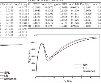
In the intermediate region of the dissociation curve, where the unphysical bump is present, the local two-legged representation model is more accurate than the local Pad´e[1/1] which we always use here with w1(r).
This may be understood by comparing the exact local AC data with the interpolated quantities. The top panel of Figure 8 shows the difference between ¯wFCI(r) and
that of each of the local interpolation models, along the H–H bond at the 5.0 a.u. geometry, as a function of the distance from the bond midpointz. This difference δw(r) = ¯wFCI(r)−w¯model(r), is multiplied by the
den-sity to represent an energy per volume element. It shows that the local SPL energy density is the one that most overestimates the ¯w(r). The error is smaller for the LB model and even more so for the local Pad´e[1/1] model. The error is smallest in the two–legged model, obtained using the w1(r) of the local LB. Furthermore, there is
the error cancellation in the two–legged model, as there are regions where the ¯w(r) of this model underestimates
¯ wFCI(r).
It can also be seen that the curves shown in the top panel of Figure 8 have a maximum at the nucleus (z = 2.5). Focusing on this region, it appears that the FCI curve meets that of the Pad´e[1/1] atλ= 1, and that the two–legged representation curve meets that of the LB model also atλ= 1. This follows from the construction of the Pad´e[1/1] and two–legged curves fromw1FCI(r) and wLB
2 4 6 8 10 12
R / a.u.
-1.1 -1 -0.9 -0.8
E(R
)
/
a
.u
.
[image:12.612.57.561.54.338.2]HF
PBE
SPL
LB
Padé
2-leg
FCI
FIG. 6. Potential energy curves for the H2 molecule with internuclear distanceR / a.u., which are obtained using the local
interpolation methods: SPL, Liu-Burke, two-legged representation combined with the Liu-Burke model, Pad´e[1/1] withw1(r).
Restricted HF, PBE and FCI curves are also shown for comparison.
0 0.2 0.4 0.6 0.8 1
λ -0.2
-0.15 -0.1 -0.05 0
wc
(
λ
) / a.u. R=1.4
R=5.0 R=13.0
FIG. 7. The FCI local correlation AC curves at one of the nuclei of H2for different bond lengths.
two-legged model, lie above the FCI curve. In the case of the two–legged interpolation model, the first line segment is below the FCI curve, as a result of eq 39a and the convexity of the given local AC curve. The second line segment that starts atxλ∼0.1 is given bywLB1 (r), and
lies above the FCI curve. The resulting error cancellation makes it clear why the two–legged representation appears
more accurate than the other models.
V. CONCLUSION AND PERSPECTIVES
In this work we have studied local interpolations along the adiabatic connection for the He and Be isoelectronic series and the hydrogen molecule, by using accurate input local quantities computed in the gauge of the electrostatic potential of the XC hole, and comparing the results with nearly exact energy densities defined in the same way. In order to obtain approximations to the local AC over the physical regime (0≤ λ ≤1), we constructed inter-polation models between the weak and strong coupling limits of DFT. The weak coupling energy densities were obtained using the Lieb variation principle, whilst the strong coupling limit energy densities were obtained us-ing the strictly-correlated electrons (SCE) approach. The inclusion of the SCE information in density functional ap-proximations helps to ensure their ability to capture the strong correlation effects.
[image:12.612.55.305.408.576.2]avoid-0 1 2 3 4 5 6 z / a.u.
0 2 4 6 8 10 12
ρ
(z)
δ
w(z) /
10
-3 a.u.
SPL LB Padé 2-leg
0 0.2 0.4 0.6 0.8 1 λ
-0.5 -0.45 -0.4 -0.35 -0.3
w
(
λ
)
/
a
.u
. SPL
[image:13.612.57.310.53.384.2]LB Padé FCI 2-leg
FIG. 8. Plots of the difference between FCI and interpolated
λ–averaged energy densities, δw(z) = ¯wFCI(z)−w¯model(z),
with respect to the distance from the bond midpoint,z/ a.u. (upper panel), and the local AC curves at one of the nuclei of the FCI and local interpolation models (lower panel), both in H2 with a 5.0 a.u. bond length.
ing to mimic strong correlation with symmetry breaking, some care must be taken when discussing size consis-tency. In fact, strictly speaking, in a restricted framework the energy densities of the second-order perturbation the-ory and exact exchange are not intensive quantities in the presence of near degeneracy,67,68 which is the main chal-lenge of capturing strong correlation within DFT.104–106 In future work we will test different approximations for the SCE energy densities and the local slope. The development of algorithms for solution of the SCE prob-lem is a very active research field. In spite of the recent improvements, we still lack an algorithm that will solve the SCE problem for general 3D molecular geometries at low computational cost. However, a good candidate to approximate the SCE energy density in the gauge of the XC hole potential is the nonlocal radius functional (NLR),43 which has been already implemented and used in ref 44.
In addition to numerically exploring the local AC we have also reported the local weak-coupling slope of the
adiabatic connection and derived an approximate expres-sion for it in terms of occupied and unoccupied orbitals. This quantity is very important to signal the amount of correlation at each point of space. In our future work we will implement this expression and test it against the results reported here.
ACKNOWLEDGEMENTS
We are very grateful to Derk Kooi and Andr´e Mirtschink for a critical reading of the manuscript and in-sightful suggestions to improve it. We acknowledge finan-cial support from the European Research Council under H2020/ERC Consolidator Grant corr-DFT (Grant No. 648932) and the Netherlands Organization for Scientific Research (NWO) through an ECHO grant (717.013.004). A. M. T. is grateful for support from the Royal Society University Research Fellowship scheme. A. M. T and T. J. P. I. are grateful for support from the Engineer-ing and Physical Sciences Research Council (EPSRC), (Grant No. EP/M029131/1). We are grateful for ac-cess to the University of Nottingham High Performance Computing Facility.
1W. Kohn and L. J. Sham, Phys. Rev.140, A 1133 (1965).
2C. Lee, W. Yang, and R. G. Parr, Phys. Rev. B37, 785 (1988).
3A. D. Becke, Phys. Rev. A38, 3098 (1988).
4J. P. Perdew, J. A. Chevary, S. H. Vosko, K. A. Jackson, M. R.
Pederson, D. J. Singh, and C. Fiolhais, Phys. Rev. B46, 6671
(1992).
5J. P. Perdew, K. Burke, and M. Ernzerhof, Phys. Rev. Lett.
77, 3865 (1996).
6Y. Zhao and D. G. Truhlar, J. Chem. Phys.128, 184109 (2008).
7J. Tao, J. P. Perdew, V. N. Staroverov, and G. E. Scuseria,
Phys. Rev. Lett.91, 146401 (2003).
8R. Peverati and D. G. Truhlar, Phil. Trans. R. Soc. A 372,
20120476 (2014).
9J. Sun, A. Ruzsinszky, and J. P. Perdew, Phys. Rev. Lett.115,
036402 (2015).
10A. D. Becke, J. Chem. Phys.98, 5648 (1993).
11J. P. Perdew, M. Ernzerhof, and K. Burke, J. Chem. Phys.105,
9982 (1996).
12Y. Zhao, N. E. Schultz, and D. G. Truhlar, J. Chem. Theory
Comput.2, 364 (2006).
13J. P. Perdew and A. Zunger, Phys. Rev. B23, 5048 (1981).
14O. A. Vydrov and G. E. Scuseria, J. Chem. Phys.121, 8187
(2004).
15O. A. Vydrov and G. E. Scuseria, J. Chem. Phys.122, 184107
(2005).
16S. K¨ummel and L. Kronik, Rev. Mod. Phys.80, 3 (2008).
17S. Grimme, J. Chem. Phys.124, 034108 (2006).
18L. Goerigk and S. Grimme, J. Chem. Theory Comput.7, 291
(2010).
19K. Sharkas, J. Toulouse, and A. Savin, J. Chem. Phys. 134,
064113 (2011).
20F. Furche, Phys. Rev. B64, 195120 (2001).
21A. Hesselmann and A. G¨orling, Mol. Phys.108, 359 (2010).
22J. G. ´Angy´an, R.-F. Liu, J. Toulouse, and G. Jansen, J. Chem.
Theory Comput.7, 3116 (2011).
23J. Jaramillo, G. E. Scuseria, and M. Ernzerhof, J. Chem. Phys.
118, 1068 (2003).
24A. V. Arbuznikov and M. Kaupp, Chem. Phys. Lett.440, 160
25A. V. Arbuznikov and M. Kaupp, J. Chem. Phys.128, 214107 (2008).
26H. Bahmann and M. Kaupp, J. Chem. Theory Comput. 11,
1540 (2015).
27J. Harris, Phys. Rev. A29, 1648 (1984).
28D. C. Langreth and J. P. Perdew, Solid State Commun.17, 1425
(1975).
29A. Mirtschink, M. Seidl, and P. Gori-Giorgi, J. Chem. Theory
Comput.8, 3097 (2012).
30M. Ernzerhof, Chem. Phys. Lett.263, 499 (1996).
31K. Burke, M. Ernzerhof, and J. P. Perdew, Chem. Phys. Lett.
265, 115 (1997).
32P. Mori-Sanchez, A. J. Cohen, and W. T. Yang, J. Chem. Phys.
124, 091102 (2006).
33M. Seidl, P. Gori-Giorgi, and A. Savin, Phys. Rev. A75, 042511
(2007).
34P. Gori-Giorgi, G. Vignale, and M. Seidl, J. Chem. Theory
Comput.5, 743 (2009).
35F. Malet and P. Gori-Giorgi, Phys. Rev. Lett. 109, 246402
(2012).
36A. Mirtschink, M. Seidl, and P. Gori-Giorgi, Phys. Rev. Lett.
111, 126402 (2013).
37S. Vuckovic, L. O. Wagner, A. Mirtschink, and P. Gori-Giorgi,
J. Chem. Theory Comput.11, 3153 (2015).
38M. Seidl, Phys. Rev. A60, 4387 (1999).
39F. Malet, A. Mirtschink, J. C. Cremon, S. M. Reimann, and
P. Gori-Giorgi, Phys. Rev. B87, 115146 (2013).
40C. B. Mendl, F. Malet, and P. Gori-Giorgi, Phys. Rev. B89,
125106 (2014).
41M. Colombo, L. De Pascale, and S. Di Marino, Can. J. Math.
67, 350 (2015).
42S. Vuckovic, L. O. Wagner, A. Mirtschink, and P. Gori-Giorgi,
J. Chem. Theory Comput.11, 3153 (2015).
43L. O. Wagner and P. Gori-Giorgi, Phys. Rev. A 90, 052512
(2014).
44Y. Zhou, H. Bahmann, and M. Ernzerhof, J. Chem. Phys.143,
124103 (2015).
45A. D. Becke, J. Chem. Phys.138, 074109 (2013).
46J. Kong and E. Proynov, J. Chem. Theory Comput. 12, 133
(2015).
47T. J. Irons and A. M. Teale, Mol. Phys. , DOI:
10.1080/00268976.2015.1096424 (2015).
48E. H. Lieb, Int. J. Quantum. Chem.24, 24 (1983).
49Q. Wu and W. Yang, J. Chem. Phys.118, 2498 (2003).
50A. M. Teale, S. Coriani, and T. Helgaker, J. Chem. Phys.130,
104111 (2009).
51A. M. Teale, S. Coriani, and T. Helgaker, J. Chem. Phys.132,
164115 (2010).
52A. M. Teale, S. Coriani, and T. Helgaker, J. Chem. Phys.133,
164112 (2010).
53J. Harris and R. Jones, J. Phys. F4, 1170 (1974).
54O. Gunnarsson and B. I. Lundqvist, Phys. Rev. B 13, 4274
(1976).
55A. G¨orling and M. Levy, Phys. Rev. B47, 13105 (1993).
56A. G¨orling and M. Levy, Phys. Rev. A50, 196 (1994).
57M. Levy, Phys. Rev. A43, 4637 (1991).
58M. Seidl, J. P. Perdew, and M. Levy, Phys. Rev. A 59, 51
(1999).
59M. Seidl, J. P. Perdew, and S. Kurth, Phys. Rev. Lett.84, 5070
(2000).
60A. J. Cohen, P. Mori-S´anchez, and W. Yang, J. Chem. Phys.
127, 034101 (2007).
61Z. F. Liu and K. Burke, Phys. Rev. A79, 064503 (2009).
62A. M. Teale, S. Coriani, and T. Helgaker, J. Chem. Phys.132,
164115 (2010).
63C. M¨oller and M. S. Plesset, Phys. Rev.46, 618 (1934).
64S. Di Marino, A. Gerolin, L. Nenna, M. Seidl, and P.
Gori-Giorgi, “in preparation,”.
65M. J. G. Peach, A. M. Teale, and D. J. Tozer, J. Chem. Phys.
126, 244104 (2007).
66M. J. G. Peach, A. M. Miller, A. M. Teale, and D. J. Tozer, J.
Chem. Phys.129, 064105 (2008).
67P. Gori-Giorgi and A. Savin, J. Phys.: Conf. Ser.117, 012017
(2008).
68A. Savin, Chem. Phys.356, 91 (2009).
69K. Burke, F. G. Cruz, and K.-C. Lam, J. Chem. Phys. 109,
8161 (1998).
70F. G. Cruz, K.-C. Lam, and K. Burke, J. Phys. Chem. A102,
4911 (1998).
71J. Tao, V. N. Staroverov, G. E. Scuseria, and J. P. Perdew,
Phys. Rev. A77, 012509 (2008).
72K. Burke, F. G. Cruz, and K.-C. Lam, J. Chem. Phys. 109,
8161 (1998).
73R. Armiento and A. E. Mattsson, Phys. Rev. B66(2002).
74J. C. Slater, Phys. Rev.81, 385 (1951).
75B. G. Janesko, A. V. Krukau, and G. E. Scuseria, J. Chem.
Phys.129, 124110 (2008).
76E. Fermi and E. Amaldi, R. Accad. d’Italia. Memorie 6, 119
(1934).
77T. Helgaker and P. Jørgensen, Theor. Chim. Acta 75, 111
(1989).
78K. Aidas, C. Angeli, K. L. Bak, V. Bakken, R. Bast, L.
Bo-man, O. Christiansen, R. Cimiraglia, S. Coriani, P. Dahle, E. K.
Dalskov, U. Ekstr¨om, T. Enevoldsen, J. J. Eriksen, P.
Ettenhu-ber, B. Fern´andez, L. Ferrighi, H. Fliegl, L. Frediani, K. Hald,
A. Halkier, C. H¨attig, H. Heiberg, T. Helgaker, A. C.
Hen-num, H. Hettema, E. Hjertenaes, S. Høst, I.-M. Høyvik, M. F. Iozzi, B. Jans´ık, H. J. A. Jensen, D. Jonsson, P. Jørgensen, J. Kauczor, S. Kirpekar, T. Kjaergaard, W. Klopper, S. Knecht, R. Kobayashi, H. Koch, J. Kongsted, A. Krapp, K. Kristensen, A. Ligabue, O. B. Lutnaes, J. I. Melo, K. V. Mikkelsen, R. H. Myhre, C. Neiss, C. B. Nielsen, P. Norman, J. Olsen, J. M. H. Olsen, A. Osted, M. J. Packer, F. Pawlowski, T. B. Pedersen, P. F. Provasi, S. Reine, Z. Rinkevicius, T. A. Ruden, K. Ruud,
V. V. Rybkin, P. Sa lek, C. C. M. Samson, A. S. de Mer´as,
T. Saue, S. P. A. Sauer, B. Schimmelpfennig, K. Sneskov, A. H. Steindal, K. O. Sylvester-Hvid, P. R. Taylor, A. M. Teale, E. I. Tellgren, D. P. Tew, A. J. Thorvaldsen, L. Thøgersen, O.
Vah-tras, M. A. Watson, D. J. D. Wilson, M. Ziolkowski, and
H. ˚Agren, Wiley Interdiscip. Rev.: Comput. Mol. Sci. 4, 269
(2014).
79G. D. Purvis and R. J. Bartlett, J. Chem. Phys.76, 1910 (1982).
80T. H. Dunning, J. Chem. Phys.90, 1007 (1989).
81J. P. Perdew, V. N. Staroverov, J. Tao, and G. E. Scuseria,
Phys. Rev. A78, 052513 (2008).
82F. Colonna and A. Savin, J. Chem. Phys.110, 2828 (1999).
83J. Toulouse, K. Sharkas, E. Br´emond, and C. Adamo, J. Chem.
Phys.135, 101102 (2011).
84H.-J. Werner, F. R. Manby, and P. J. Knowles, J. Chem. Phys.
118, 8149 (2003).
85S. Reine, E. Tellgren, A. Krapp, T. Kjærgaard, T. Helgaker,
B. Jansik, S. Hoøst, and P. Salek, J. Chem. Phys.129, 104101
(2008).
86V. D. Dom´ınguez-Soria, G. Geudtner, J. L. Morales,
P. Calaminici, and A. M. K¨oster, J. Chem. Phys.131, 124102
(2009).
87A. Savin, F. Colonna, and R. Pollet, Int. J. Quantum. Chem.
93, 166 (2003).
88F. Malet, A. Mirtschink, K. Giesbertz, L. Wagner, and P.
Gori-Giorgi, Phys. Chem. Chem. Phys.16, 14551 (2014).
89H. Chen, G. Friesecke, and C. B. Mendl, J. Chem. Theory
Comput10, 4360 (2014).
90F. Malet, A. Mirtschink, C. B. Mendl, J. Bjerlin, E. O.
Karabu-lut, S. M. Reimann, and P. Gori-Giorgi, Phys. Rev. Lett.115,
033006 (2015).
91G. Buttazzo, L. De Pascale, and P. Gori-Giorgi, Phys. Rev. A
85, 062502 (2012).
92C. Cotar, G. Friesecke, and C. Kl¨uppelberg, Comm. Pure Appl.
Math.66, 548 (2013).
94J.-D. Benamou, G. Carlier, M. Cuturi, L. Nenna, and G. Peyr´e,
SIAM J. on Sci. Comput.37, A1111 (2015).
95J.-D. Benamou, G. Carlier, and L. Nenna, arXiv preprint
arXiv:1505.01136 (2015).
96M. Colombo, L. De Pascale, and S. Di Marino, Canad. J. Math
67, 350 (2015).
97S. Di Marino, A. Gerolin, and L. Nenna, arXiv preprint
arXiv:1506.04565 (2015).
98M. Colombo and F. Stra, arXiv preprint arXiv:1507.08522
(2015).
99C. B. Mendl, F. Malet, and P. Gori-Giorgi, Phys. Rev. B89,
125106 (2014).
100L. De Pascale, arXiv preprint arXiv:1503.07063 (2015).
101P. Mori-S´anchez, A. J. Cohen, and W. Yang, J. Chem. Phys.
125, 201102 (2006).
102A. Mirtschink, C. J. Umrigar, J. D. Morgan, and P. Gori-Giorgi,
J. Chem. Phys.140, 18A532 (2014).
103M. Fuchs, Y. M. Niquet, X. Gonze, and K. Burke, J. Chem.
Phys.122, 094116 (2005).
104A. Savin, in Recent Developments of Modern Density
Func-tional Theory, edited by J. M. Seminario (Elsevier, Amsterdam, 1996) pp. 327–357.
105A. J. Cohen, P. Mori-Sanchez, and W. Yang, Science321, 792
(2008).
106P. Mori-Sanchez, A. J. Cohen, and W. Yang, Phys. Rev. Lett.