APPLICATIONS OF LIE METHODS TO COMPUTATIONS WITH POLYCYCLIC GROUPS
Björn Assmann
A Thesis Submitted for the Degree of PhD at the
University of St. Andrews
2007
Full metadata for this item is available in the St Andrews Digital Research Repository
at:
https://research-repository.st-andrews.ac.uk/
Please use this identifier to cite or link to this item: http://hdl.handle.net/10023/435
Applications of Lie methods
to computations with polycyclic groups
A thesis to be submitted to the
UNIVERSITY OF ST ANDREWS
for the degree of
DOCTOR OF PHILOSOPHY
by
Bj¨orn Assmann
School of Computer Science University of St Andrews
I, Bj¨orn Assmann, hereby certify that this thesis, which is approximately 31000 words in length, has been written by me, that it is the record of work carried out by me, and that it has not been submitted in any previous application for a higher degree.
date signature of candidate
I was admitted as a research student in October 2004 and as a candidate for the degree of Doctor of Philosophy in October 2004; the higher study for which this is a record was carried out in the University of St Andrews between 2004 and 2007.
date signature of candidate
I, Stephen Linton, hereby certify that the candidate has fulfilled the condi-tions of the Resolution and Regulacondi-tions appropriate for the degree of Doctor of Philosophy in the University of St Andrews and that the candidate is qualified to submit this thesis in application for that degree.
date signature of supervisor
In submitting this thesis to the University of St. Andrews I understand that I am giving permission for it to be made available for use in accordance with the regulations of the University Library for the time being in force, subject to any copyright vested in the work not being affected thereby. I also understand that the title and abstract will be published, and that a copy of the work may be made and supplied to any bona fide library or research worker.
Abstract
In this thesis we demonstrate the algorithmic usefulness of the so-called Mal’cev correspondence for computations with infinite polycyclic groups. This correspondence betweenQ-powered nilpotent groups and rational nilpo-tent Lie algebras was discovered by Anatoly Mal’cev in 1951.
We show how the Mal’cev correspondence can be realized on a computer. We explore two possibilities for this purpose and compare them: the first one uses matrix embeddings and the second the Baker–Campbell–Hausdorff formula.
Then, we describe a new collection algorithm for polycyclically presented groups, which we call Mal’cev collection. Algorithms for collection lie at the heart of most methods dealing with polycyclically presented groups. The current state of the art is “collection from the left” as recently studied by Gebhardt, Leedham-Green/Soicher and Vaughan-Lee. Mal’cev collection is in some cases dramatically faster than collection from the left, while using less memory.
Further, we explore how the Mal’cev correspondence can be used to de-scribe symbolically the collection process in polycyclically presented groups. In particular, we describe an algorithm that computes the collection func-tions for splittable polycyclic groups. This algorithm is based on work by du Sautoy. We apply it to the computation of pro-p-completions of polycyclic groups.
Finally we describe a practical algorithm for testing polycyclicity of finitely generated rational matrix groups. Previously, not only did no such method exist but it was not clear whether this question was decidable at all.
Acknowledgement
I would like to thank my advisor Stephen Linton for our many inspiring discussions during my time at the University of St Andrews. In particular, I am grateful for his open-minded approach to our mathematical meetings where anything could be brought on the table. Although my work benefitted tremendously from our conversations, they are most memorable because they were genuinely enjoyable.
I would like to thank my second advisor Martyn Quick for his competent advice on infinite group theory and for carefully reading the first draft of this thesis.
Also, I am grateful to Bettina Eick for introducing me to the area of computational group theory, which became a very enjoyable mathematical playground for the years to follow.
Many thanks go to my office mate Peter Nightingale for his patient an-swers to my questions related to the English language and for being an ex-cellent riddle partner.
I gratefully acknowledge the financial support of the Gottlieb Daimler-und Karl Benz-Stiftung and the UK Engineering and Physical Science Re-search Council.
Contents
1 Introduction 11
2 Polycyclic groups 14
2.1 Preliminaries . . . 14
2.1.1 Poly-P groups . . . 16
2.1.2 Soluble groups . . . 16
2.1.3 Nilpotent groups . . . 17
2.2 Polycyclic sequences . . . 18
2.3 Polycyclic presentations . . . 19
2.4 Nilpotency, polycyclicity and solubility . . . 21
2.5 Structure of infinite polycyclic groups . . . 24
3 Mal’cev correspondence 25 3.1 Preliminaries . . . 25
3.2 Matrix correspondence . . . 27
3.3 Abstract correspondence . . . 31
4 Computing the correspondence 36 4.1 Via matrix embeddings . . . 36
4.2 Via the Baker–Campbell–Hausdorff formula . . . 38
4.3 Symbolic Log and Exp . . . 40
4.4 Runtimes and comparison . . . 41
5 Mal’cev collection 44 5.1 Classical collection . . . 44
5.2 Collection using the Mal’cev correspondence . . . 46
5.2.1 Choosing the polycyclic sequence G . . . 46
5.2.2 Mal’cev collection in H =CN . . . 47
5.2.3 Inversion in H =CN . . . 48
5.2.4 Powering in H =CN . . . 48
5.2.5 Mal’cev collection in G . . . 49
5.2.6 Inversion in G . . . 50
5.3 Computations with powers of automorphisms ofT-groups . . 50
5.4 Computations with consecutive powers of automorphisms of T-groups . . . 51
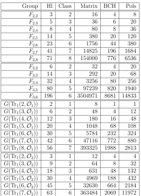
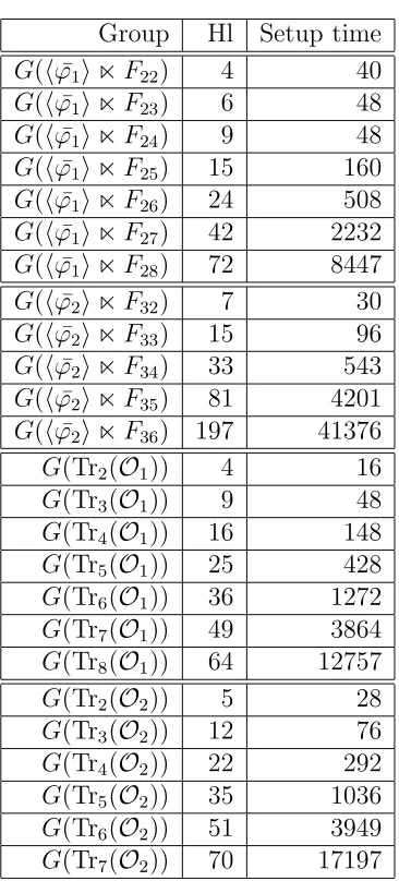
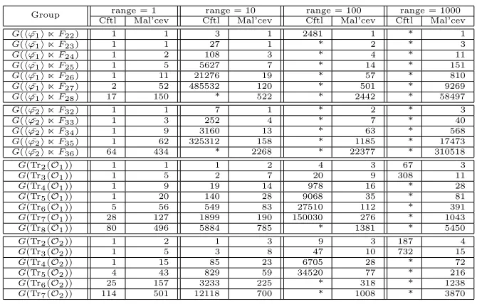
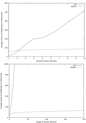
5.5 Implementation and runtimes . . . 51
5.5.1 Example groups . . . 51
5.5.2 Runtimes setup . . . 52
5.5.3 Mal’cev collection versus collection from the left . . . . 53
5.5.4 Concluding remarks . . . 57
6 Symbolic collection 58 6.1 Jordan decomposition . . . 59
6.2 Splittable polycyclic groups . . . 59
6.3 Computing collection functions . . . 61
6.3.1 The action of C onN . . . 61
6.3.2 Converting tails . . . 64
6.3.3 The algorithm . . . 65
6.4 Applications . . . 66
6.4.1 Collection . . . 67
6.4.2 pro-p-completions . . . 67
7 Alternatives beyond the Tits alternative 70 7.1 Deciding the Tits’ alternative . . . 71
7.1.1 Computing a semisimple series . . . 71
7.1.2 The p-congruence subgroup . . . 72
7.1.3 Testing (virtual) solvability . . . 73
7.1.4 Comparing classes of groups . . . 73
7.2 The Mal’cev correspondence and finite generation . . . 73
7.3 Checking conjugacy into GL(d,Z) . . . 75
7.4 Testing polycyclicity . . . 77
7.5 Testing virtual polycyclicity . . . 80
7.6 Testing nilpotency . . . 81
7.7 Testing virtual nilpotency . . . 84
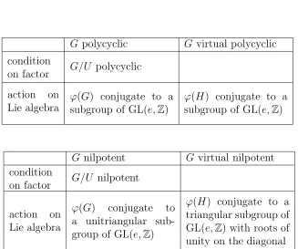
7.8 Summary . . . 85
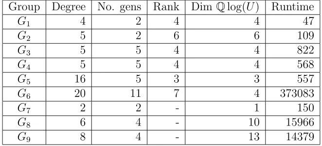
7.9 Implementation and examples . . . 87
7.9.1 Runtimes . . . 87
Chapter 1
Introduction
A group is the algebraic concept to describe symmetry. As a consequence, the theory of groups can be applied to various areas of science, for example ge-ometry, number theory, crystallography, quantum mechanics and constraint programming.
Because of its generality, the definition of a group allows very complicated structures. Thus, it is natural to apply a well-known approach from other sciences to the study of groups. Namely given a group G, decompose it into smaller more understandable pieces, study those, and finally study their interaction to reveal the structure of G.
The smallest pieces in group theory are called simple groups. One of the biggest algebraic projects of the last century was the classification of the finite simple groups. Its aim was the creation of a table that contains all finite simple groups up to isomorphism.
The theory of polycyclic groups aims in the opposite direction. It does not try to classify the atoms of group theory but asks: What can a group look like that is made out of easy pieces namely cyclic groups? Given the re-strictiveness of this question it is rather surprising that the class of polycyclic groups has a rich theory with interesting links to other areas, in particular number theory. It shows that the mechanism for building groups out of smaller ones, essentially the interaction between factor groups and normal subgroups, is rather complex.
Historically polycyclic groups were considered right from the start of group theory. Evariste Galois showed in the first half of the nineteenth century that a rational polynomial is soluble by radicals if and only if the symmetry group of its solutions is polycyclic. The foundations of the struc-tural explorations of polycyclic groups were laid roughly 100 year later by Kurt Hirsch, Phillip Hall, Reinhold Baer and Anatoly Mal’cev amongst oth-ers.
12 Chapter 1. Introduction
More recently the class of polycyclic groups has also been shown to be very fruitful for computational investigations, see for example [17, 39]. Polycyclic groups can be efficiently represented on a computer by means of a special kind of finite presentation, which is called a polycyclic presentation. If a group is given with respect to a polycyclic presentation, then various properties of the group can explored algorithmically. For example it is possible to test membership in subgroups, to compute the normal closure of subgroups and to determine the derived series.
The aim of this thesis is to show how Lie methods can be applied to the algorithmic investigation of polycyclic groups. The connection between groups and Lie rings, respectively Lie algebras, is a well-known and mathe-matically very useful concept. For example, a typical way to solve a problem in a Lie group is to transfer the problem to the Lie algebra of the group, study it there with the help of tools from linear algebra and transfer the result back into the Lie group.
Mechanisms of this kind have already been shown to be useful for the ex-ploration of finite polycyclic groups. For instance, Vaughan-Lee and O’Brien used Lie ring techniques to construct a consistent polycyclic presentation of
R(2,7), the largest 2-generator finite group of exponent 7 [34].
In this thesis we demonstrate the algorithmic usefulness of the so-called Mal’cev correspondence for computations with infinite polycyclic groups. This correspondence betweenQ-powered nilpotent groups and rational nilpo-tent Lie algebras was discovered by Anatoly Mal’cev in 1951 [27].
After background material on polycyclic groups in Chapter 2 and on the Mal’cev correspondence in Chapter 3, we show in Chapter 4 how the Mal’cev correspondence can be realized on a computer. We explore two possibilities for this purpose and compare them: the first one uses matrix embeddings and the second the Baker–Campbell–Hausdorff formula.
Then, in Chapter 5, we describe a new collection algorithm for polycycli-cally presented groups, which we call Mal’cev collection. Every element of a polycyclically presented group has a unique normal form. An algorithm for computing this normal form is called a collection algorithm. Such an algo-rithm lies at the heart of most methods dealing with polycyclically presented groups. The current state of the art is “collection from the left” [18, 24, 43]. Mal’cev collection is in some cases dramatically faster than collection from the left, while using less memory.
13
Soicher, which computes collection functions for finitely generated torsion-free nilpotent groups. We apply it to the computation of pro-p-completions of polycyclic groups.
Finally in Chapter 7 we describe a practical algorithm for testing poly-cyclicity of finitely generated rational matrix groups. Previously, not only did no such method exist but it was not clear whether this question was decidable at all. The contents of this chapter are based on a joint project with Bettina Eick, see the remark at the beginning of Chapter 7.
Chapter 2
Polycyclic groups
In this chapter we recall some well-known results about polycyclic groups. For more background on the theory of polycyclic groups we refer to [37, 38]; further information about computations with polycyclic groups can be found in [17, 20, 39].
2.1
Preliminaries
This section provides some basic group theoretic facts. For proofs and further information we refer to [37].
Let G be a group. A subset H ⊆ G is called a subgroup if H contains the identity of G and is closed under multiplication and inversion; if H is a subgroup of G, then we write H ≤ G. A subgroup H ≤ G is said to be a normal subgroup of G, denoted HG, if Hg =g−1Hg ⊆H for all g in G.
We denote by G/H the set of all cosets of H in G, i.e. G/H ={gH|g ∈
G}. The index of H in G, denoted [G : H], is the cardinality of G/H. If
H is normal in G then we can define a group multiplication on G/H by
gHkH =gkH; note that this multiplication is well defined if and only if H
is normal in G. If HG then we call G/H the factor group ofG by H. If X is a nonempty subset of a group G, then we denote by hXi the set of all elements of the form xǫ1
1 · · ·xǫkk where ǫi =±1, xi ∈X and k ≥0. For
k = 0 the product is defined to be the identity. Note that hXi is a group and furthermore the smallest subgroup of G that contains X. We say that a group G is finitely generated if G=hXi for some finite subset X ⊆G. A group G is said to be cyclic if G = h{x}i for some x ∈ G. In this case we usually write G=hxi. Let H be a subgroup of finite index in G. Then G is finitely generated if and only if H is finitely generated.
Let H ≤ G. We define the core of H in G, denoted HG, to be the
2.1. Preliminaries 15
intersection of all conjugates ofH, i.e. HG =∩g∈GHg. Equivalently HG can
be defined as the biggest normal subgroup of G which is contained in H. Note that [G : H] < ∞ implies that [G : HG] < ∞. By HG we denote the
smallest normal subgroup of G that contains H.
Let G and H be two groups. A function ϕ : G → H is called a homo-morphism if ϕ(xy) = ϕ(x)ϕ(y) for all x, y ∈ G. Sometimes we will write
xϕ instead ofϕ(x). A homomorphism which is bijective is called an
isomor-phism. If an isomorphism ϕ : G → H exists, then we say that G and H
are isomorphic and write G ∼= H. A homomorphism ϕ : G → G is said to be an endomorphism. An endomorphism which is bijective is called an automorphism.
The kernel of a homomorphism ϕ : G → H is Kerϕ = {g ∈ G|gϕ =
1}. The image of ϕ is Imϕ = {gϕ|g ∈ G}. The kernel Kerϕ is a normal
subgroup of G. The factor group G/Kerϕ is naturally isomorphic to Imϕ
via gKerϕ 7→gϕ.
We denote the set all automorphisms of a groupGby Aut(G). Note that Aut(G) is a group where multiplication is the composition of functions. A subgroup H ≤G is said to be characteristic if Hϕ =H for all ϕ in Aut(G).
The order of a group G, denoted |G|, is the number of elements in G. The order of an element g ∈ G is the order of the cyclic group hgi. If hgi
is infinite then g has infinite order; otherwise g has finite order. A group is said to be a torsion group if all its elements have finite order. On the other hand a group is called torsion-freeif all its elements apart from the identity have infinite order.
Let P,Qbe properties of groups. A group G is called a P-by-Q-group if
G has a normal subgroup H such that H has P and G/H has Q. We call
G anextension of a group A by a groupB if there exists a normal subgroup
HG such thatH ∼=A and G/H ∼=B.
A group G is said to be abelian if gh =hg for all g, h in G; equivalently
G is abelian if and only if the commutator [g, h] =g−1h−1gh is trivial for all
g, hinG. A groupGis said to be free abelianif it is isomorphic to the direct product of a (possibly infinite) number of copies of Z. A free abelian group
G is said to be offinite rank r if the size of a minimal generating set ofG is
r for some r ∈ N; such a generating set is called a free generating set of G. Note that in this case G∼=Zr.
Let X = {x1, . . . , xr} be a set of formal letters and denote by X−1 the
set of its formal inverses {x−11, . . . , x−1
r }. The free group F on X is the set
of all wordsw(X) in X∪X−1 with conjunction as multiplication, where two words wand v are identified ifwcan be obtained fromv via a finite number of insertions and deletions of expressions of the form xix−i 1 or x
−1
i xi. If F is
16 Chapter 2. Polycyclic groups
Let F be a free group on a finite set X = {x1, . . . , xr} and let R be a
finite subset ofF. LetK =hRiF be the smallest normal subgroup ofF that
contains R. By hX|Riwe denote the factor groupF/K. We say thathX|Ri
is a finitely presented group with generators X and relators R. Sometimes the relators r ∈R are given via defining relations of the formr= 1.
Let G be a group generated by a set S = {g1, . . . , gr}. The set S is
said to satisfy the relations of hX|Ri if for all words w(x1, . . . , xr) ∈ R we
have w(g1, . . . , gr) = 1 in G. If S satisfies the relations of hX|Rithen there
exists an epimorphism, i.e. a surjective homomorphism, ϕ :hX|Ri →Gwith
xi 7→gi.
2.1.1
Poly-
P
groups
Usually abelian groups are considered to be nice in the sense that they are easier to investigate then non-abelian groups. For this reason it is natural to try to measure how close a group is to being an abelian group. For this purpose series of subgroups are often used.
Definition 2.1.1. LetP be a property of groups. We say that a groupGis poly-P if there exists a subnormal series of G
G=G1G2· · ·GnGn+1 = 1
such that every factorGi/Gi+1 has the propertyP. In particular, a groupG is polycyclic if Gi/Gi+1 is cyclic for i= 1, . . . , n.
The Hirsch length Hl(G) of a polycyclic group G is defined to be the number of infinite factors in a subnormal series with cyclic factors. It is known to be an invariant of the group.
A polycyclic group is not necessarily abelian. However cyclic groups are, and thus a polycyclic group can be considered to be close to being an abelian group.
2.1.2
Soluble groups
Definition 2.1.2. A group Gis said to be solubleif it is polyabelian.
The motivation for the term “soluble” originates from Galois theory; a rational polynomial is soluble by radicals if and only if its Galois group is soluble. By definition every polycyclic group is soluble.
2.1. Preliminaries 17
•
G1 o cyclic
•
G2 o cyclic
•
G3
•
Gn o
cyclic
•
[image:18.595.277.351.151.283.2]1
Figure 2.1: A group G is said to be polycyclic if it has subnormal series of finite length with cyclic factors, i.e. Gi Gi+1 and Gi/Gi+1 cyclic for
i= 1, . . . , n.
define G(n) = (G(n−1))′, where G(0) = G. This yields a descending series of subgroups
G=G(0) ≥G′ =G(1) ≥G(2) ≥. . .
called the derived series of G. If ϕ ∈ Aut(G) then [g, h]ϕ = [gϕ, hϕ]. Thus
all subgroups of the derived series are characteristic.
By definition G/G′ is abelian. Furthermore G′ is the smallest normal
subgroup with that property, i.e. ifNGand G/N is abelian thenN ≥G′.
It is known that a group Gis soluble if and only if G(n) = 1 for somen ∈N. The least n for which G(n) = 1 is called the derived length of G. As a consequence Gis soluble if and only ifG has a series of normal subgroups of finite length with abelian factors.
2.1.3
Nilpotent groups
The centre ζ1(G) of a group G is the set of elements in G which commute with everything else, i.e. ζ1(G) = {g ∈ G|[g, h] = 1 for all h ∈ G}. An element g ∈ G is called central if g ∈ ζ1(G). The centre of a group is an abelian characteristic subgroup. The upper central series
1 =ζ0(G)≤ζ1(G)≤ζ2(G)≤. . .
of a group G is recursively defined by ζi(G)/ζi−1(G) = ζ1(G/ζi−1(G)). It is an ascending chain of characteristic subgroups. By definition, x ∈ ζi(G) if
and only if [x, g]∈ζi−1(G) for all g inG.
18 Chapter 2. Polycyclic groups
c∈N. The smallestc∈Nsuch that ζc(G) =Gis called the nilpotency class
of G.
A series of subgroups 1 =H0 ≤H1 ≤ · · · ≤Hk =Gis said to be acentral
series ofGif [Hi, G]⊆Hi−1 fori= 1, . . . , k. The groupGis nilpotent if and only if it has a central series.
The lower central series of a group G is defined by γ1(G) = G and
γn+1(G) = [γn(G), G]. The group G is nilpotent if and only if γc+1(G) = 1 for some c∈N; actually the smallest such cis the nilpotency class of G.
Definition 2.1.4. A groupGis said to be aT-groupif it is finitely generated torsion-free nilpotent.
2.2
Polycyclic sequences
Definition 2.2.1. LetGbe a polycyclic group with a subnormal seriesG=
G1G2· · ·GnGn+1 = 1 with non-trivial cyclic factorsGi/Gi+1. A list
G = (g1, . . . , gn) is called a polycyclic sequence for G if Gi/Gi+1 =hgiGi+1i. As a consequence Gi =hgi, . . . , gni. We call the chain of subgroups (Gi)1≤i≤n
the subgroup series belonging to G. For every factor Gi/Gi+1 we denote by
ri ∈N∪ {∞}the index ofGi+1 inGi. We call (r1, . . . , rn) the relative orders
of G.
Lemma 2.2.2. Let G be a polycyclic group with polycyclic sequence G = (g1, . . . , gn). If g ∈G then we can write g uniquely as
g =ge1
1 · · · · ·gnen
where (e1, . . . , en)∈Zn and 0≤ei < ri if ri <∞.
Proof. We prove the lemma via induction on the number of generators n. If
n = 1, then G is cyclic and the assertion follows. Let’s now assume that
n > 1 and let g ∈ G. Then gG2 = g1e1G2 for a unique e1 ∈ Z where 0≤e1 < r1 ifr1 <∞. Since g1−e1g ∈G2 it follows, by induction assumption, that g−e1
1 g =g
e2
2 · · · · ·gnen where (e2, . . . , en)∈ Zn and 0 ≤ei < ri if ri <∞
for i= 2, . . . , n. Thus the assertion of the lemma follows.
Definition 2.2.3. The unique expression ge1
1 · · ·gnen from Lemma 2.2.2 is
called the normal form of g with respect to G. We denote it by nfG(g). The
list (e1, . . . , en)∈Znis called the exponent vector ofg with respect toG. We
2.3. Polycyclic presentations 19
Example 2.2.4. LetG be the group generated by the rational matrices
g1 =
−1 0
0 1
g2 =
1 1 0 1
.
Sinceg2
1 = 1 andg g1
2 =g
−1
2 ∈ hg2iwe deduce thatGhg2i1 is a subnormal series of G with cyclic factors. Thus Gis polycyclic. The list G= (g1, g2) is a polycyclic sequence for Gwith r relative orders (2,∞). Let
g =
−1 2
0 1
.
Sinceg =g1g2−2, g is an element ofG. The exponent vector ofg with respect to G is expG(g) = (1,−2).
Corollary 2.2.5. If a group G is polycyclic, then it is finitely generated.
Definition 2.2.6. Let G = (g1, . . . , gn) be a polycyclic sequence of a group
G with relative orders (r1, . . . , rn). We say that G is a basis of G if ri = ∞
for i = 1, . . . , n. A basis G is called a Mal’cev basis if the subnormal series belonging to G is a central series ofG.
2.3
Polycyclic presentations
LetG be a polycyclic group with a polycyclic sequence G = (g1, . . . , gn) and
relative orders (r1, . . . , rn). Denote by I the finite index set of G, that is
I ={i|1≤i≤n, ri <∞ }.
Let Gi = hgi, . . . , gni. Since Gj+1 Gj, we deduce that g g±j1
i ∈ Gj+1 for 1 ≤ j < i ≤ n. Further, since ri is the order of Gi/Gi+1, we see that
gri
i ∈ Gi+1 for i ∈ I. Thus, we can write these expressions as words in the generators gj+1, . . . , gn respectively gi+1, . . . , gn.
Definition 2.3.1. The equations
ggj
i = g
a(i,j,j+1)
j+1 · · ·gan(i,j,n) for 1≤j < i≤n,
gg
−1
j
i = g
b(i,j,j+1)
j+1 · · ·gnb(i,j,n) for 1≤j < i≤n and j 6∈I
are called the conjugate relations and
gri
i = g
c(i,i+1)
i+1 · · ·gnc(i,n) for i∈I,
20 Chapter 2. Polycyclic groups
The next theorem shows that the power-conjugate relations of a polycyclic sequence give rise to a finite presentation for the group G.
Theorem 2.3.2. Let G be a polycyclic sequence of a polycyclic group G with power-conjugate relations as in Definition 2.3.1. Let F be a free group on the abstract generators in X ={x1, . . . , xn}. Define R to be the set of relations
xxj
i = x
a(i,j,j+1)
j+1 · · ·xan(i,j,n) for 1≤j < i≤n,
xx
−1
j
i = x
b(i,j,j+1)
j+1 · · ·xbn(i,j,n) for 1≤j < i≤n and j 6∈I
xri
i = x
c(i,i+1)
i+1 · · ·xcn(i,n) for i∈I.
Then hX|Ri is a finite presentation for G.
Proof. By the definition of hX|Ri the generators {g1, . . . , gn} of G satisfy
the relations of hX|Ri. Thus there exists an epimorphism ϕ : hX|Ri → G
which maps xi to gi. We prove via induction on n that ϕ is injective. If
n = 1 then G is a cyclic group of order r1 and the claim follows. If n > 1 we can assume by induction that the restriction of ϕ toX2 =hx2, . . . , xni is
injective. Let x∈ hX|Ri be such that ϕ(x) = 1. By using the relations inR
we can rewrite x as xe1
1 x′ where 0 ≤ e1 < r1 if r1 < ∞ and x′ ∈ X2. Thus
ge1
1 = ϕ(xe11) = ϕ(x′−1) ∈ ϕ(X2). This implies e1 = 0. Since ϕ is injective on X2 and ϕ(x′) = 1, we deduce that x′ = 1. Thus x= 1 and therefore ϕ is injective.
Definition 2.3.3. The finite presentation hX|Ri of a polycyclic groupG of Theorem 2.3.2 is called a consistent polycyclic presentation of G.
The term consistent in Definition 2.3.3 refers to the fact that every ele-ment in the finitely presented grouphX|Rifrom Theorem 2.3.2 has a unique normal form xe1
1 · · ·xenn with ei ∈ Z and 0 ≤ ei < ri for i ∈ I. Throughout
this book all polycyclic presentations are consistent. Therefore we will call them simply polycyclic presentations.
Remark 2.3.4. Any finite presentation on abstract generatorsx1, . . . , xn with
relations of the form
xxj
i = x
a(i,j,j+1)
j+1 · · ·xan(i,j,n) for 1≤j < i≤n,
xx
−1
j
i = x
b(i,j,j+1)
j+1 · · ·xbn(i,j,n) for 1≤j < i≤n and j 6∈I
xri
i = x
c(i,i+1)
i+1 · · ·xcn(i,n) for i∈I,
where I ⊆ {1, . . . , n}, defines a polycyclic group H. However this presenta-tion may not be consistent, i.e. an element h ∈H may have more then one normal form xe1
1 · · ·xenn with ei ∈ Z and 0 ≤ ei < ri for i ∈ I. For more
2.4. Nilpotency, polycyclicity and solubility 21
Example 2.3.5. Consider the group G defined in Example 2.2.4 with the polycyclic sequence G = (g1, g2). We obtain the power-conjugate relations
gg1
2 =g
−1 2
g12 =g02
of G. By Theorem 2.3.2, hx1, x2|xx21 =x
−1
2 , x21 = 1i is a polycyclic presenta-tion for G. Note that G is the infinite dihedral groupD∞.
2.4
Nilpotency, polycyclicity and solubility
In this section we explain the relationship between nilpotency, polycyclicity and solubility.
Let P be a property of groups. The class of groups having P is said to be closed with respect to forming subgroups if G has P and H ≤ G implies
H has P. For example the class of abelian groups is closed with respect to forming subgroups. Similarly the class of groups having P is called closed with respect to forming factor groups if all quotients of its members have P.
Lemma 2.4.1. Let P be a property of groups. Suppose that the class of groups havingP is closed with respect to forming subgroups and factor groups. Then the class of groups being poly-P is closed with respect to forming sub-groups and factor sub-groups.
Proof. LetG be a group with a subnormal series G=G1G2· · ·Gn
Gn+1 = 1 such that each factorGi/Gi+1 has the property P.
Let H be a subgroup of G. Then the groups (Hi :=H∩Gi)1≤i≤n+1 form a subnormal series of H. Further
Hi/Hi+1 =H∩Gi/H ∩Gi+1 ∼=Gi+1(H∩Gi)/Gi+1≤Gi/Gi+1.
Thus Hi/Hi+1 has property P and thereforeH is poly-P.
Let N be a normal subgroup of G. Then the groups (GiN/N)1≤i≤n+1 form a subnormal series of G/N. We have
(GiN/N)/(Gi+1N/N)∼=GiN/Gi+1N =GiGi+1N/Gi+1N ∼=Gi/(Gi∩Gi+1N)
Thus (GiN/N)/(Gi+1N/N) is isomorphic to a factor group of Gi/Gi+1; as a consequence it has the property P. Therefore G/N is poly-P.
22 Chapter 2. Polycyclic groups
Example 2.3.3, is abelian-by-abelian. Since D∞ is neither abelian nor
nilpo-tent, we see that the class of abelian groups and the class of nilpotent group are not closed with respect to forming extensions. By definition, the class of groups being poly-P is closed with respect to forming extensions. Thus we get the following corollary.
Corollary 2.4.2. The class of polycyclic groups, respectively soluble groups, is closed with respect to forming subgroups, factor groups and extensions.
Lemma 2.4.3. The class of nilpotent groups is closed with respect to forming subgroups and factor groups.
Proof. Let G be a nilpotent group and let G = G1 ≥ G2 ≥ · · · ≥ Gn ≥
Gn+1 = 1 be a central series of G.
For a subgroup H ≤ G we define define Hi = H∩Gi. Since Gi/Gi+1 is central in G/Gi+1 it follows that Hi/Hi+1 is central in H/Hi+1. Thus the groups (Hi)1≤i≤n+1 form a central series of H and so H is nilpotent.
Similarly for a factorG/N we see that the groups (GiN/N)1≤i≤n+1 form a central series of G/N and so G/N is nilpotent.
Let G be a polycyclic group. By definition G is soluble; further, by Corollary 2.4.2, every subgroup ofGis polycyclic and thus finitely generated. The next corollary shows that the converse of this statement is also true; for its proof we need the following lemma.
Lemma 2.4.4. An abelian group G is polycyclic if and only if it is finitely generated.
Proof. Assume that G is generated by a finite set {g1, . . . , gl}. Then the
groups (Gi := hgi, . . . , gli)1≤i≤l+1 form a subnormal series of G with cyclic factors. Thus G is polycyclic. The other direction of the statement is, as mentioned before, a consequence of Corollary 2.4.2.
Corollary 2.4.5. A group G is polycyclic if and only if it is soluble and every subgroup of G is finitely generated.
2.4. Nilpotency, polycyclicity and solubility 23
From the definition of nilpotency we see that every nilpotent group is soluble. The next corollary explains the relationship between nilpotent and polycyclic groups. Recall that the tensor productA⊗Bof two abelian groups
A, B is defined as follows. Let A×B be the direct product ofA and B and let M ≤A×B be the subgroup generated by the elements
(a1+a2, b)−(a1, b)−(a2, b),(a, b1+b2)−(a, b1)−(a, b2)
where a, a1, a2 ∈A, b, b1, b2 ∈B.Then A⊗B = (A×B)/M.
Lemma 2.4.6. Let G be a group and denote Gi = γi(G). For each i > 1,
there is an epimorphism
ψi : (Gi−1/Gi)⊗(G1/G2)→Gi/Gi+1,
induced by the map
(gGi, hG2)7→[g, h]Gi+1.
Proof. See [38, Chapter 1].
Corollary 2.4.7. Let G be a nilpotent group. Then G is polycyclic if and only if G is finitely generated.
Proof. We only have to show the if-part of the statement, so assume that
G is a finitely generated nilpotent group. By Lemma 2.4.6 we see that
γi(G)/γi+1(G) is finitely generated for all i and therefore polycyclic. Since
γc+1(G) = 1 for some c∈Nthis implies that G is polycyclic.
By Corollary 2.4.7 every T-group is polycyclic. The following lemma shows that every T-group has a very special polycyclic sequence.
Lemma 2.4.8. If G is a T-group then G has a Mal’cev basis.
Proof. By [38, Chapter 1] the factors of the upper central series of G are torsion-free. Let c be the nilpotency class ofG and let gi1, . . . , giki be a free
generating set for ζi(G)/ζi−1(G) fori= 1, . . . , c. Then the list
(gc1, . . . , gckc, . . . , g11, . . . , g1k1)
24 Chapter 2. Polycyclic groups
2.5
Structure of infinite polycyclic groups
In this section we recall some well known structure theorems about infinite polycyclic groups. For proofs and further background see [38].
Definition 2.5.1. Let G be a group. The Fitting subgroup Fitt(G) is the subgroup which is generated by the set of all normal nilpotent subgroups of
G.
Theorem 2.5.2. Let G be a polycyclic-by-finite group. Then Fitt(G) is nilpotent.
Theorem 2.5.3. Let G be a polycyclic group. Then G/Fitt(G) is abelian-by-finite. In particular G is nilpotent-by-abelian-by-finite.
The next theorem tells us that every polycyclic group is made out of two
T-groups in a rather easy way.
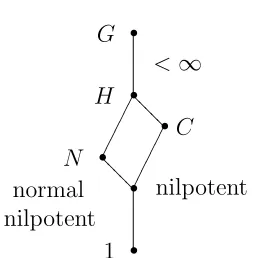
Theorem 2.5.4. Let G be a polycyclic group. Then there exists a normal
T-subgroup N and aT-subgroup C such that CN/N is free abelian andCN
has finite index in G.
Definition 2.5.5. The group C from Theorem 2.5.4 is said to be a nilpo-tent almost-supplement for N in G. ‘Almost’ because C and N generate a subgroup of finite index, and ‘supplement’ because C may intersect N
non-trivially.
This structure of polycyclic groups can also be explored algorithmically. Let G be a polycyclic group given by a polycyclic presentation. In [17, Chapter 9] Eick describes a practical algorithm to compute a nilpotent-by-abelian-by-finite series G ≥ K ≥ N ≥ 1 where K is torsion-free. The algorithm computes generators for K andN as words in the generators ofG; it also computes polycyclic presentations for K and N on these generators. Further, Eick describes methods to determine a nilpotent almost-supplement
C for N in G. Since [G:CN]<∞ we can impose the additional condition that CN is normal in G by passing to the core (CN)G of CN in G. Note
Chapter 3
Mal’cev correspondence
In this chapter we recall some well known facts about the connection be-tween Q-powered nilpotent groups and rational nilpotent Lie algebras, the Mal’cev correspondence, discovered by Anatoly Mal’cev in 1951 [27, 28]; this correspondence plays a key role in the further chapters of this book.
In§3.1 we defineQ-powered groups and give some basic facts about Lie al-gebras. In§3.2 we study an illustrative special case of the Mal’cev correspon-dence: the connection between upper unitriangular rational matrix groups and nilpotent rational matrix Lie algebras. Then in §3.3 we move on to the general case where the Mal’cev correspondence between abstract groups and Lie algebras is realized by means of the Baker–Campbell–Hausdorff formula. For more background we refer to [9, Chapter 4], [23, Chapter 9,10] and [38, Chapter 6],
3.1
Preliminaries
Q
-powered groups
Definition 3.1.1. A group G is said to be Q-powered if for every g ∈ G,
q∈N there exists a unique h∈Gsuch thathq =g. We denote this element
h by g1q and write g p q for (g
1
q)p where p∈Z, q∈N.
If G isQ-powered then gq = 1 implies g = 1; thusG is torsion-free.
Definition 3.1.2. We denote by Tr1(d,Q) the group of all upper unitrian-gular matrices of degree n over Q, i.e. matrices of the form
1 ∗
. ..
0 1
.
26 Chapter 3. Mal’cev correspondence
Example 3.1.3. Let g =
1 x
0 1
∈ Tr1(2,Q) and n ∈ N. Then h =
1 x/n
0 1
is the unique element in Tr1(2,Q) such that hn = g. Thus
Tr1(2,Q) is a Q-powered group. We will see in §3.2 that Tr1(d,Q) is Q -powered for all d∈N.
Note that Tr1(d,Q) is a nilpotent group [38, Chapter 1]. Furthermore every T-group, i.e. a finitely generated torsion-free nilpotent group, can be embedded in some Tr1(d,Q) [38, Chapter 5].
Lie algebras
Definition 3.1.4. LetLbe a vector space over a fieldK. ThenLis said to be aLie algebraif there exists a bilinear mapL×L→L, written (x, y)7→[x, y], with the properties
(1) [x, x] = 0, (2) [x, y] =−[y, x],
(3) [[x, y], z] + [[y, z], x] + [[z, x], y] = 0.
The expression [x, y] is called aLie commutator or a Lie bracket inx and y. Equation (3) is the Jacobi identity. A vector subspace V ≤L is called aLie subalgebra if it is closed under the Lie bracket, i.e. [V, V]≤V.
For repeated Lie brackets we use the left norm convention, i.e.
[x1, . . . , xr] = [[x1, . . . , xr−1], xr].
Example 3.1.5. Denote by Mn×n(Q) the set of all rational matrices of degree
n. Then Mn×n(Q) is a Lie algebra with Lie bracket [x, y] =xy−yx.
Definition 3.1.6. LetL be Lie algebra. Thelower central series(Lk)k∈N of
L is recursively defined by L1 =L and Lk+1 = [Lk, L]. The Lie algebra L is
said to be nilpotent if Lc = 0 for somec∈N. A nilpotent Lie algebra L has
nilpotency class cif Lc+1 = 0 andLc 6= 0.
Definition 3.1.7. Let L be Lie algebra. The center of L is defined by
Z(L) = {l ∈ L|[l, L] = 0}. Note that Z(L) is a vector subspace of L. The upper central series (Lk)
k∈N of L is recursively defined by L1 = Z(L) and
Lk+1/Lk =Z(L/Lk).
3.2. Matrix correspondence 27
Definition 3.1.8. We denote by Tr0(d,Q)≤ Mn×n(Q) the vector subspace
of all upper triangular matrices with zeros on the diagonal. Since Tr0(d,Q) is closed under the Lie bracket [x, y] =xy−yx we see that Tr0(d,Q) is a Lie subalgebra of Mn×n(Q).
Tr0(d,Q) is nilpotent because the kth term of the lower central series consists of matrices of the form
0 . . . 0 ∗
. .. . ..
. .. 0
. .. ...
0 0
where the k−1 subdiagonals above the diagonal are equal to 0.
Definition 3.1.9. Let L be a Lie algebra over a field K and let B =
{x1, . . . , xn}be a basis of the underlying vector space. For each pairxi, xj ∈
B we can write
[xi, xj] = n
X
k=1
ckijxk.
The n3 elements ck
ij ∈K are called thestructure constantsof L with respect
to B. Since the Lie bracket [,] in L is bilinear, it is completely specified by the structure constants.
Finite dimensional Lie algebras are typically represented on a computer via matrices or via a structure constant table. In the first case the Lie algebra is given by a basis consisting of matrices{X1, . . . , Xn}; in the second case the
Lie algebra is given as an abstract vector space with basis B ={x1, . . . , xn}
and the structures constants with respect to B. For both representations, which can be obtained from each other, powerful algorithms for structural investigations are available [12]. Note that every finite dimensional Lie alge-bra has a faithful linear representation [21].
3.2
Matrix correspondence
Recall that we denote by Tr1(d,Q) the group of all upper unitriangulard×d -matrices over Q, and by Tr0(d,Q) the Lie algebra of all upper triangular
28 Chapter 3. Mal’cev correspondence
Definition 3.2.1. We define the maps log and the exp as follows:
log : Tr1(d,Q)→Tr0(d,Q)
: g 7→(g −1)− 1
2(g−1)
2+· · ·+ (−1)d
(d−1)(g−1)
d−1
exp : Tr0(d,Q)→Tr1(d,Q)
: x7→1 +x+1 2x
2+· · ·+ 1 (d−1)!x
d−1
Note that this coincides with the usual definition of log and exp on the complex numbers via power series, since (g −1)d = xd = 0. The following
lemma is a consequence of well-known identities of these power series.
Lemma 3.2.2. The mappings log and exp from Definition 3.2.1 are mutu-ally inverse bijections. For commuting matrices x, y ∈ Tr0(d,Q), we have (expx)(expy) = exp(x+y).
Remark 3.2.3. For q ∈ N and g = exp(x) ∈ Tr1(d,Q) we have that h = exp(1
qx) is a q-th root of g, i.e. h
q = g. Since hq = kq implies qlog(h) =
qlog(k) and thush=k, we deduce thathis a uniqueq-th root ofg. Therefore Tr1(d,Q) is a Q-powered group. For r∈Q we have that
log(gr) = rlog(g) exp(rx) = exp(x)r.
For non-commuting matrices x, y ∈ Tr0(n,Q) it is not true in general that exp(x+y) = exp(x) exp(y). However a similar equality holds which contains additional error terms which depend on the extent to which x and
y fail to commute. For a vector of positive integerse = (e1, . . . , er) we define
the repeated Lie bracket [x, y]e in Tr0(d,Q) by
[x, y]e= [x, y, . . . , y
| {z }
e1
, x, . . . , x
| {z }
e2
, . . .].
Theorem 3.2.4. There exist constants qe ∈Q not depending on d such that
for all x, y ∈Tr0(d,Q) we have
exp(x) exp(y) = exp(x+y+X
e
qe[x, y]e),
where we take the sum over all vectors e = (e1, . . . , er), with positive
inte-ger entries, such that e1 +· · ·+er < d−1. In particular this means that
3.2. Matrix correspondence 29
Proof. See [23, Section 9.2] and [38, Chapter 6].
Definition 3.2.5. Let the rational constants qe be defined as in the last
theorem. The formal expression H(x, y) = x+y+Peqe[x, y]e, where the
sum is taken over all vectors (e1, . . . , er) with positive integer entries where
r∈N, is called the Baker–Campbell–Hausdorff formula.
Remark 3.2.6. IfL is a nilpotent Lie algebra of nilpotency class c then any Lie bracket of length c+ 1 in x, y ∈ L is trivial. Thus in L the Baker– Campbell–Hausdorff formulaH(x, y) has only finitely many non-zero terms.
Example 3.2.7. The terms up to length 3 of the Baker–Campbell–Hausdorff formula are
H(x, y) =x+y+1
2[x, y] +− 1
12[x, y, y] + 1
12[x, y, x] +. . .
Theorem 3.2.8. We can define a group multiplication ∗ onTr0(d,Q) given by x∗y =H(x, y). The exponential map is then an isomorphism of groups between (Tr0(d,Q),∗) and Tr1(d,Q).
Proof. Let x ∈ Tr0(d,Q). From the definition of ∗ we see that 0∗ x =
x∗ 0 = x and that −x is an inverse of x. By Lemma 3.2.2 the function exp : Tr0(d,Q) → Tr1(d,Q) is a bijection. Further, by Theorem 3.2.4, we have that exp(x∗y) = exp(x) exp(y) for x, y ∈Tr0(d,Q), which implies the associativity of ∗ and that exp is an isomorphism.
The following theorem explains the interplay of subgroups of Tr1(d,Q) and Lie subalgebras of Tr0(d,Q) via log and exp.
Theorem 3.2.9. Let G ≤Tr1(d,Q) and let Qlog(G) be the Q-vector space spanned by log(G) ={log(g)|g ∈G}. Let L be a Lie subalgebra of Tr0(d,Q). Then the following holds:
• exp(L) is a Q-powered nilpotent subgroup of Tr1(d,Q).
• Qlog(G) is a Lie subalgebra of Tr0(d,Q).
• G≤exp(Qlog(G)) and every element of exp(Qlog(G)) has some pos-itive power lying in G.
Proof. See [38, Chapter 6, Theorem 2].
30 Chapter 3. Mal’cev correspondence
Theorem 3.2.9 shows that exp(Qlog(G)) is a Q-powered hull of a sub-group G≤Tr1(d,Q); further ifG is Q-powered thenG= exp(Qlog(G)).
We saw that the Baker–Campbell–Hausdorff formula allows us to define a group multiplication on Tr0(d,Q) in terms of Lie algebra operations. Vice versa, it is possible to define operations of a Lie algebra on Tr1(d,Q) in terms of the operations of a Q-powered group.
For a vector of positive integers e = (e1, . . . , er) we define the repeated
group commutator [g, h]e in Tr1(d,Q) by [g, h]e = [g, h, . . . , h
| {z }
e1
, g, . . . , g
| {z }
e2
, . . .].
The weight w(e) ofe is defined to be Pri=1ei. Let ≤ be an order on a set of
vectors with positive integer entries. We say that≤ agrees with the increase of the weight of the vectors if e≤e′ implies w(e)≤w(e′).
Theorem 3.2.11. There exist constants re, se∈Q not depending on d such
that for all g, h∈Tr1(d,Q)
log(g) + log(h) = log(ghY
e
[g, h]ere)
[ log(g),log(h)] = log([g, h]Y
e
[g, h]ese)
where the product is taken over all vectors e = (e1, . . . , er), with positive
integer entries, such that e1 +· · ·+er < d−1 in some fixed order agreeing
with the increase of the weight of the vectors e.
Proof. See [23, Section 10.1].
Definition 3.2.12. Let the rational constants re and se be defined as in the
last theorem. The formal expressions
h1(g, h) = gh
Y
e
[g, h]ere
h2(g, h) = [g, h]
Y
e
[g, h]ese,
where the product is taken over all vectors e = (e1, . . . , er) with positive
integer entries where r ∈N in some fixed order agreeing with the increase of the weight of the vectorse, are called the inverse Baker–Campbell–Hausdorff formulae.
Remark 3.2.13. If G is a Q-powered nilpotent group of nilpotency class c
then any group commutator of length c+ 1 in g, h∈G is trivial. Thus in G
3.3. Abstract correspondence 31
3.3
Abstract correspondence
We now describe the Mal’cev correspondence between abstract Q-powered nilpotent groups and abstract rational nilpotent Lie algebras.
LetLbe a nilpotent Lie algebra overQand letx, y ∈L. Using the Baker– Campbell–Hausdorff formulaH(x, y) from Definition 3.2.5 we can define the operations of a Q-powered group on L by
x∗y = H(x, y) (3.1)
xq = qx for q ∈Q. (3.2)
Conversely, let G be a Q-powered nilpotent group and let g, h ∈ G. Then using the inverse Baker–Campbell–Hausdorff formulaeh1(g, h), h2(g, h) from Definition 3.2.12 we can define the operations of a rational Lie algebra on G
by
g+h = h1(g, h) (3.3)
[g, h] = h2(g, h) (3.4)
qg = gq for q ∈Q. (3.5)
Theorem 3.3.1 (Mal’cev correspondence). For every Q-powered nilpotent group G, the corresponding rational nilpotent Lie algebra LG is defined on
the same underlying set LG=G, with Lie Q-algebra operations (3.3), (3.4),
(3.5). Conversely, for every rational nilpotent Lie algebra L, the correspond-ing Q-powered nilpotent group GL is defined on the same underlying set
GL = L, with group operations (3.1), (3.2) of a Q-powered group. These
transformations are inverses of one another: LGL = L as rational Lie
al-gebras (that is, not only sets, but all operations coincide), and, similarly,
GLG =G as (Q-powered) groups.
Proof. See [23, Theorem 10.11.].
Let G be a Q-powered nilpotent group. To avoid confusion between G
and LG in the following, we will denote by Log(g) the element of LG which
corresponds to g ∈G;
G∋g ↔ Log(g)∈LG = Log(G) ={Log(g)|g ∈G}.
For a rational nilpotent Lie algebraL we will denote by Exp(x) the element of GL which corresponds to x ∈ L. Distinguishing G and LG in this way,
32 Chapter 3. Mal’cev correspondence
commutator or the group commutator. Log can be regarded as a mapping between G and Log(G). For g, h∈G and q ∈Qwe have
Log(gh) = Log(g)∗Log(h) Log(h1(g, h)) = Log(g) + Log(h) Log(h2(g, h)) = [Log(g),Log(h)]
Log(gq) = qLog(g).
Similarly Exp can be regarded as a mapping between L and Exp(L).
Remark 3.3.2. Note that in the context of the matrix Mal’cev correspondence as discussed in §3.2 we use log to denote the function
log : Tr1(d,Q)→Tr0(d,Q)
: g 7→(g−1)− 1
2(g−1)
2+· · ·+ (−1)d
(d−1)(g−1)
d−1
which links theQ-powered nilpotent matrix group Tr1(d,Q) and the nilpotent Lie algebra Tr0(d,Q). In opposition to this we use in the context of the abstract Mal’cev correspondence the function name Log to link an abstract nilpotent Q-powered group Gand the corresponding Lie Algebra LG.
LetH be a torsion-free nilpotent group. Recall that a Q-powered group ˆ
H, containing H, is said to be a Q-powered hull of H, if for every element
h∈Hˆ there exists z ∈N such that hz ∈H.
Theorem 3.3.3. Let H be a torsion-free nilpotent group. ThenH has a Q -powered hull Hˆ of the same nilpotency class. If Hˆ1,Hˆ2 are Q-powered hulls of H then the identity map inH extends to a unique isomorphism ofHˆ1 onto
ˆ
H2. Every automorphism ofH extends to an automorphism ofHˆ. If H ≤G and G isQ-powered, then G contains a Q-powered hull of H.
Proof. See [23, Corollary 9.19. and Theorem 9.20.]
Given the fact that all Q-powered hulls of a torsion-free nilpotent group
H are isomorphic, we will identify them in the following and speak of the
Q-powered hull ˆH of H. The Lie algebra LHˆ corresponding to ˆH will be denoted by L(H). Note that L(H) is spanned by Log(H) ⊆ L(H) over the rationals, because every element h ∈Hˆ has some power hz lying in H; thus
3.3. Abstract correspondence 33
Remark 3.3.4. LetN be aT-group and β:N →Tr1(d,Q) a faithful matrix representation. By§3.2, L=Qlog(Nβ) is a Lie algebra and exp(L)∼= (L,∗) is aQ-powered hull ofN. By Theorem 3.3.3, (L,∗) and (L(N),∗) are isomor-phic asQ-powered nilpotent groups and thus, by the Mal’cev correspondence,
L and L(N) are isomorphic as rational Lie algebras.
In Chapters 5, 6 and 7 we will use the Mal’cev correspondence for com-putations with automorphisms of a T-group H. The next theorem shows that the automorphisms of ˆH and L(H) are in one-one correspondence; it is a direct consequence of the fact that the Lie algebra operations in L(H) can be defined in terms of the group operations of ˆH and vice versa.
Theorem 3.3.5. Let G be a Q-powered nilpotent group and L its corre-sponding Lie algebra. Then the map ˜ : Aut(G) → Aut(L), defined by
ϕ7→ Exp◦ϕ◦Log is an isomorphism.
Proof. Letϕ ∈Aut(G) and g, h∈G. Then
(Log(g) + Log(h))ϕ˜ = Log(h
1(g, h))ϕ˜ = Log(h1(g, h)ϕ) = Log(h1(gϕ, hϕ)) = Log(gϕ) + Log(hϕ) = Log(g)ϕ˜+ Log(h)ϕ˜.
With a similar argument we see that [Log(g),Log(h)]ϕ˜ = [Log(g)ϕ˜,Log(h)ϕ˜] and that for q ∈ Q we have (qLog(g))ϕ˜ = q(Log(g)ϕ˜. Thus ˜ϕ ∈ Aut(L) because by the properties of the Mal’cev correspondence for every x, y ∈ L
there exist g, h ∈G such that Log(g) =x and Log(h) =y.
Similarly we see that for τ ∈ Aut(L), the mapping Log◦τ ◦Exp is in Aut(G). Therefore, since ϕ 7→ Exp◦ϕ ◦Log and τ 7→ Log◦τ ◦Exp are inverses of each other, ˜ is a bijection between Aut(G) and Aut(L). Further for ϕ, ψ∈Aut(G) we have thatϕψf = ˜ϕψ˜and thus ˜ is an isomorphism.
The next theorem explains how Aut(H) fits into the relationship between the automorphism group of ˆH and L(H).
Theorem 3.3.6. LetHbe a torsion-free nilpotent group andHˆ itsQ-powered hull. Let Γ be the setwise stabilizer in Aut(L(H)) of the set Log(H). Then
ϕ ∈ Aut( ˆH) induces an automorphism of H, i.e. Hϕ = H, if and only if ˜
ϕ∈ Γ.
Proof. Letϕ ∈Aut( ˆH) and assume thatHϕ=H. Then we have Log(H)ϕ˜ = Log(Hϕ) = Log(H). Thus ˜ϕ ∈ Γ. Conversely assume that ˜ϕ ∈ Γ. Then
34 Chapter 3. Mal’cev correspondence
Lemma 3.3.7. Denote by x1, . . . , xs abstract Lie elements. Let K be the
set of all repeated Lie brackets κ(x1, . . . , xs) of length at least s+ 1 in the
arguments x1, . . . , xs each of which appears at least once. Then there exist
rational constants(tκ)κ∈K such that for anyQ-powered nilpotent groupGand
g1, . . . , gs∈G it holds that
[Log(g1), . . . ,Log(gs)] =
Log([g1, . . . , gs]) +
X
κ∈K
tκκ(Log(g1), . . . ,Log(gs)). (3.6)
Proof. See [38, Chapter 6, Corollary 2].
Remark 3.3.8. The sum in equation (3.6) is by definition infinite. However for a given Q-powered nilpotent group G only a finite number of the Lie brackets κ are nonzero.
Lemma 3.3.9. Denote by x1, . . . , xs abstract group elements. Let L be the
set of all repeated group commutators λ(x1, . . . , xs) of length at least s + 1
in the arguments x1, . . . , xs each of which appears at least once. Then there
exist rational constants (uλ)λ∈L such that for any Q-powered nilpotent group
G and g1, . . . , gs∈G it holds that
[Log(g1), . . . ,Log(gs)]
= Log([g1, . . . , gs]) +
X
λ∈L
uλLog(λ(g1, . . . , gs)). (3.7)
Proof. By Lemma 3.3.7 we have
[Log(g1), . . . ,Log(gs)] =
Log([g1, . . . , gs]) +
X
κ∈K
tκκ(Log(g1), . . . ,Log(gs)). (3.8)
Now we replace all occurrences of Lie brackets of length ≥s+ 1 in (3.8) with the corresponding right hand side of (3.6) and continue until no Lie bracket of length ≥s+ 1 appears in the equation.
This process must stop, becauseG and L(G) have finite nilpotency class
cand thus group commutators and Lie brackets of lengths greater then care trivial, and because a replacement of a Lie bracket of lengthkonly introduces Lie brackets of length ≥k+ 1.
The only influence of the groupGon this process is its nilpotency classc, which tells us that group commutators and Lie brackets of length c+ 1 can be disregarded. However this does not affect the values of those uλ whose
corresponding λ is of length ≤ c. Thus the constants uλ are not depending
3.3. Abstract correspondence 35
Remark 3.3.10. The sum in equation (3.7) is by definition infinite. However for a given Q-powered nilpotent group G only a finite number of the group commutators λ are nontrivial.
Remark 3.3.11. [38, Chapter 6, Corollary 3] claims that the constants uλ in
the last lemma depend onc.
Lemma 3.3.12. Let (g1, . . . , gl) be a Mal’cev basis for a T-group H. Then
B={Log(g1), . . . ,Log(gl)}is a basis for the Lie algebra L(H). In particular,
the dimension of L(H) is equal to the Hirsch length of H.
Proof. Let g = ga1 1 · · ·g
al
l ∈ H. Then Log(g) = a1Log(g1)∗ · · · ∗alLog(gl).
Thus L(H) is generated by B as a Lie algebra, i.e. the smallest Q-vector space that contains B and is closed under taking Lie brackets is equal to
L(H).
We show via induction over l, the Hirsch length of H, that B is a basis of L(H).
If H = hg1i then {Log(g1)} is a basis for L(H). Assume that the lemma is true for all T-groups of Hirsch length l−1. First we show that the Q-span hBiQ of B is equal to L(H). By assumption the vector spaces
hLog(g2), . . . ,Log(gl)iQ andhLog(g1),Log(g3), . . . ,Log(gl)iQare closed under
taking Lie brackets. Thus we have to show that [Log(g1),Log(g2)]∈ hBiQ. By
Lemma 3.3.9 [Log(g1),Log(g2)] = Log([g1, g2]) +PuλLog(λ(g1, g2)), where
uλ ∈ Q and λ is a repeated group theoretic commutator in g1, g2 of length
≥3. Since [g1, g2], λ(g1, g2)∈ hg3, . . . , glithe right hand side of the last
equa-tion is contained in the Lie algebra L(hg3, . . . , gli) and thus in the Q-vector
space spanned by B.
It remains to show that the elements ofBare linearly independent. By the induction hypothesis Log(g2), . . . ,Log(gl) are linearly independent. So
as-sume that Log(g1) ∈ hLog(g2), . . . ,Log(gl)iQ = L2. Therefore g1 ∈ Exp(L2) which is equal to the Q-powered hull of hg2, . . . , gli. Thus there must be an
m ∈ N such that gm
1 ∈ hg2, . . . , gli. Since (g1, . . . , gl) is a Mal’cev basis this
Chapter 4
Computing the correspondence
In this chapter we show how the Mal’cev correspondence between the radi-cable hull of a T-groupGand the Lie algebra L(G) can be set up on a com-puter. We assume that G is given by a polycyclic presentation with respect to a Mal’cev basis G = (g1, . . . , gl). Note that B={Log(g1), . . . ,Log(gl)} is
a basis of L(G). We show how to solve the following three tasks:
• Lie algebra presentation: Determine a computer presentation of
L(G).
• Logarithm: Given an elementg =ge1 1 · · ·g
el
l ∈Gˆ, compute the
coeffi-cient vector (α1, . . . , αl) such that Log(g) =Pli=1αiLog(gi).
• Exponential: Given an element x = Pli=1αiLog(gi) ∈ L(G),
com-pute the exponent vector (e1, . . . , el) such that Exp(x) =g1e1· · ·gell.
We present two approaches for solving these tasks. The first uses the fact that every T-group can be embedded in an upper unitriangular matrix group and is discussed in§4.1. The second makes use of the Baker–Campbell–Hausdorff formula and related identities, see§4.2. Further we present in§4.3 a symbolic approach for computing logarithms and exponentials. Finally, we compare these methods and report on their implementations in §4.4.
4.1
Via matrix embeddings
This method uses a vector subspace of Tr0(d,Q) to represent L(G) on a computer.
Every T-group G has a faithful matrix representation β :G→Tr1(d,Q) for some d ∈ N [38, Chapter 3]. Recall that by Remark 3.3.4 the Lie al-gebra Qlog(Gβ), i.e. the Q-vector space spanned by log(Gβ), is isomorphic
4.1. Via matrix embeddings 37
to L(Gβ) and thus to L(G). For a T-group G, given by a polycyclic pre-sentation, it is possible to compute β : G → Tr1(n,Q) [13, 26, 33]. An implementation of [13] is publicly available as part of GAP [41].
In order to be able to go back and forth betweenGandGβ, it is necessary to compute a special kind of polycyclic sequence for Gβ.
Definition 4.1.1. A polycyclic sequence M = (M1, . . . , Ml) for a finitely
generated groupH ≤Tr1(n,Q) is calledconstructiveif there exists a practical algorithm which, given any h ∈ H, determines the normal form nf(h) with respect to M.
It is well-known how to compute a constructive polycyclic sequence for a given finitely generated groupH ≤Tr1(n,Q) which is also a Mal’cev basis of
H, see for example [39, Chapter 9]. By changing the underlying generating set of the polycyclic presentation of G, we can assume in the following that
G = (g1, . . . , gl) is a polycyclic sequence of G such that (g1β, . . . , glβ) is
constructive polycyclic sequence and Mal’cev basis for Gβ. As a basis for
L(G)∼=Qlog(Gβ) we use the set of matrices (log(g1β), . . . ,log(glβ)).
The task Logarithm can be solved as follows. Giveng =ge1 1 · · ·g
el
l ∈Gˆ, we
compute M = (g1β)e1· · ·(glβ)el and then log(M). Finally, by solving linear
equations, we determine (α1, . . . , αl) such that Pαilog(giβ) = log(M).
For the task Exponential we do the following. Givenx=Pli=1αilog(giβ),
we compute exp(x). Then we can use the constructive polycyclic sequence (g1β, . . . , glβ) ofGβ to compute the exponent vector (e1, . . . , el) of exp(x) as
described in [39, Chapter 9].
Example 4.1.2. Let G = F2,2 be the free nilpotent of class two group on two generators g1, g2. Then the derived group is cyclic and generated by
g3 = [g2, g1]. It follows that
G=hg1, g2, g3|g(g
±1 1 )
2 =g2g3±1i
is a polycyclic presentation for GandG = (g1, g2, g3) is a Mal’cev basis. The embedding β→Tr1(3,Q), as computed by the algorithm in [13], is given by
g1β =
1 0 00 1 1 0 0 1
, g2β =
10 −11 00
0 0 1
, g3β=
1 00 1 −01
0 0 1
.
38 Chapter 4. Computing the correspondence
and set M= (g1β, g2β, g3β). The corresponding basis of Qlog(Gβ)∼=L(G) consists of
log(M1) =
0 0 00 0 1 0 0 0
,log(M2) =
00 −01 00
0 0 0
,log(M3) =
0 00 0 −01
0 0 0
.
Let x = log(M1) + log(M2) + log(M3)∈ L(G) and assume that we want to compute the exponent vector of Exp(x), i.e. the vector (e1, e2, e3) such that
(ge1
1 g2e2g3e3)β = exp(x). First we compute
exp(x) = x 0 0! + x1 1! + x2 2! =
10 −11 −31/2
0 0 1
Now we can read off from the first subdiagonal thate1 = 1 and e2 = 1. Next we divide off and compute
(g3β)e3 = ((g1β)e1(g2β)e2)−1exp(x) =
1 00 1 −30/2
0 0 1
.
This implies e3 = 3/2.
4.2
Via the Baker–Campbell–Hausdorff
formula
This method uses an abstract vector space and a structure constant table with respect to the basis B to present L(G) on a computer.
For the computation of the structure constants, we use equation (3.7) from Lemma 3.3.9; it expresses [Log(g),Log(h)], whereg, h∈G, in terms of a linear combination of logarithms of group commutators.
The proof of Lemma 3.3.9 is constructive and therefore can be used to compute the terms of (3.7); it makes use of the equation (3.6) from Lemma 3.3.7, whose terms can be determined using the method in [36, §8] and the Dynkin bracket operator defined in [44, Chapter 2].
Example 4.2.1. With [Log(g),Log(h)] as left hand side, equation (3.6) is
[Log(g),Log(h)] = Log([g, h]) + 1
2[Log(h),Log(g),Log(h)]
+1
4.2. Via the Baker–Campbell–Hausdorff formula 39
where only terms up to length 3 are displayed. Now we replace all Lie brackets of length ≥3 by the according right hand side of (3.6) and get
[Log(g),Log(h)] = Log([g, h]) + 1
2Log([h, g, h]) + 1
2Log([h, g, g]) +. . . This is equation (3.7) with [Log(g),Log(h)] as left hand side, where only terms up to length 3 are displayed.
Note that the terms of equation (3.6) and equation (3.7) do not depend onG. Therefore they can be precomputed up to a given length. The number of terms grows exponentially in the length.
Let G = (g1, . . . , gl) be a Mal’cev basis of G and denote by B the
corre-sponding basis {Log(g1), . . . ,Log(gl)} of L(G). We show by induction on l
that it is possible to compute the structure constant table of the Lie algebra
L(G) with respect to B.
If l = 1, then L(G) is abelian and so the structure constant table of B
is known. If l > 1, then we can assume by induction that the structure constant table of {Log(g2), . . . ,Log(gl)} is already known and that we can
compute Log(g) forg in theQ-powered hull ofhg2, . . . , gli. Then using (3.7),
we can express [Log(g1),Log(gi)] as a linear combination of logarithms of
repeated group commutators κ(g1, gi). Since κ(g1, gi) is in hg2, . . . , gli for
any commutator κ, we can compute Log(κ(g1, gi)) and therefore determine
the coefficients of [Log(g1),Log(gi)] with respect toB. Thus we can compute
the structure constant table of B.
For the computation of Logarithms we use the fact that Log(gh) = Log(g)∗Log(h). Thus for given g = ge1
1 · · ·g el
l ∈ Gˆ we have that Log(g) =
(e1Log(g1)) ∗ · · · ∗(elLog(gl)), and therefore the coefficients of Log(g) =
P
αiLog(gi) can be be computed by using the Baker–Campbell–Hausdorff
formula and the structure constant table of B.
It remains to solve the task Exponential. For a given element x =
Pl
i=1αiLog(gi) ∈ L(G) we have that x = (α1Log(g1))∗(−α1Log(g1))∗x and y = (−α1Log(g1))∗x ∈ hLog(g2), . . . ,Log(gl)iQ. Thus e1 = α1. Us-ing the structure constant table of B and the BCH-formula we can compute
y := (−α1Log(g1))∗x. By induction on l, we can assume that we can de-termine f2, . . . , fl such that g2f2· · ·g
fl
l = Exp(y). Since Exp(x) =g α1
1 Exp(y) we deduce that (e1, . . . , el) = (α1, f2, . . . , fl).
Example 4.2.2. Let G= F2,2 be given as in Example 4.1.2. We have that [Log(e),Log(f)] = Log([e, f]) for e, f ∈ G. Therefore [Log(g2),Log(g1)] = Log(g3) and [Log(g3),Log(g1)] = [Log(g3),Log(g2)] = 0.
Let g = g1g25 and suppose that we want to compute the coefficients of Log(g). We have that Log(g) = Log(g1)∗Log(g25) = Log(g1) + 5 Log(g2) +
1
2[Log(g1),5 Log(g2)]. Thus Log(g) = Log(g1) + 5 Log(g2)− 5
40 Chapter 4. Computing the correspondence
4.3
Symbolic
Log
and
Exp
It is well-known that, in the context of T-groups, Log and Exp can be de-scribed by polynomial functions [22, Chapter 6]. In this section we show how to compute these functions and apply them for the computations of logarithms and exponentials.
Lemma 4.3.1. Let G be a T-group with Mal’cev basis G= (g1, . . . , gl).
(i) Define l functions α1, . . . , αl in l rational variables e1, . . . , el such that
l
X
i=1
αiLog(gi) = Log(g1e1· · ·g el
l ).
Thenαi is a polynomial in e1, . . . , el for i= 1, . . . , l.
(ii) Define l functions e1, . . . , el in l rational variables α1, . . . , αl such that
ge1 1 · · ·g
el
l = Exp
l
X
i=1
αiLog(gi)
!
.
Thenei is a polynomial in α1, . . . , αl fori= 1, . . . , l.
Proof. (i): Let x = Pli=1riLog(gi), y = Pli=1siLog(gi) ∈ L(G). By
the properties of the Baker–Campbell–Hausdorff formula the coefficients of
x ∗ y with respect to the basis {Log(g1), . . . ,Log(gl)} are polynomials in
r1, . . . , rl, s1, . . . , sl.
Forg =ge1
1 · · ·glel we have that Log(g) = (e1Log(g1))∗ · · · ∗(elLog(gl)).
By the repeated application of the argument from above we see that αi is a
polynomial in e1, . . . , el for i= 1, . . . , l.
(ii): Let x=Pli=1αiLog(gi)∈ L(G). If l= 1, then e1(α1) =α1 and thus e1 is a polynomial. Now assume that l > 1. In §4.2 we saw that (e1, . . . el) =
(α1, f2, . . . , fl) where g2f2· · ·g fl
l = Exp(y) with y = (−α1Log(g1))∗x. Let
y = Pli=2βiLog(gi). By the properties of the Baker–Campbell–Hausdorff
formula βi is a polynomial inα1, . . . , αl. Further by induction we can assume
that f2, . . . , fl are polynomials in β2, . . . , βl. Thus ei is a polynomial in
α1, . . . , αl fori= 1, . . . , l.
Example 4.3.2. Let G = F2,2 be the group already studied in Example 4.1.2 and 4.2.2. We have that
Log(ge1 1 g
e2 2 g
e3
3 ) = (e1Log(g1))∗(e2Log(g2))∗(e3Log(g3))
4.4. Runtimes and comparison 41
The proof of the Lemma 4.3.1 is constructive and can be used to compute the polynomials αi and ej if the structure constant table of the Lie algebra
L(G) is known. See§4.4 for comments on the implementation and runtimes. The functions αi, ej can be applied for the computation of logarithms
and exponentials. In §4.4 we will see that this is yields a considerable speed up in comparison with the methods described in §4.1 and 4.2.
4.4
Runtimes and comparison
The approaches described in §4.1, §4.2 and §4.3 to realizing the Mal’cev correspondence have been implemented in GAP [41] as a part of the package Guarana [2]. In this section we make comments on their implementation, indicate runtimes and compare them.
Implementation
For the method of§4.1, we used the algorithm and implementation of Nickel [33] to compute the faithful matrix representations of the given T-group G. It is much more efficient than previous methods [13, 26].
For the method of §4.2, we use a weight function that can be associated to every Mal’cev basis G = (g1, . . . , gl); this is a function w : G → N\{0}
such that for all gk showing up in the normal form of [gi, gj] we have that
w(gk)≥w(gi)+w(gj). If ¯w= maxw(G) then [gi, gj] = 1 ifw(gi)+w(gj)>w¯;
more generally a group commutator ingi andgj withα occurrences ofgi and
β occurrences of gj is equal to 1 if αw(gi) +βw(gj) > w¯. The equivalent
fact holds in the corresponding Lie algebra. A Lie commutator in Log(gi)
and Log(gj) with α occurrences of Log(gi) and β occurrences of Log(gj)
is equal to zero if αw(gi) +βw(gj) > w¯. This can be used to reduce the
number of commutators which have to be evaluated during the computation of Log(gi)∗Log(gj).
For the method of§4.3 for computing Log and Exp, we use the structure constant table of the Lie algebra L(G) as computed by the method of §4.2. Further the terms of the BCH-formula are determined using [36,§8] and the Dynkin bracket operator defined in [44, Chapter 2].