RIPPLE COMPENSATION FOR A CLASS-D AMPLIFIER∗
STEPHEN M. COX† AND H. DU TOIT MOUTON‡
Abstract. This paper presents the first detailed mathematical analysis of the ripple compen-sation technique for reducing audio distortion in a class-D amplifier with negative feedback. The amplifier converts a relatively low-frequency audio signal to a high-frequency train of rectangular pulses whose widths are slowly modulated according to the audio signal (pulse-width modulation, PWM). Distortion manifests itself through unwanted audio-frequency harmonics that arise in the output due to nonlinearities inherent in the design. In this paper, we first develop a small-signal model, which describes the fate of small-amplitude perturbations to a constant input, and demon-strate how this traditional engineering tool may be extended to allow one to infer the most significant contributions to the full output in response to a general audio input. We then compute the audio output of the amplifier through a perturbation expansion based on the ratio between audio and switching frequencies. Our results explicitly demonstrate how the ripple compensation technique significantly linearizes the output, thereby reducing the distortion.
Key words. class-D amplifier, mathematical model, small-signal model, Apostol–Bernoulli functions, pulse-width modulation
AMS subject classifications.33E30, 34E10, 37N20
DOI.10.1137/140997695
1. Introduction. Class-D amplifiers are a technologically significant application of switching electronics. An audio signal (of relatively low frequency) is converted by a class-D amplifier to a high-frequency rectangular wave. The latter wave generally has a fixed frequency but a duty cycle that is modulated slowly according to the audio signal (the duty cycle being the proportion of time the output is “on”). The conversion from audio signal to rectangular wave is called pulse-width modulation (PWM) [3, 8]. The modulation is carried out with the intention that the low-frequency content of the modulated rectangular wave should faithfully reproduce the original audio signal. In practice, however, there are many sources of potential distortion in the out-put. One of particular significance follows from the fact that the output rectangular wave switches between the voltages at the power supply rails, and hence any low-frequency ripple in the power supply may become audible in the output. To mitigate such effects, the class-D amplifier generally includes some form of negative feedback. Unfortunately, nonlinearities in the PWM process, coupled to the negative feedback, generate unwanted additional audio components in the output. It is the goal of the amplifier designer to reduce such distortion, and over the years many techniques have been proposed and adopted to reduce output distortion in class-D amplifiers [2, 4, 15]. Recently, the technique ofripple compensation [12, 14] (henceforth RC) has been introduced and found to dramatically reduce audio distortion in class-D amplifiers. This paper presents the first detailed mathematical analysis of RC, which enables us to quantify its notable effectiveness in suppressing nonlinearities in the output. Our analysis is presented for arguably the simplest possible amplifier design, to clarify
∗Received by the editors November 26, 2014; accepted for publication (in revised form) May 14, 2015; published electronically July 14, 2015.
http://www.siam.org/journals/siap/75-4/99769.html
†School of Mathematical Sciences, University of Nottingham, University Park, Nottingham NG7 2RD, United Kingdom ([email protected]).
‡Department of Electrical and Electronic Engineering, Stellenbosch University, Private Bag X1, Matieland 7602, South Africa ([email protected]).
the structure of the calculations. However, given the prevalence and technological significance of PWM feedback loops (in class-D amplifiers [2], power converters [7], and current regulators [7, 11], for example), RC has potentially wide-ranging application, and our techniques, therefore, have potential broad applicability in quantifying the distortion in more practical designs.
In section 2 below, we set out our mathematical model for a simple first-order class-D amplifier and explain how RC may be applied. These preliminaries are neces-sary to demonstrate the basis of the RC technique. The first-order design is sufficiently straightforward that its operation may be reduced, in section 3, to a single (nonlin-ear) difference equation allowing calculation of the successive switching times of the output wave.
In analyzing this difference equation, we begin, in section 4, following engineering practice, by calculating the equilibrium solution, which corresponds to the steady-state operating point of the device for aconstant input. Then in section 5 we derive a small-signal transfer function, which describes the relationship between an infinitesi-mal time-dependent perturbation to this constant-input state and the corresponding perturbation to the output response. This transfer function shows that RC signifi-cantly linearizes the behavior of the device. Although it does not seem to be well known among engineers, the small-signal model in fact allows one to infer much (but not quite all) about the output in response to a general audio input. This step— from the small-signal model to a prediction of the major components of the output for a general input—significantly extends the usual interpretation of the small-signal model, and so should find broad engineering application.
Finally, in section 6 we analyze the full nonlinear difference equation governing the amplifier, using perturbation techniques (the small parameter being proportional to the ratio of audio to switching frequencies). This nonlinear calculation corrobo-rates the predictions of the small-signal model and extends them, revealing additional distortion terms which are beyond the scope of the small-signal model. In particular, whereas the (extended) small-signal model predicts that RC introduces no nonlinear-ities whatsoever into the output, the full nonlinear calculation determines the correct dominant (but still remarkably small) nonlinearity.
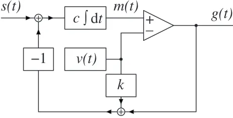
2. Mathematical formulation. In this section, we formulate a mathematical model for the design illustrated in Figure 1, which is arguably the simplest possible, chosen to illustrate most cleanly the dramatic effects of RC [12, 14].
For simplicity, the supply voltage has been scaled to±1; the input audio signal
s(t) lies in the range
−1< s(t)<1
for allt. Typically,s(t) contains audio in the range 20Hz–20kHz. The output g(t) is a high-frequency rectangular wave given by
g(t) =
1 fornT < t < An,
−1 forAn < t <(n+ 1)T,
whereT is the switching period, typically a few microseconds; for later convenience, we introduce the associated (angular) switching frequency
ωc =2π
+
+
d
t
+
_
m(t)
∫
g(t)
v(t)
−1
s(t)
k
c
Fig. 1.A first-order class-D amplifier with negative feedback and the option of RC. The input
audio signal iss(t). The output is a rectangular wave generated by a comparator (the triangular block): this wave isg(t) = sgn(m(t)−v(t)), where the carrier wavev(t)is a high-frequency sawtooth wave, and where m(t) is the time integral of the scaled error signal,c(s(t)−g(t)−kv(t)). k= 0 represents no RC;k= 1corresponds to RC.
A recipe will be given presently for calculating the modulated switching times An, the goal being that the low-frequency components ofg(t) should closely match s(t).
The rectangular wave g(t) is generated by comparing two signals and takes the values±1 according to which of those two signals is the greater. The first of these signals is a sawtoothcarrier wave, given by
(2.1) v(t) =−1 +2(t−nT)
T fornT < t <(n+ 1)T , v(t+T) =v(t).
The second signal,m(t), satisfies
(2.2) dm
dt =c(s(t)−g(t)−kv(t))
for some positive constantc, and is a continuous function of time, although its slope can be discontinuous at switching instants. The constant kindicates whether RC is applied (k= 1) or not (k= 0). This comparison process tells us that
g(t) =
1 whenm(t)> v(t),
−1 whenm(t)< v(t),
and we see that the switching times An are determined by the condition m(An) =
v(An). Hence, in view of (2.1), this switching condition amounts to
(2.3) m(An) =−1 + 2an,
where we have introduced the duty cyclesan, which are such that
(2.4) An= (n+an)T.
In view of the later need to integrate (2.2), we introducef(t) such that
[image:3.612.140.371.101.218.2]m(t)
n−1 An An+1
−1
+1
−1 +1
g(t)
t
(n−1)T nT
v(t)
A
m(t)
n−1 An+1
−1 +1
+3/2
−1/2
An
+1
−1
g(t)+v(t)
(n−1)T nT
g(t)
t v(t)
A
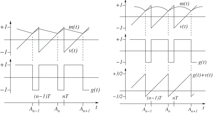
Fig. 2.Voltage waveforms without (left) and with (right) RC. In each case, for simplicity, the
input signals(t)has been shown as constant,s(t) = 12.
2.1. Ripple compensation. The nature of the input to the integrator depends significantly upon whether or not RC is applied.
Without RC, this input switches twice during each switching period: it is
(2.6) s(t)−g(t) =
s(t)−1 fornT < t < An,
s(t) + 1 forAn< t <(n+ 1)T,
which switches down by 2 at the (regularly spaced)unmodulated timest=nT and up by 2 at themodulatedtimest=An(which are not in general regularly spaced, as they depend ons(t)). In typical operation,s(t)−g(t) is nearly constant between switching instants, since the switching frequency is much greater than any audio frequencies.
One important source of distortion in the amplifier without RC arises because, as the duty cycle of the PWM signal varies, the shape of the comparator inputm(t) also varies. The slow modulation to the shape of m(t) gives rise to an unwanted, additional low-frequency input to the comparator, which generates output distortion. We quantify this aspect of the amplifier operation below.
With RC, by contrast, the integrator input switches only once in each switching period, since the regular up-switching ofg(t) and the regular down-switching ofv(t) at timest=nT cancel exactly: the integrator input is then
(2.7) s(t)−g(t)−v(t) =s(t)−2(t−nT)
T forAn−1< t < An.
This input switches up by 2 at times t=An and ramps downwards, nearly linearly, between switching instants. Now, crucially, the shape of the signal m(t) is almost the same between any two switching instants, regardless ofs(t); this feature of RC is responsible for its significant reduction of the output distortion.
[image:4.612.85.431.100.287.2]2.2. Further preliminaries. To avoid ambiguity, we record here the scalings that we adopt for the Fourier transform and its inverse, which will be used later:
ˆ
p(ω) =
∞
−∞
e−iωtp(t) dt, p(t) = 1 2π
∞
−∞
eiωtpˆ(ω) dω.
We also introduce the Diracδ-function, such that
∞
−∞
p(t)δ(t−t0) dt=p(t0)
wheneverp(t) is continuous att=t0.
3. Derivation of governing difference equations. In this section, we reduce the mathematical model given above in section 2 to a single, nonlinear difference equation for the duty cycle.
By successively integrating (2.2) over the time intervals An < t <(n+ 1)T and (n+ 1)T < t < An+1, using (2.6) and (2.7), we obtain
mn+1=m(An) +c(f((n+ 1)T)−f(An)) +c(k+ 1)(1−an)T −ck(1−a2n)T,
m(An+1) =mn+1+c(f(An+1)−f((n+ 1)T)) +c(k−1)an+1T−cka2n+1T,
where we have writtenmn+1 =m((n+ 1)T). If we next use the switching condition (2.3) to substitute form(An) andm(An+1) in these expressions and eliminatemn+1, we obtain a single difference equation for the duty cycle:
2(an+1−an) =c(f(An+1)−f(An))
+cT(1−(k+ 1)an+kan2 + (k−1)an+1−ka2n+1). (3.1)
This difference equation forms the basis of the analysis in the remainder of this paper. We note that, regardless of whether or not there is RC, (3.1) is inherently nonlinear for a time-varying audio input (sincef is then a nonlinear function). For more involved designs, the equivalent of (3.1) would be a vector difference equation (or, equivalently, a higher-order difference equation); cf. [13].
4. Behavior for constant input. In this section, we calculate the behavior of the device for a constant inputs(t)≡s0. This analysis provides the first clues to the effectiveness of RC in reducing audio distortion whens(t) is genuinely time-dependent. It also provides the basis for the small-signal model described in section 5.
We set s(t) = s0 and, correspondingly, from (2.5), f(t) = s0t. Substitution in (3.1) then gives the difference equation
2(an+1−an) =cT s0(1 +an+1−an)
+cT(1−(k+ 1)an+kan2 + (k−1)an+1−ka2n+1). (4.1)
This has the equilibrium solutionan =a, where
(4.2) a= 12(1 +s0),
irrespective of whether or not RC is applied. (This simple steady-state duty-cycle condition may alternatively be derived by noting that for a time-periodic response the mean input to the integrator over one cycle must be zero.) Linearization about the equilibrium point, withan =a+ Δan, gives
where
(4.3) α= 2−(1−k)cT s0.
Thus Δan =λnΔa0, withλ= (α−cT)/(α+cT). It follows that in the absence of RC the parameters must satisfy the condition
(4.4) 0< cT <2
in order to ensure stable operation for all s0. RC requires no such constraint for stability. Nevertheless, we assume that (4.4) holds in all that follows, so that com-parison can be made between the two cases. We note, furthermore, that without RC
λdepends ons0, but that with RCλis independent ofs0. This result gives the first hint that thedynamics of the system are significantly different in the two cases.
5. Small-signal model for perturbations to steady-state operation. Hav-ing calculated the steady-state response to a constant input, we next examine the dynamic response to small time-dependent input perturbations. Thus we suppose that
s(t) =s0+ Δs(t), f(t) =s0t+ Δf(t), g(t) =g0(t) + Δg(t), an=a+ Δan.
Here,ais given by (4.2) and we introduce the notation
(5.1) A¯n= (n+a)T.
In view of (2.5),
(5.2) Δs(t) = Δf(t).
Substituting these expressions in (3.1) and linearizing in perturbation quantities gives what engineers generally refer to as thesmall-signal model:
(5.3) (α+cT) Δan+1= (α−cT) Δan+cΔf( ¯An+1)−Δf( ¯An).
Recalling (4.3), we observe that with RC the coefficients in this small-signal model are independent ofs0; without RC, they are not.
To solve (5.3), we introduce an analytic functionxsuch that
(5.4) x( ¯An) = Δan.
Clearly (5.4) does not specifyxuniquely; we shall later choosexto have other con-venient properties. We then note that, by Taylor series,
Δan+1 =x( ¯An+1) =x( ¯An+T) = ∞
r=0
Tr
r! drx
dtr
t= ¯An
= eT Dx( ¯An),
whereD denotes the derivative operator d/dt. Thus (5.3) may be written [9] as
(5.5) (α+cT)eT D−(α−cT)x( ¯An) =c(eT D−1)Δf( ¯An).
perturbations to the output rectangular wave. We write the full outputg(t) as a sum of top-hat (or window) functions [4, 6]:
g(t) = ∞
n=−∞
ψ(t;nT, An)−ψ(t;An,(n+ 1)T),
where
ψ(t;t1, t2) =
1 fort1< t < t2, 0 otherwise.
It then follows that the output has Fourier transform (forω= 0)
(5.6) gˆ(ω) =
∞
−∞
e−iωtg(t) dt= 2(−iω)−1 ∞
n=−∞
e−iωAn−e−iωnT.
But the steady-state response has Fourier transform (again forω= 0)
ˆ
g0(ω) = 2(−iω)−1 ∞
n=−∞
e−iωA¯n−e−iωnT
and so, by taking the difference between these two results, we find
(5.7) Δˆg(ω) = 2(−iω)−1 ∞
n=−∞
e−iωA¯ne−iωT x( ¯An)−1.
Next we linearize (5.7): for any fixedω, we may replace
(5.8) e−iωT x( ¯An)−1→ −iωT x( ¯A
n),
leading to the linearized result that
(5.9) Δˆg(ω) = 2T ∞
n=−∞
e−iωA¯nx( ¯A
n).
The linearization in (5.8), which leads to (5.9), has a ready interpretation in the time domain, as we now describe. The output perturbation Δg(t) is in fact a train of narrow rectangular pulses: Δg(t) is generally zero, except for brief intervals between perturbed and unperturbed switching instants, during which it takes the values±2. Inverting the Fourier transform in (5.9) shows that the approximation (5.8) leads to
(5.10) Δg(t) =T
π
∞
n=−∞
x( ¯An)
∞
−∞
eiω(t−A¯n)dω= 2T
∞
n=−∞
x( ¯An)δ(t−A¯n),
We next use (5.9) to express Δˆgin terms of ˆx: first we note from (5.1) and (5.9) that
Δˆg(ω) = 2T ∞
−∞
e−iω(n+a)Tx((n+a)T) = 2T ∞
−∞
∞
−∞
e2πniτ−iω(τ+a)Tx((τ+a)T) dτ,
where the last step follows from Poisson resummation [10]. It then follows, upon making the substitutiont= (τ+a)T, that
(5.11) Δˆg(ω) = 2 ∞
−∞ e−2πnia
∞
−∞
e−i(ω−nωc)tx(t) dt= 2
∞
−∞
e−2πniaxˆ(ω−nωc).
The goal now is to use (5.5) to determine ˆx and then use (5.11) to derive the consequent perturbation to the output. In fact, we solve (5.5) under the more restric-tive condition that (5.5) holds at all times, not just the sample timest= ¯An. Then, replacing ¯An bytin (5.5) and taking the Fourier transform of the result, we have
(5.12) (α+cT)eiωT−(α−cT)xˆ(ω) =c(eiωT−1)Δ ˆf(ω).
To tidy the expressions below, we write (5.12) as
(α+cT)eiωT/2−(α−cT)e−iωT/2 xˆ(ω) =c(eiωT/2−e−iωT/2)Δ ˆf(ω).
Hence, using (5.2) we have
ˆ
x(ω) = tan
1 2ωT
ωT
1 + i α
cT tan12ωT
−1
Δˆs(ω)
and so, from (5.11),
(5.13) Δˆg(ω) = ∞
n=−∞
e−2πniaT(ω−nωc)Δˆs(ω−nωc),
whereT denotes thetransfer function
(5.14) T(ω) = 2 tan
1 2ωT
ωT
1 + i α
cT tan12ωT
−1
.
The transfer-function result in (5.13) and (5.14) is the culmination of the small-signal model.
There are two special cases of practical interest in which this result may be sim-plified, which we now examine in turn.
Single-frequency disturbance. The first case in which (5.13) may be simplified arises when the input disturbance is a single-frequency signal. Suppose Δs(t) =AeiΩt (subject to the constraint that Ω/ωc−12 is not an integer); then Δˆs(ω) = 2πAδ(ω−Ω). Note that the input frequency here is arbitrary (apart from the constraint noted): in particular, it need not be small compared to the switching frequency. Then, according to (5.13),
Δˆg(ω) = 2πA ∞
n=−∞
e−2πniaT(ω−nωc)δ(ω−nωc−Ω)
= 2πA T(Ω) ∞
n=−∞
Of particular interest is the response at the fundamental frequency. For ω near Ω, only the term forn= 0 is relevant and so to determine the fundamental response we have
Δˆg(ω)∼2πA T(Ω)δ(ω−Ω).
Thus the component of the output at the fundamental frequency is given by
Δg(t) =T(Ω)Δs(t).
Audio (low-frequency) disturbances. The second case concerns a distur-bance with all components in the audio band: specifically, we suppose that the dis-turbance to the input isband-limited, so that
Δˆs(ω) = 0 for|ω| ≥ωc/2.
Then, by virtue of (5.2) and (5.12), xis similarly band-limited. If we consider low-frequency components of the output (with |ω| < ωc/2), only the term n = 0 con-tributes to the sum in (5.13), and hence with these restrictions
(5.15) Δˆga(ω) =T(ω)Δˆs(ω),
where the subscript “a” indicates the audio (low-frequency) components of the output. Since audio frequencies are in practice much smaller than the switching frequency, we gain insight into the behavior of the amplifier by expanding T(ω) for small ω. Unfortunately, while (5.14) provides a compact representation of T(ω), it is not in a particularly convenient form for small-ω expansion. To provide a more fruitful expression, we write, from (5.2), (5.11), and (5.12),
(5.16) T(ω) = 2c(e
iωT −1)
(α−cT)iω(γeiωT −1), whereγ=
α+cT
α−cT.
Then it follows that
(5.17) T(ω) = 2cT
α−cT
∞
n=0
βn+2(1, γ)−βn+2(0, γ) (n+ 2)! (iωT)
n,
where theβn(ξ, γ) are the Apostol–Bernoulli functions, defined through the generating function [1]
(5.18) ze
ξz
γez−1 = ∞
n=0
βn(ξ, γ)
n! z
n.
We may simplify (5.17) using the identity [1]
(5.19) γβn(1, γ) =βn(0, γ)≡βn(γ) forn≥2,
to give
(5.20) T(ω) =−(γ−1)
2
γ
∞
n=0
βn+2(γ) (n+ 2)!(iωT)
Since [1]β2(γ) =−2γ/(γ−1)2,β3(γ) = 3γ(γ+ 1)/(γ−1)3,
β4(γ) =−4γ(γ
2+ 4γ+ 1)
(γ−1)4 , and β5(γ) =
5γ(γ3+ 11γ2+ 11γ+ 1) (γ−1)5 ,
it follows that for smallω,
T(ω)∼1− α 2ciω+
3α2−c2T2 12c2 (iω)
2+α(2c2T2−3α2)
24c3 (iω)
3.
Then inversion of the Fourier transform in (5.15) gives
Δga(t)∼Δs(t)− α 2cΔs
(t) +3α2−c2T2 12c2 Δs
(t)
+α(2c
2T2−3α2)
24c3 Δs (t). (5.21)
In practice, we expect terms in this series to diminish in size successively and the first few terms to provide a good approximation to the audio output. This follows because if Ω is a typical audio frequency, then parameters are generally chosen so that ΩT 1, whilecT = O(1); thenth derivative term in (5.21) is then O((ΩT)n/(cT)n), so terms on the right-hand side are of diminishing asymptotic size.
5.1. Reconstruction of the “full” output from the small-signal model. For the second of the cases above, we now show how the small-signal model may be extended to predict the amplifier output in response to a fully nonlinear input. In doing so, we highlight the particular influence of ripple compensation.
5.1.1. With RC. Since the coefficients in the expression (5.21) for the audio components of the output all become independent ofs0when RC is used, we deduce the followinglinear relationship in that case:
(5.22) ga(t)∼s(t)− α 2cs
(t) +3α2−c2T2 12c2 s
(t) +α(2c2T2−3α2) 24c3 s
(t),
even for signals that are not small.
In section 6, we shall directly calculate the output in response to a general audio input and show that the expression (5.22) provides an excellent approximation to the true audio output. It will turn out that in fact our deductions from the small-signal model, leading to (5.22), systematically omit terms that are nonlinear in time derivatives ofs(t) (such terms are removed by the linearization inherent in the small-signal model). We quantify these missing terms in section 6.
5.1.2. Without RC. Matters are more complicated without RC, since the transfer function depends on s0. However, we may still infer much about the au-dio output from the small-signal model. We have in (5.15) an expression that may be expanded in powers of iω in the form
(5.23) Δˆga(ω) = ∞
n=0
F
n(s0)(iω)nΔˆs(ω).
From (5.20), we see that the functionsFn satisfy
dFn ds0 =−
(γ−1)2
γ
βn+2(γ) (n+ 2)!T
If we now write
(5.24) Φn(γ) =Fn(s0),
then the chain rule gives
dΦn dγ =
dFn ds0
ds0 dγ =−
2βn+2(γ)Tn
γ(n+ 2)! =−
2βn+2(1, γ)Tn (n+ 2)! ,
where we have used (4.3) and (5.16), and where the last step uses the identity (5.19). Using the identity (A.3), which is derived in the appendix, we find
Φn(γ) =− 2βn+1(γ)T
n
(n+ 1)×(n+ 1)! + constant.
Fn(s0) is correspondingly obtained using (4.3), (5.16), and (5.24). We take one of the constants of integration so thatF0(0) = 0; the other constants are immaterial in view of the time derivatives taken below, in (5.25).
We may now reconstruct the full audio output ga(t), as predicted by the small-signal model. By inverting the Fourier transform in (5.23), it follows that
Δga(t) = ∞
n=0
F
n(s0)DnΔs(t).
But
DnF
n(s(t)) =DnFn(s0+ Δs(t))∼Fn(s0)DnΔs(t),
where the last step follows from repeated application of the chain rule and lineariza-tion. Thus we infer from the small-signal model that the audio output is (omitting terms that are nonlinear in time derivatives, and hence invisible to the small-signal analysis)
ga(t) =s(t) + ∞
n=1
dn
dtnFn(s(t)) (5.25)
=s(t)−2 ∞
n=1
Tn
(n+ 1)×(n+ 1)! dn
dtnβn+1(Γ(t)),
where
Γ(t) = 2 +cT(1−s(t)) 2−cT(1 +s(t)).
Hence the small-signal analysis predicts the followingnonlinear audio output:
ga(t)∼s(t) +
−s(ct)+T s
2(t)
4
+
s
(t)
c2 −
T2s(t)
12 −
T s2(t)
2c +
T2s3(t)
12
.
6. Fully nonlinear audio output. Our mathematical analysis has so far con-cerned an input signal that is a constant plus an infinitesimal time-dependent pertur-bation. In this section, we instead calculate the fully nonlinear response to a general time-varying input signals(t). This calculation will corroborate the small-signal re-sults and will complete that analysis by providing the missing terms. The calculation of this section is a perturbation calculation based on the assumption that the audio signal varies slowly compared to the switching (which is generally the case).
6.1. Perturbation framework. We suppose now that the audio input s(t) is time-varying, with a typical (angular) frequency Ω (we emphasize that there is no assumption that the input is sinusoidal, merely that Ω is representative of the audio frequencies present). We introduce the small parameter
≡ΩT 1
and construct a perturbation solution for the audio output of the amplifier, following our earlier treatments of other class-D designs [4, 5, 6].
To emphasize the time scales of the various quantities involved in the analysis, we introduce a dimensionless time variable
(6.1) σ= Ωt=t/T
and write
s(t) =S(σ), f(t) =T
F(σ),
and hence, given (2.5), S(σ) = F(σ). We now introduce A(σ) such that sampled values are specified by
(6.2) A(n) =an.
The governing equation for A is then the exact difference equation (3.1), which be-comes, in the present notation, either with or without RC,
2(A(n+)− A(n)) = cT
F(n++A(n+))− F(n+A(n))
+cT1−(k+ 1)A(n) +kA2(n)
+ (k−1)A(n+)−kA2(n+). (6.3)
We note that the discrete equation (6.3) holds for integer n. To make analytical headway, we seek a particular solution that also satisfies the corresponding equation at intermediate points. Thus we seek a solution to
2(A(σ+)− A(σ)) = cT
(F(σ++A(σ+))− F(σ+A(σ)))
+cT1−(k+ 1)A(σ) +kA2(σ)
+ (k−1)A(σ+)−kA2(σ+). (6.4)
Since we have been unable to find a general solution to this equation for A(σ), we instead attempt to solve for successive terms in the perturbation series
by solving (6.4) at successive orders in. Using computer algebra to accomplish the details, we find the first couple of results to be
A0(σ) = 12(1 +S(σ)), A1(σ) =
1 4 −
1 2cT
S(σ) +2−k 4 S(σ)S
(σ);
the first is an analogue of the steady-state duty-cycle result (4.2). However, results forA(σ) are in themselves rather unedifying. To see their practical import, we next calculate the corresponding audio components of the outputg(t).
We now apply Poisson resummation to the Fourier transform of the full output and adopt the notation in (6.2) to give
ˆ
g(ω) = 2
−iω ∞
n=−∞
∞
−∞
e2πniτe−iωτT(e−iωA(τ)T −1) dτ
= 2
−iωT ∞
n=−∞
∞
−∞
e−i(ω−nωc)t(e−iωA(t/T)T −1) dt.
(6.6)
Now we focus on the audio components of the output, specifically with|ω| < ωc/2; we make the reasonable assumption that these are dominated by the termn= 0 in (6.6). After Taylor-expanding the exponential involvingA(t/T) in (6.6), we have
ˆ
ga(ω) = 2
∞
−∞ e−iωt
∞
n=0
(−T)n (n+ 1)!
dn dtnA
n+1(t/T) dt,
where we have used the result that the Fourier transform ofp(t) is iωpˆ(ω). Hence, by inverting the Fourier transform, we obtain
ga(t) = constant + 2 ∞
n=0
(−T)n (n+ 1)!
dn dtnA
n+1(t/T),
where the constant is not determined by the analysis above (in view of the restriction to ω = 0 in expressions such as (6.6)). This constant may readily be obtained by noting thatg(t) =−1 for allt whenA(σ) = 0 for allσ; hence
ga(t) =−1 + 2 ∞
n=0
(−T)n (n+ 1)!
dnAn+1(t/T) dtn
=−1 + 2 ∞
n=0
(−)n (n+ 1)!
dnAn+1(σ) dσn . (6.7)
6.2. Results with and without RC. We find, after substituting our solution forA(σ) in (6.7) and reverting to the original notation of the problem, that the audio component of the output satisfies
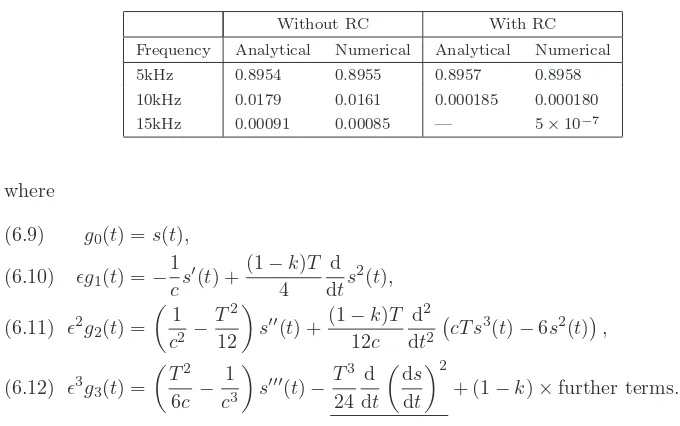
Table 1
Results for s(t) = 0.9 sin 2πf1t, with f1 = 5kHz, giving the amplitudes of the fundamental,
second, and third harmonics in the output. The missing entry indicates that, to the order we have calculated, our analytical results predict only second-harmonic distortion with RC (although higher harmonics arise later in the perturbation expansion of the output).
Without RC With RC
Frequency Analytical Numerical Analytical Numerical
5kHz 0.8954 0.8955 0.8957 0.8958
10kHz 0.0179 0.0161 0.000185 0.000180 15kHz 0.00091 0.00085 — 5×10⁻⁷
where
g0(t) =s(t), (6.9)
g1(t) =−1
cs(t) +
(1−k)T 4
d dts
2(t),
(6.10)
2g 2(t) =
1
c2 −
T2
12
s(t) +(1−k)T 12c
d2 dt2
cT s3(t)−6s2(t),
(6.11)
3g 3(t) =
T2
6c − 1
c3
s(t)−T3 24
d dt
ds dt
2
+ (1−k)×further terms. (6.12)
We see now that without RC (i.e., takingk= 0), nonlinearity insarises in each term fromg1 onwards. This nonlinearity causes (undesirable) harmonic distortion in the output. Furthermore, we note that all contributions ing0,g1, andg2are predicted by our analysis of the small-signal model (cf. (5.26)), although the underlined term in
g3 cannot be found from that model, because it involves products of time derivatives (neither can some of the other terms in the mess we have denoted “further terms”).
The significant benefit of RC (with k= 1) appears starkly in the results above: all terms in the full audio output are linear ins, untilO(3), where the first nonlinear term occurs. Recall that the output predicted by the small-signal model in this case is entirely linear ins, so any nonlinearity in the full output is beyond that model.
6.2.1. Simulation results. To corroborate the analysis above, we have carried out simulations of the amplifier with and without RC, using (3.1) to calculate a sequence of output switching times. We then discard initial transients and use (5.6) to determine the corresponding output Fourier transform ˆg(ω) (with slight modifications because our simulation has finite duration). We are thus able to determine numerically the contributions to the output at various frequencies. We then compare these to the asymptotic predictions from (6.8)–(6.12). The amplifier parameters are chosen to be typical for the operation of this device: T−1= 384kHz andc= 0.8/T.
We carry out two sets of simulations: in the first, s(t) = 0.9 sin 2πf1t, with
f1 = 5kHz, and we expect to see this fundamental and its harmonics in the output; in the second, s(t) = 0.5 sin 2πf0t+ 0.4 sin 2πf1t, with f0 = 1kHz and f1 = 5kHz, and we expect to see in addition “intermodulation terms” with frequencies that are integer combinations of f0 andf1. If we choose the “typical” frequency as 5kHz in each case, then our small parameter is= 2πf1T ≈0.08.
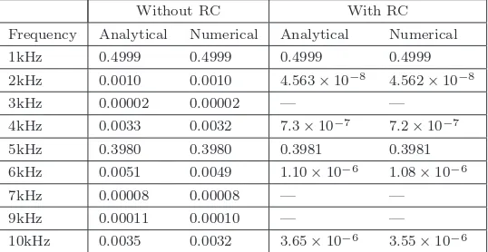
Table 2
Results for s(t) = 0.5 sin 2πf0t+ 0.4 sin 2πf1t, with f0 = 1kHz and f1 = 5kHz, giving the
amplitudes of the output contributions at various frequencies. Missing entries indicate either terms absent from the analytical expression for the output to the order calculated or negligible numerical contributions.
Without RC With RC
Frequency Analytical Numerical Analytical Numerical
1kHz 0.4999 0.4999 0.4999 0.4999
2kHz 0.0010 0.0010 4.563×10⁻⁸ 4.562×10⁻⁸
3kHz 0.00002 0.00002 — —
4kHz 0.0033 0.0032 7.3×10⁻⁷ 7.2×10⁻⁷
5kHz 0.3980 0.3980 0.3981 0.3981
6kHz 0.0051 0.0049 1.10×10⁻⁶ 1.08×10⁻⁶
7kHz 0.00008 0.00008 — —
9kHz 0.00011 0.00010 — —
10kHz 0.0035 0.0032 3.65×10⁻⁶ 3.55×10⁻⁶
those not quoted explicitly in (6.12) (although we note that the terms ing3affect only the fourth decimal place of the analytical result). With RC, the harmonics are much smaller than without; said differently, there is less harmonic distortion. Again, we use terms up to and including g3 for the analytical results; the only nonlinear term is then that underlined in (6.12), so there is not yet any third or higher harmonic present in the analytical result.
Results for the second simulation are summarized in Table 2, where we have included the main output frequency components in the range 1–10kHz. This provides a more exacting test of the nonlinear terms than does the first simulation. Both with and without RC, there is excellent agreement between analysis and numerics. Since the analytical results include terms up to g3, with RC the only nonlinearity is quadratic and hence the only frequency components generated in the range 1– 10kHz are those with nonzero entries in Table 2. The impressive performance of RC in removing extraneous frequency components from the output is clear (that is, RC significantly reduces the so-called intermodulation distortion).
7. Conclusions. Ripple compensation (RC) [12, 14] is a highly effective means of significantly reducing audio distortion in class-D amplifiers. Through achieving the highest possible loop gain across the audio band, the technique is able to suppress imperfections in the output stage. RC may also be used to improve the performance of other switching technologies, such as current and voltage control loops, DC-to-DC or DC-to-AC power converters, or high-precision motor drives. In this paper, we have presented the first detailed mathematical analysis of this technique, leading to an explicit expression for the fully nonlinear audio output of the amplifier. This expres-sion quantifies in detail for the first time how RC significantly linearizes the amplifier output and thus fundamentally improves our understanding of the RC technique.
Our work has proceeded by first reducing the mathematical model to a nonlinear difference equation for the duty cycle. This approach effectively “factors out” the fast dynamics associated with the switching and can be applied generally to switching systems. Of course, the idea of such a reduction to difference equations is clearly not new (see, for example, [13, 16]), but in the literature the subsequent analysis usually focuses on determination of the steady-state operating point and investigation of its stability and bifurcations as the parameters of the problem are varied. By contrast, here our interest is in the response to slowly varying input, under the assumption of stable operation.
We close by noting that one aspect of particular significance in the present work is our extension of the standard small-signal model to yield the most significant com-ponents of the audio output in response to ageneral audio input signal. This aspect of our work has wide potential applicability beyond the present case.
Appendix. An identity for Apostol–Bernoulli functions. Consider Θ(z, γ) = ln|γez−1|. By differentiation,
(A.1) ∂Θ
∂z =γ ∂Θ
∂γ =
γez
γez−1 =γ ∞
n=1
βn(1, γ)
n! z
n−1,
where we have used (5.18). Integrating∂Θ/∂zwith respect to zthen gives
(A.2) Θ(z, γ) = ln|γ−1|+z+ ∞
n=1
βn(γ)
n×n!z
n,
where we have used (5.19). Then substituting (A.2) in∂Θ/∂γ in (A.1) gives
1
γ−1+ ∞
n=1
β
n(γ)
n×n!z
n=∞
n=0
βn+1(1, γ) (n+ 1)! z
n.
By equating powers ofz in this expression, we see thatβ1(1, γ) = 1/(γ−1) and that
(A.3) βn(γ) = nβn+1(1, γ)
n+ 1 forn= 1,2, . . ..
REFERENCES
[1] T. M. Apostol,On the Lerch zeta function, Pacific J. Math., 1 (1951), pp. 161–167.
[2] M. Berkhout and L. Dooper,Class-D audio amplifiers in mobile applications, IEEE Trans.
Circuits Syst. I. Regul. Pap., 57 (2010), pp. 992–1002. [3] H. S. Black,Modulation Theory, Van Nostrand, New York, 1953.
[4] S. M. Cox and B. H. Candy,Class-D audio amplifiers with negative feedback, SIAM J. Appl.
Math., 66 (2005), pp. 468–488.
[5] S. M. Cox, C. K. Lam, and M. T. Tan,A second-order PWM-in/PWM-out class-D audio
amplifier, IMA J. Appl. Math., 78 (2013), pp. 159–180.
[6] S. M. Cox, M. T. Tan, and J. Yu,A second-order class-D audio amplifier, SIAM J. Appl.
Math., 71 (2011), pp. 270–287.
[7] R. W. Erickson and D. Maksimovi´c,Fundamentals of Power Electronics, 2nd ed., Springer,
New York, 2001.
[8] D. G. Holmes and T. A. Lipo,Pulse Width Modulation for Power Converters, IEEE Press,
Piscataway, NJ, 2003.
[9] L. M. Milne-Thomson,The Calculus of Finite Differences, Macmillan, London, 1933.
[10] P. M. Morse and H. Feshbach,Methods of Theoretical Physics, Part I, McGraw–Hill, New
[11] T. Mouton, A. de Beer, B. Putzeys, and B. McGrath,Modelling and design of single-edge
oversampled PWM current regulators usingz-domain methods, in ECCE Asia Downunder (ECCE Asia), IEEE, Piscataway, NJ, 2013, pp. 31–37.
[12] T. Mouton and B. Putzeys,Digital control of a PWM switching amplifier with global
feed-back, in Audio Engineering Society Conference: 37th International Conference: Class D Audio Amplification, Audio Engineering Society, 2009.
[13] G. A. Papafotiou and N. I. Margaris,Calculation and stability investigation of periodic
steady states of the voltage controlled buck DC–DC converter, IEEE Trans. Power Elec-tronics, 19 (2004), pp. 959–970.
[14] B. Putzeys,Simple, ultralow distortion digital pulse width modulator, in Audio Engineering
Society Convention: 120th Convention: Paris, France, Audio Engineering Society, 2006. [15] L. Risbo and C. Neesgaard,PWM amplifier control loops with minimum aliasing
distor-tion, in Audio Engineering Society Convention: 120th Convention: Paris, France, Audio Engineering Society, 2006.
[16] C. K. Tse and M. di Bernardo,Complex behavior in switching power converters, Proc. IEEE,