A quantitative systems pharmacology approach, incorporating a novel liver model, for predicting pharmacokinetic drug drug interactions

A quantitative systems pharmacology

approach, incorporating a novel liver model,

for predicting pharmacokinetic drug-drug

interactions

Mohammed H. Cherkaoui-Rbati1*, Stuart W. Paine1, Peter Littlewood2, Cyril Rauch1

1 School of Veterinary Medicine and Science, University of Nottingham, Sutton Bonington, Leicestershire, United Kingdom, 2 Vertex Pharmaceuticals (Europe) Limited, Abingdon, Oxfordshire, United Kingdom

*mohammed.h.cherkaoui@gmail.com

Abstract

All pharmaceutical companies are required to assess pharmacokinetic drug-drug interac-tions (DDIs) of new chemical entities (NCEs) and mathematical prediction helps to select the best NCE candidate with regard to adverse effects resulting from a DDI before any costly clinical studies. Most current models assume that the liver is a homogeneous organ where the majority of the metabolism occurs. However, the circulatory system of the liver has a complex hierarchical geometry which distributes xenobiotics throughout the organ. Never-theless, the lobule (liver unit), located at the end of each branch, is composed of many sinusoids where the blood flow can vary and therefore creates heterogeneity (e.g. drug con-centration, enzyme level). A liver model was constructed by describing the geometry of a lobule, where the blood velocity increases toward the central vein, and by modeling the exchange mechanisms between the blood and hepatocytes. Moreover, the three major DDI mechanisms of metabolic enzymes; competitive inhibition, mechanism based inhibition and induction, were accounted for with an undefined number of drugs and/or enzymes. The liver model was incorporated into a physiological-based pharmacokinetic (PBPK) model and sim-ulations produced, that in turn were compared to ten clinical results. The liver model gener-ated a hierarchy of 5 sinusoidal levels and estimgener-ated a blood volume of 283 mL and a cell density of 193×106cells/g in the liver. The overall PBPK model predicted the pharmacoki-netics of midazolam and the magnitude of the clinical DDI with perpetrator drug(s) including spatial and temporal enzyme levels changes. The model presented herein may reduce costs and the use of laboratory animals and give the opportunity to explore different clinical scenarios, which reduce the risk of adverse events, prior to costly human clinical studies.

Introduction

A pharmacokinetic drug-drug interaction (DDI) is where a drug(s), the perpetrator drug(s), interacts with a metabolizing enzyme(s) or membrane transporter(s) such that the

a1111111111 a1111111111 a1111111111 a1111111111 a1111111111

OPEN ACCESS

Citation: Cherkaoui-Rbati MH, Paine SW,

Littlewood P, Rauch C (2017) A quantitative systems pharmacology approach, incorporating a novel liver model, for predicting pharmacokinetic drug-drug interactions. PLoS ONE 12(9): e0183794.https://doi.org/10.1371/journal. pone.0183794

Editor: Jinn-Moon Yang, National Chiao Tung

University College of Biological Science and Technology, TAIWAN

Received: November 30, 2016

Accepted: August 11, 2017

Published: September 14, 2017

Copyright:©2017 Cherkaoui-Rbati et al. This is an open access article distributed under the terms of theCreative Commons Attribution License, which permits unrestricted use, distribution, and reproduction in any medium, provided the original author and source are credited.

Data Availability Statement: All relevant data are

within the paper and its Supporting Information files.

Funding: The funder, Vertex Pharmaceutical,

pharmacokinetics (PK) of another drug(s), the victim drug(s), is altered. In the late 1970s, the first cases of pharmacokinetic DDIs were reported [1], and since then more and more DDIs have been identified especially in the situation of polypharmacy as is often the case for elderly patients [2]. The increase in observed DDIs coupled to some lethal cases [1] led the FDA to publish in 1997 the firstin vitrometabolism drug interaction guidance document [3] for phar-maceutical companies. In order to identify the possible interactions of new chemical entities (NCEs), many strategies have been suggested as it is essential to know before costly clinical tri-als, whether a NCE will be a safe drug. One of those strategies relies on the combination ofin vitroinformation coupled to mathematical models to predict the clinical DDIs. This has the advantage to be cost effective, reduce the use of laboratory animals and give the opportunity to explore different clinical scenarios in order to identify optimum dose regimens. Excluding the limitations ofin vitroexperiments, the modeling approach is limited by the sophistication of the implemented models. Current models are classified into two different categories that depend on whether they are a function of time or not (i.e. static and dynamic models), and mainly focus on one enzyme and/or one particular aspect of DDIs (e.g. reversible inhibition [4], mechanism based inhibition [5] or induction [6]). In their most advanced form the static models may account for all kinds of DDIs [7], but are limited in their ability to describe com-plex mechanisms related to administration, distribution, metabolism or excretion such as active drug transport (uptake) into hepatocytes or enterocytes. Although the dynamic models are more descriptive, traditionally, the dynamic models were developed to describe specific drug cases [4,5,8] and most of them assume that the liver is a homogeneous organ (e.g. well-stirred model [9,10]) where the majority of the metabolism occurs. However, the circulatory system of the liver has a complex hierarchical geometry which helps to distribute xenobiotics throughout the organ. Nevertheless, the lobule (liver unit), located at the end of each branch, is composed of many sinusoids (small blood vessels) where the blood flow can vary and therefore creates heterogeneity (e.g. drug concentration, enzyme level). Some liver models account for heterogeneity, such as the parallel tube model [9,10] and the dispersion model [11,12], but they have not been used to predict DDIs and do not account for the variation in blood flow through the lobules. With established methodologies ofin vitroscreening for DDIs, pharma-ceutical companies need adequate tools to predict the net result ofin vivoDDIs to translate theirin vitroobservations to clinical predictions. It is common for elderly patients to receive several medications to treat different symptoms or conditions. Each of these medicines can potentially interfere with the usual routes of metabolism for another drug. There is a serious need for better models to cover all different scenarios, which also takes into account the vari-abilities between individuals, such as size, weight and differences in genetic polymorphisms [13]. In this paper, a liver model will be presented that takes into account three major DDI mechanisms of metabolic enzymes; competitive inhibition, mechanism based inhibition (MBI) and induction, with an undefined number of drugs and/or enzymes, where the lobule geometry will be accounted for due to its impact on blood flow heterogeneity. The liver model will then be incorporated into a physiological-based pharmacokinetic (PBPK) model and sim-ulations produced that in turn will be compared to clinical results. The description of the model proposed herein is divided into six parts. The first part will introduce the model and the notations used throughout the document including a new liver model taking into consider-ation its hierarchical structure and the different body compartments that are essential to drug metabolism. In the second part, the algorithm to generate the lobule geometry will be pre-sented, where length and radius of the sinusoids are produced. In the third part, the transport and metabolism reactions of the drugs will be mathematically described. As the drugs are dis-tributed in the body through the bloodstream, the conservation equation will be used in the liver sinusoids to describe the blood transport and the exchange mechanisms between the University of Nottingham from the

conceptualization to the validation of the PhD. Finally he was also part of the review of this manuscript. This does not alter our adherence to PLOS ONE policies on sharing data and materials.

Competing interests: There are no patents,

blood and hepatocytes, such as passive diffusion and active uptake/efflux of the drugs. Inside the hepatocytes, drug metabolism and drug interactions with metabolic enzymes will be described. In the fourth part, the PBPK model presented in part one will be fully developed. In part five, a brief description on how the PBPK was numerically resolved will be given. In the sixth part, drugs for which data exist will be considered and their physiological parameters defined. Finally the results from the new liver model will be presented and compared to clinical data.

Models

Presentation of the liver model and notations

The objective of this section is to provide a brief explanation of the subsequent models that will be used to develop a formal understanding of DDIs. There are three major aspects to con-sider; (i) the geometry of the lobule (ii) the set of complex interactions between xenobiotics and enzymes (iii) the usual set of body compartments (PBPK Model).

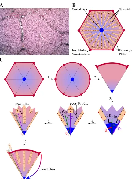
Drugs move with the flow of blood and as a result the exchange mechanisms of drug between the blood and the tissue will be a function of the lobule geometry in which the flow takes place. The lobules have a peculiar shape idealized as hexagons composed of a series of peripheral entries (portal veins and hepatic arteries) and a central vein (Fig 1A and 1B). This spatial configuration and its hierarchical structure will need to be taken into consideration in order to describe the blood flow and to generate an algorithm to construct a lobule within the physiological constraints. Furthermore, the blood velocity will be assumed constant and aver-aged over the cross section of sinusoids present within the lobule while it will vary along the length of sinusoids as their radii narrow. The latter assumption is the only one that will be used, which reduces the spatial dimension to one. The spatial variable is notedxand for each sinusoids portion thex-axis is taken along the bisector and goes from the external part of the lobule to the central vein (Fig 1C).

To describe the DDIs no assumptions will be made on the number of drugs and enzymes involved to make the model generic for all animal species. However, the only way to achieve this is to consider matrix calculus. While this may appear as an unnecessary complication at first sight, it will be seen that with adequately defined operators the writing of equations is largely intuitive even for those not fully familiar with matrix algebra. To start with, the follow-ing notationsnCandnEwill refer to the number of drugs and enzymes, respectively. To distin-guish between scalars and matrices (including vectors), matrices and vectors are written in bold. Thus any set of variables or constants related to drugs shall be described as a column vec-tor of sizenCincluding their concentrations:C = (C1 CnC)

tr_{or membrane permeability:}

P = (P1 PnC) tr

. Note here that the subscript “tr” refers to the transposition of a column vector into a vector line (the same notation shall be used for matrices where in this case the operator transposed is noted:Atr_{¼ ða}tr

i;jÞ1im

1jn

¼ ðaj;iÞ1im

1jn

whereA¼ ðai;jÞ1in

1jm

). Similarly, any

set of variables or constants related to enzymes or their degradation shall be described as a col-umn vector of sizenEincluding for example the enzyme concentrations:E = (E1 EnE)

tr_{; or}

their degradation:kdeg= (kdeg, 1 kdeg,nE)

tr_{. As the number of possible pair interactions}

between enzymes and drugs is given by the scalar product:nC×nE, one defines the matrix EC¼ ðECi;jÞ1inC

1jnE

where the termECi,jrepresents the interaction of thei-th drug with the

define the reaction rate of the reaction. To use matrices one needs to define the following oper-ators: “” such thatkcatEC¼ ðkcat;i;jECi;jÞ1inC

1jnE

. By extension, a division operator is

defined and noted “/” or “−” between vectors or matrices such that: x=y¼x y¼

xi;j

yi;j 1in

1jm .

Finally for completion the column vectors of sizenCornEand of components equal to unity shall be noted:1_n

Cand1nE.

Last but not least, a seven-compartment model is used involving: venous blood, arterial blood, liver, gut, kidneys, lungs (to consider the pulmonary circulation), and the rest of the body (Fig 2). The average volume and blood flow of each compartment is given inS1 Table.

Lobule geometry

The lobule is the elementary unit of the liver where the exchange of nutrients and xenobiotic compounds occurs between the blood and the hepatocytes. The shape of the lobule and the spatial distribution of the hepatocytes are irregular in appearance (Fig 1A). But schematically, the liver lobule can be represented by a hexagon (Fig 1B), where the hepatic vein is at the cen-tre and where at each apex, the hepatic artery and the hepatic portal vein pour blood into the sinusoids. The sinusoids are converging toward the centre where the blood leaves the lobule through the central vein (Fig 1B).

To suggest a theory on which an amenable model will be based, the lobule geometry will be simplified. The parameters used to define the geometry are summarized inTable 1, whereas the algorithm to build the lobule geometry for the simulations is schematically represented in Fig 1Cwhere each step is numbered and detailed as below:

1. The hexagonal shape of the lobule is replaced by a disc of similar area:3pffiffi3

2 R

2

lobule¼pR

2

Circle.

2. Due to the symmetry of an hexagon, only one sixth of the circle will be taken into account.

3. The initial two hepatocyte plates are placed on either edge of the sector (one sixth of the cir-cle) and respect a minimal distance of 2RSinbetween the hepatocytes plates, the initial dis-tances from the centre are estimated by:

a. The first sinusoid output:x0¼ _tanRSin_y 1þ

e

2siny1

whereyk¼ y0

2kandθ0= 60˚.

b. The first hepatocyte plate:y0¼ _sinRSin_y 1

þ e

2tany1.

c. Iteration initialization:k= 0

4. A loop is implemented as follow: whilexkRCircledo

a. k=k+ 1

b. Place a hepatocyte plate on each line of angleθk+ (i− 1)θk− 1for8i2{1,. . ., 2k− 1},

such as the minimal distance of the new hepatocyte plate to the previous one is 2RSincos

θk+ 1, which gives an output diameter of 2RSin.

c. The distance of the outputs:xk¼ _tanRSin_y

kþ1þ

e

2_sinykþ1.

automatically generate the length and radius of the sinusoids. The latter is used to estimate the changes in velocity within a sinusoid portion by assuming a constant blood flow and a constant velocity over the cross section.

Fig 2. The seven compartmental model. Red and blue arrows represent blood flows (Qiwhere i represents: T for total blood flow, ha

hepatic artery blood flow, pv portal vein blood flow, L for the liver blood flow, G for the gut blood flow, K for the kidneys blood flow and RB for the blood flow going to the rest of the body). The black arrows represent absorption (ka: absorption constant rate) or excretion (CLR: Renal

Clearance).

d. The distance of the new plates:yk¼ _sinRSin_y

kþ1

þ e

2tanykþ1.

5. WhenxkRCirclethe last level of sinusoid is reached and one posesn=k. Then in order to

be consistent with the direction of the blood flow, the level 1 is defined as the furthest level from the central vein, and the levelnas the closest one.

6. As a result, the length of each sinusoids level is given by:Lk= min(yn−k+1,RCircle)−xn−k.

Now that the number and the length of the sinusoid levels are defined, the radius within each level changes which is expected to impact the exchange of chemicals between the blood and the hepatocytes. Therefore it is essential to calculate the sinusoid radius changes for every level defined above. The radius along the sinusoids of levelk, following the blood flow, is then given by:

RkðxÞ ¼RSinþ ðLk xÞtanyn kþ1 8x2 ½0 :LkŠ ð1Þ

Finally, as one assumes that the blood flowQkat a given levelkis identical for all sinusoids, the blood flow and the average velocity are given by:

Qk ¼

QLobule

62n k

vkðxÞ ¼

Qk

pRkðxÞ

28x2 ½0 :LkŠ

8 > > <

> > :

ð2Þ

where the flow in a lobule isQLobule=QLiver/NLobulewithNLobule=VLiver/VLobuleandVLiverand

VLobuleare, respectively, the liver and lobule volumes. This assumes the same flow in each lob-ule. Finally, to simplify the notation, in the remaining text we define:

8x2 ½0 :L_nŠ

RðxÞ ¼R1ðxÞ1½L0:L1Šþ

Xn

k¼2

Rkðx Lk 1ÞIŠLk 1:LkŠðxÞ

QðxÞ ¼Q1ðxÞ1½L0:L1Šþ

Xn

k¼2

Qkðx Lk 1ÞIŠL_k1:LkŠðxÞ

vðxÞ ¼v1ðxÞ1½L0:L1Šþ

Xn

k¼2

vkðx Lk 1ÞIŠLk1:LkŠðxÞ

8 > > > > > > > > > > > <

> > > > > > > > > > > :

ð3Þ

where8k2〚1: n〛Lk ¼Lk 1þLk,L0 ¼0andIEis the indicator function ofE.

Table 1. Lobule parameters.

Parameter Description Value

RLobule Lobule Radius 790.57μm [14]

Rsin Minimal Sinusoidal Radius 3.65μm [14]

eLobule Lobule Thickness 25.00μm [14]

RH Hepatocyte Radius 8.49μm [14]

e Hepatocyte Plate Width(= 2RH) 16.97μm

Conservation and kinetic equations for the liver model

Conservation equation in the blood. Now that the lobule geometry has been defined, the

equations which describe the transport and metabolism of drugs in the liver can be expressed. Before being metabolized in the hepatocytes, the drugs flow with the blood through the lobules and are passively or actively transported into the hepatocytes. ConsideringnCdrugs and assuming no irreversible reaction within the blood, the conservation equation can be used to describe the concentrations such as:

@Cb @t þv xð Þ

@Cb

@x ¼ aB!Hð Þx ðPþρinÞ f b

uCb ðPþρoutÞ f h uCh

ð4Þ

whereCb,Ch,P, ρin,ρout,fbu,f h

uandv(x) are, respectively, the concentrations of the drugs in the liver blood and hepatocytes, the permeability and the uptake/efflux rates through the hepatocyte membrane, the fraction unbound in the blood and hepatocytes and the blood velocity; and whereαB!H(x) is the ratio of the elementary blood-hepatocyte surface exchange

δSExchange(x) to the elementary blood volumeδVBlood(x) (seeS1 Appendix), given by:

a_B!Hð Þ ¼x

2R xð Þ þeL 2RH

cosyðxÞ RðxÞðeL 2RHÞ

ð5Þ

As the blood flow enters the sinusoid from the hepatic arteries atx= 0, the initial and bound-ary conditions are given by:

Cbðx>0;t¼0Þ ¼0

C_bðx¼0;tÞ ¼C0ðtÞ

Chðx;t¼0Þ ¼0

8 > <

>

: ð6Þ

whereC0(t) will be defined once the PBPK model will be decribed.

Drug kinetic equation in the hepatocytes. Once the drugs enter inside the hepatocytes

by passive and/or active transport, a cascade of reactions may occur involving metabolism of the drugs by one or more enzymes and includes cross reaction(s) between metabolite(s) and drug(s). The presented model focuses specifically on the reactions schematically represented inFig 3(i.e. Competitive Inhibition, MBI and Induction).

Furthermore, it will be assumed that no exchange of materials between hepatocytes happens and that the equilibrium between the drugs and enzyme complex is quickly reached (seeS2 Appendixfor the mathematical simplification). Therefore, by using the law of conservation of mass, one can describe the equation governing the concentration of drugs within the hepato-cytes by:

dCh

dt ¼ aH!BðxÞ½ðPþρinÞ f b

uCb ðPþρoutÞ f h uChŠ

ðkcatECMetÞ1n_E

ðkinactECMBIÞ1nE

Vmax;2 Km;2þf

h uCh

fhuCh

ð7Þ

whereECMet¼ ðECMet;i;jÞ1inC

1jnE

metabolism of drugs,EC_MBI ¼ ðEC_MBI;i;jÞ1inC

1jnE

the concentration of complex inactivating the

enzymes and;Vmax, 2andKm, 2the constants associated with unspecified metabolic pathway (s), modeled by a Michaelis-Menten equation. FinallyαH!B(x) is the ratio of the elementary blood-hepatocyte surface exchangeδSExchange(x) to the elementary hepatocyte volumeδVHep(x) (seeS1 Appendix), given by:

a_H!Bð Þ ¼x

2R xð Þ þeL 2RH cosy

RH 2Rkð Þ þx

eL cosy

ð8Þ

Eq (7)can be rewritten considering the rapidly attained equilibrium assumption. In this context the enzyme-drug complex concentrations can be expressed as a function of the free

Fig 3. Enzymatic reactions taken into account in the liver model. Reversible inhibition: A drug binds to an enzyme which may result in its metabolism (but not necessarily) resulting in the temporary blockade or inhibition of the enzyme. Here only competitive inhibition will be studied, which assumes that each enzyme can interact with one drug at a time. Mechanism Based Inhibition (MBI): A drug inactivates an enzyme through direct interaction resulting in an inhibited metabolism of any drug metabolized by these enzymes. Induction: A drug induces the expression of one or more enzymes resulting in an induced metabolism of any drug metabolized by these enzymes. Note that the notations in this figure regarding the kinetic rate constants are used in the text.

enzyme levels and drug concentrations as follow:

ECMet¼

ðfhuChÞE tr

Km;1

ECMBI¼

ðfh_uChÞE

tr

KI

ð9Þ

whereE = (E1,. . .,EnE)

tr_{represents the free enzyme levels and where the constants}

Km;1¼

k21þkcat k12

andKI¼

k41þkinact k14

are developed inS2 Appendix. Therefore the equation

becomes:

dCh

dt ¼ aHBðxÞ½ðPþρinÞ f b

uCb ðPþρoutÞ f h uChŠ

kcat=Km;1þkinact=KI

E

fh uCh

Vmax;2 Km;2þf

h uCh

fh uCh

ð10Þ

Enzyme kinetic equation in the hepatocytes. The remaining set of equations needs to

describe the enzyme kinetics. In general the level of enzymes are assumed to be constant, but when MBI and/or induction occur, changes in enzyme levels are not immediate and time needs to be taken into consideration. Therefore modelling the enzyme kinetics is essential, using classical kinetic equations and assuming that the enzyme induction is additive, the fol-lowing can be written:

dETot

dt

dE

dt ¼ kdeg E0þ

Emax 1nCE tr

0

EC50þ ðf h uChÞ1trnE

!tr

ðfhuChÞ ETot

" #

ðkinactECMBIÞ

tr

1_n

C

dECMet dt ¼

dECInh dt ¼

dECMBI

dt 0

ETot ¼Eþ ½ECMetþECInhþECMBIŠ

tr₁ nC 8 > > > > > > > > > > > < > > > > > > > > > > > :

ð11Þ

whereECInh¼ ðECInh;i;jÞ1inC

1jnE

is the concentration(s) of complex that does not metabolize

the drugs and is also given byECInh¼

ðfhuChÞE

tr

Ki

whereKi¼ k31 k13

(seeS2 Appendix). The

equation above can be further simplified by usingEq (9)and by normalizing the enzyme levels by its initial and basal levelE0and by notingETot ¼ETot=E0andFImax¼Emax=ð1nCE0

tr_Þ:

dE_Tot

dt ¼kdeg 1þ

ðFI_max 1Þ

EC50þ ðf h uChÞ1trnE

!tr

ðfhuChÞ ETot 1þ 1 kdeg

kinact

KI

tr

ðfhuChÞ

1þ 1

Km;1

þ 1

Ki

þ 1

KI

!_tr

ðfhuChÞ

0 B B B B B @ 1 C C C C C A 2 6 6 6 6 6 4 3 7 7 7 7 7 5

E¼ ETot

1þ 1

Km;1

þ 1

Ki

þ 1

KI

!_tr

ðfh_uChÞ

Note that if a drug is not metabolized or does not bind or inactivate a specific enzyme, the related constant is set to infinity, which corresponds to an infinite potency. Furthermore, it is important to note that if two drugs are metabolized by the same enzyme site they automatically inhibit each other and as a resultKican be taken as infinity, except if it is suspected that two binding sites are active for a given drug (e.g. one will metabolize the drug whereas the other will just bind to it). However it is difficult to make this distinction experimentally.

PBPK model

Having the liver model defined and the related enzymatic reactions, they need to be incorpo-rated into a PBPK model to be able to simulate the PK of the different drugs and predict their interactions. As seen above, the PBPK model is constituted of 7 compartments: Arterial Blood, Venous Blood, Liver, Gut, Kidneys, Lungs and the Rest of the Body (RB) (Fig 2). All compart-ments, except the liver and gut, are modeled below as classical compartments associated with their own physiological volume and partition coefficient for drugs [15]. Furthermore, as the drug(s) is(are) administered orally att= 0 the initial concentration of all compartments is taken equal to zero. Finally, each of the compartments is defined as:

• Arterial Blood Compartment:

VAB

dC_AB dt ¼QT

CLungsRBP Kp;Lungs

CAB

!

ð13Þ

whereCABandVABare the concentration of drugs and volume of the arterial blood,QTthe total blood flow andCLungsandKp, Lungsthe concentration and partition coefficient of the lungs; andRBPthe blood-to-plasma ratio.

• Venous Blood Compartment:

VVB

dCVB

dt ¼QLiverCLiverþQK CKRBP

Kp;K

þQ_RBCRBRBP Kp;RB

Q_TC_VB ð14Þ

whereCVBandVVBare the concentration of drugs and volume of the venous blood com-partment,CLiverandQLiverare the concentration of drugs and blood flow for the liver and where,CK,CRB,QK,QRB,Kp, KandKp, RB,CLiverare the concentrations of drugs, the blood flows and partition coefficients of the kidney and the compartment corresponding to the rest of the body (RB-compartment), respectively. To be more specificCLiveris the concentra-tion at the exit of the lobule.

• Kidney Compartment:

VK

dCK

dt ¼QK CAB

C_KR_BP Kp;K

!

CLint;RCK ð15Þ

whereCLint, Ris the intrinsic renal clearance.

• Lung Compartment:

VLungs

dC_Lungs

dt ¼QLungs CVB

CLungsRBP Kp;Lungs

!

ð16Þ

• RB-Compartment:

VRB

dCRB

dt ¼QRB CAB

CRBRBP Kp;RB

!

ð17Þ

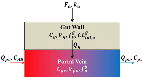
• Gut Compartment:

The gut compartment is composed of two sub-compartments [16]; the gut wall and the por-tal vein sub-compartments (Fig 4). The model to describe the gut wall sub-compartment is similar to the liver model with a few differences including a homogeneous compartment with a first order absorption, differences in enzyme levels and convection to the portal vein. Therefore the concentration of drugs and enzymes within the gut wall are described by:

dCg dt ¼

Xn_Dose

i¼1

FaDika Vg

expð k_aðt T_iÞÞHðt T_iÞ

½ðkg cat=K

g m;1þk

g inact=K

g IÞEgŠ f

g uCg

Vg max;2 Kg

m;2þf g uCh

fguCg Qg

Vg fguCg

dETot;g dt ¼k

g

deg 1þ

ðFIg max 1Þ ECg

50þ ðf g uCgÞ1

tr

nE

!tr

ðfg

uCgÞ ETot;g 1þ 1 kg_deg

kginact Kg

I

tr

ðfguCgÞ

1þ 1

Kg m;1

þ 1

Kgi

þ 1

Kg I

!tr

ðfguCgÞ

0 B B B B B @ 1 C C C C C A 2 6 6 6 6 6 4 3 7 7 7 7 7 5 Eg ¼

ETot;g

1þ 1

Kg m;1

þ 1 Kg i þ 1 Kg I !tr

ðfg uCgÞ

ð18Þ 8 > > > > > > > > > > > > > > > > > > > > > > > > > > > > > < > > > > > > > > > > > > > > > > > > > > > > > > > > > > > :

whereCgis the concentration of drugs in the gut wall,Fathe fraction absorbed of the drugs, Dithe dose at timeTi,kathe absorption rate constant of the drugs,nDosethe total number of doses given,fguthe fraction of unbound drugs in the gut wall,Vgthe volume of the gut wall,

Hthe Heaviside function andE_gandE_Tot;gare the free and total normalized enzyme levels to the initial and basal enzyme level in the gut wall;E0,g.Qgis a hybrid parameter introduced by Yang [17], which takes into account the membrane permeability of the drugs and blood flow from the enterocytes to the portal vein (seeS3 Appendixfor more details). All other parame-ters, exceptVg

max;2andE0,g, are taken equal to the corresponding liver values. The concentration within the portal vein sub-compartment is given by:

dC_pv dt ¼

Qpv

Vpv

CAB Cpv

þQg Vpv

fguCg ð19Þ

whereCpvis the concentration in the portal vein,Qpvthe blood flow of the portal vein and

Vpvthe volume of the portal vein.

• Liver Compartment:

Finally the liver compartment is described by the liver model previously described with the

boundary conditionC0ðtÞ ¼

QhaCABðtÞ þQpvCpvðtÞ

QhaþQpv

blood flows used for the simulation are taken as the average value of a 70 kg man and are summarized inS1 Table

Numerical resolution

To resolve the herein PBPK, a program was written in MATLAB1R2015b [18], using an object-oriented programming (OOP) approach. First, each compartment was identified as a generic

object which generates a functionfisuch as

dY_i

dt ¼fðt;YiÞwherefiandYiare both column vectors and represent the dynamics of the system and variables of interest (e.g. blood concen-tration and enzyme level) of the compartmenti, respectively. Then, the compartments are combined in a larger object that connects them with their respective blood flows; used to iden-tify the source term for each compartment, and generate a generic functionf(t,Y) such as dY

dt ¼fðt;YÞwheref

tr

¼ ðftr

1;f

tr

2;. . .;f

tr

nÞandY

tr_{¼ ðY}tr

1;Y

tr

2;. . .;Y

tr

nÞ. Finally,Y is resolved

by using the solverode15s, which was the preferred solver as it can solve stiff problems and adapt the time step for optimum resolution. A more detailed description of the main architec-ture of the program can be found in the appendixS6 Appendixand the code with an example in appendixS1 Code.

Parameters

Clinical studies. Ten clinical studies, summarized inTable 2, were selected to assess the predictions from the PBPK model with the observations. For each clinical study, midazolam was used to probe the impact of the perpetrator drug on the CYP3A4 enzyme.

Fig 4. The gut-compartmental model. The gut compartment is composed of two compartments; the gut wall and the portal vein sub-compartments. After an oral administration of a given drug, a fraction Fais absorbed from the intestine to the gut wall with an absorption rate

constant ka. Once the drug is in the gut wall, it may be metabolized and will cross the cell membrane (passively or actively) at a flow Qg,

depending on drug permeability and villous blood flow (seeS3 Appendix), to join the blood circulatory system. Once the drug is in the blood, it goes to the liver through the portal vein.

CYP3A4 enzyme. The CYP3A4 enzyme was the enzyme of interest, as it is the main

enzyme to metabolize midazolam. The amount of the CYP3A4 enzyme in the liver and intes-tine was taken as equal to 9.228μmol [8] and 0.070μmol [8], respectively. To estimate the con-centrationsE0andEg0for CYP3A4, the respective amounts were divided by the total volume of hepatocytesVh, estimated from the liver model, and the gut wall volume given inS1 Table. The degradation rate constantskdegandkgdegfor CYP3A4 were taken equal to 0.0192 h

−1_[29]

and 0.0288 h−1[29] for the liver and intestine, respectively.

Hepatic clearance. In the PBPK model, three parameters,kcat,Vmax,2andVmaxg ;2, were introduced. The hepatic blood clearanceCLHcan easily be obtained from clinical studies, which represents the clearance due to drug metabolism in the liver with respect to the blood compartment. Therefore,CLHwas corrected to estimate the three parameters. This is done first by estimating the apparent intrinsic clearanceCLintassuming a parallel tube model [9], due to the similarity with the herein liver model. Then to correct the impact due to exchange mechanisms between blood and hepatocytes, the metabolic intrinsic clearanceCL

int[30] was calculated. The equations forCLintandCLintare:

CLint ¼

QLiver

fb u

ln 1 CLH

QLiver

CL int ¼

SexðPþroutÞCLint

SexðPþrinÞ CLint

8 > > > <

> > > :

ð20Þ

wherefb

u andSexare the blood fraction unbound and the total exchange surface between blood and hepatocytes given by the liver model, respectively. Finally,kcat,Vmax,2andVmaxg ;2can be

Table 2. Summary of 10 in vivo clinical studies used in comparison to the simulations.

Perpetrator Dosage Regimen (p.o) Victim Dosage Regimen (p.o) Observation Ref.

Dose Numbers Interval Dose Intake Time Ratio

(mg) (mg) (h) AUCa _C

maxb

Azithromycin 500 3 doses q.d.c Midazolam 15 49.5 1.27 1.29 [19]

Cimetidine 400 3 doses Irregulard Midazolam 15 25 1.35 1.26 [20]

Clarithromycin 500 13 doses b.i.d.e _{Midazolam 8 144 8.39 3.80 [21]}

Diltiazem 60 5 doses t.i.d.f _{Midazolam 15 25 3.75 2.05 [22]}

Ethinyl Estradiol 0.03 10 doses q.d. Midazolam 7.5 217 1.20 1.16 [23]

Fluconazole 400 1 doses q.d. Midazolam 7.5 2 3.50 2.50 [24]

Fluoxetine 60 & 20 5 & 7 doses q.d. Midazolam 10 265 0.84 1.11 [25]

Ketoconazole 400 4 doses q.d. Midazolam 7.5 73 15.90 4.09 [26]

Pleconaril 400 15 doses t.i.d. Midazolam 5 112 0.65 0.76 [27]

Rifampin 600 10 doses q.d. Midazolam 5.5 Multipleg 0.12 0.17 [28]

a_{AUC: Area Under the CurveAUC¼}þ1R 0

CðtÞdt

b_{Maximum Concentration:C}

max¼max t0

CðtÞ

c

q.d.: quaque die (once a day) d

Intakes at 0, 12 and 24.5 h.

e

b.i.d.: bis in die (twice a day) f

t.i.d.: ter in die (three times a day) g

Intakes at 118 and 190 h.

calculated by:

kcat ¼fm;3A4

CL intKm;1

E0Vh

V_max;2 ¼ ð1 fm:3A4Þ

CL intKm;2

Vh

Vmaxg ;2 ¼

ð1 f3A4g ÞA g CYPVGW

ð1 f_3A4ÞA_CYPV_h Vmax;2

8 > > > > > > > > <

> > > > > > > > :

ð21Þ

wherefm, 3A4is the fraction metabolized by the CYP3A4 enzyme,ACYPandA g

CYPare the total amount of CYP in the liver and intestine, respectively, andf3A4andf

g

3A4are the fraction amount of CYP3A4 in the liver and intestine, respectively. Hepatic and intrinsic clearances CLH/CLint/CLintand fraction metabolizedfm, 3A4are reported inTable 3, blood fraction unboundfb

u inTable 4, and fraction amountsf3A4/f3A4g and CYP amountsACYP/AgCYPin TableS2 Table.

Renal clearance. The renal clearance valuesCLRwere obtained from the literature (Table 3). As the renal clearance is expressed with respect to the blood compartment, as it is the case for hepatic clearance, an intrinsic renal clearanceCLint,Rwas calculated by assuming a well-stirred model [9]. The intrinsic renal clearanceCLint,Rcan be expressed as:

CLint;R¼

RBP

Kp;K

QKCLR

QK CLR

ð22Þ

whereQK,RBPandKp,Kare the kidney blood flow (S1 Table), the blood-to-plasma ratio (Table 4) and the kidney partition coefficient (Table 5), respectively.

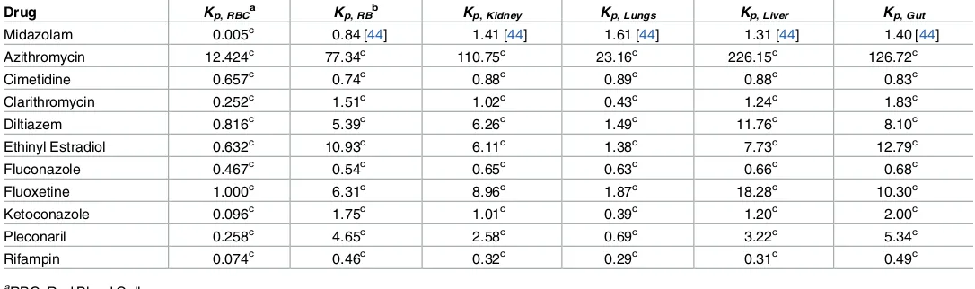
Remaining parameters. The partition coefficients for each compartment and drug are

found inTable 5. Parameters related to reversible inhibition, MBI and induction are reported

Table 3. Metabolism parameters of the drugs.

Drug CLH CLm, int CLm;int Km fm, 3A4 CLR

L/h L/h L/h μM L/h

Midazolam 34.42 [31] 1095.19 1991.20 2.30 [32] 0.96 [33] 0.09 [5]

Azithromycin 33.60a 353.81 392.18 150.00 [29] 1.00b 9.29a

Cimetidine 13.44 [34] 16.22 16.83 10.00c 0.00 17.22a

Clarithromycin 26.52 [31] 112.47 131.30 50.00d _{0.80 6.00 [31]}

Diltiazem 50.20a,e _{340.21 375.54 30.00}d _{1.00 [35] 2.88}a

Ethinyl Estradiol 42.52a 1643.00 5334.34 18.00d 0.60 [36] 0.00

Fluconazole 0.71 [37],e 0.80 0.80 10.00c 0.00 1.03a

Fluoxetine 40.32 [38] 1083.31 1546.61 10.00c _{0.00 0.00}

Ketoconazole 0.69 50.74 [4] 51.46 1.52 [4] 0.00 0.00

Pleconaril 24.29 [39] 1953.50 4248.41 10.00c 0.00 0.00

Rifampin 8.66a 50.45 51.17 10.00c 0.00 1.68a

a

Average value from PharmapPendium®database:www.pharmapendium.com

b

DrugBank.

c

Assumed.

d

Assumed to be Equal to Kiwhen fm, 3A4is not equal to 0. e

inTable 6for each drug, whereas fraction absorbedFa, absorption constant rateka, the hybrid gut wall flowQg, and the permeabilityPfor each drug are shown inTable 7. Finally, it is assumed that there is no active hepatocyte uptake or efflux for all drugs considered in this pres-ent work (i.e.ρin= 0 andρout= 0).

Table 5. Tissue-to-plasma partition coefficients of the drugs.

Drug Kp, RBC

a

Kp, RB b

Kp, Kidney Kp, Lungs Kp, Liver Kp, Gut

Midazolam 0.005c 0.84 [44] 1.41 [44] 1.61 [44] 1.31 [44] 1.40 [44]

Azithromycin 12.424c _77.34c _110.75c _23.16c _226.15c _126.72c

Cimetidine 0.657c _0.74c _0.88c _0.89c _0.88c _0.83c

Clarithromycin 0.252c 1.51c 1.02c 0.43c 1.24c 1.83c

Diltiazem 0.816c 5.39c 6.26c 1.49c 11.76c 8.10c

Ethinyl Estradiol 0.632c _10.93c _6.11c _1.38c _7.73c _12.79c

Fluconazole 0.467c _0.54c _0.65c _0.63c _0.66c _0.68c

Fluoxetine 1.000c 6.31c 8.96c 1.87c 18.28c 10.30c

Ketoconazole 0.096c 1.75c 1.01c 0.39c 1.20c 2.00c

Pleconaril 0.258c _4.65c _2.58c _0.69c _3.22c _5.34c

Rifampin 0.074c _0.46c _0.32c _0.29c _0.31c _0.49c

a_{RBC: Red Blood Cells.} b

Estimated by averaging the partition coefficients of the remaining tissues:Kp;RB¼

Xn

i¼1 ViKp;i=

Xn

i¼1

Vi(seeS5 Appendixfor equation development). c

Theoretical values estimated using the equations by Rodgers and Rowland. Two formula were used; one for the moderate to strong bases (pKa>7) and

the group 1 zwitterions (pKa,1>7) (Rodgers et al. 2005) and the second for acids, neutrals, weak bases (pKa<7) and group 2 zwitterions (pKa,1<7)

(Rodgers et al. 2006). The parameters used in these equations are given inS3andS4Tables.

https://doi.org/10.1371/journal.pone.0183794.t005

Table 4. Fraction unbound and blood-to-plasma ratio of the drugs.

Drug fp

u f

b

u RBP f

h u

a _fgw

u

a

Midazolam 0.0264 0.0400 [34] 0.66 [31] 0.0202 0.0189

Azithromycin 0.7000 [40] 0.1200 [41] 5.83b 0.0031 0.0055

Cimetidine 0.8730 0.9000 [34] 0.97 [42] 0.9880 1.0000

Clarithromycin 0.1800 [31] 0.2813 0.64 [42] 0.0122 0.0984

Diltiazem 0.2028 0.2200 [34] 0.92 [43] 0.0173 0.0251

Ethinyl Estradiol 0.0300c 0.0355 0.84b 0.0039 0.0023

Fluconazole 0.6893 0.8900 [41] 0.77b 0.1051 1.0000

Fluoxetine 0.0500 0.0500 [41] 1.00d _{0.0057 0.0049}

Ketoconazole 0.0095 [43] 0.0136 0.70 [43] 0.0075 0.0048

Pleconaril 0.0100c 0.0146 0.69b 0.0041 0.0019

Rifampin 0.1100c 0.1809 0.61b 0.3513 0.2234

a fh

u ¼ fp

u Kp;Liver

andfgw u ¼

fp u Kp;Kidney b_R

BP= h×Kp, RBC+ 1−h where h = VRBC/VBloodis the hematocrit coefficient.

c_{DrugBank database:www.drugbank.ca} d_Assumed.

Table 6. Interaction parameters of the drugs.

Drug Inhibition MBI Induction

Ki kinact KI FImax EC50 EC50

a

μM h−1 μM μM μM

Azithromycin 150.00 [29] 0.30 [7] 19.00 [7] 1b ₊₁b ₊₁

Cimetidine 115.00 [29] 0b ₊₁b ₁b ₊₁b ₊₁

Clarithromycin 50.00 [29] 3.18 [29] 18.90 [29] 1b +1b +1

Diltiazem 30.00 [29] 1.68 [29] 1.15 [29] 1b +1b +1

Ethinyl Estradiol 18.00 [7] 2.40 [7] 18.00 [7] 70.00 [7] 20.00 [7] 3.33

Fluconazole 3.40 [29] 0b ₊₁b ₁b ₊₁b ₊₁

Fluoxetine 8.00 [29] [29] 0.61 [29] 3.10 [29] 0.54 [29] 0.18

Ketoconazole 0.006 [29] 0b +1b 1b +1b +1

Pleconaril +1 0b ₊₁b _{34.00 [45] 16.40 [45] 3.83}

Rifampin 100.00 [29] 0b ₊₁b _{34.00 [29] 0.57 [29] 0.54}

a_EC

50was corrected to take into account fraction unbound in incubation, permeability and active transport where:EC50¼fu;inc

S_exðPþr_inÞ

SexðPþroutÞ þCL

int

EC50, Sex= 10046 dm2is given by the liver model and fu, incis calculated theoretically by using the formula by Kilford et al. 2008.

b

Not known as being a reversible inhibitor, MBI inhibitor or inducer. If not a reversible inhibitor Ki= +1, if not a MBI inhibitor kinact= 0 and KI= +1and if not

an inducer FImax= 1 and EC50= +1.

https://doi.org/10.1371/journal.pone.0183794.t006

Table 7. Fraction absorbed, absorption constant rate, Qgand permeability of drug chemicals.

Drug Fa ka Qga P

h−1 _{L/h μm/h}

Midazolam 1.00b _{1.16 [31] 15.44 24228.0 [15]}

Azithromycin 0.86 [31] 0.11 [31] 20.51 36000.0b

Cimetidine 1.00b 1.00b 2.57 4468.6 [46]

Clarithromycin 0.55 [47] 1.08 [31] 4.77 7807.8 [48]

Diltiazem 1.00 [8] 1.60 [8] 18.41 36000.0b

Ethinyl Estradiol 1.00b 1.00b 15.13 23635.9 [36]

Fluconazole 0.86 [37] 0.88 [37] 6.23 13646.5 [46]

Fluoxetine 1.00b _1.00b _{22.29 36000.0}b

Ketoconazole 1.00b _1.00b _{23.34 36000.0}b

Pleconaril 0.70c 1.00b 23.31 36000.0b

Rifampin 1.00b 1.00b 19.18 36000.0b

a_Q g¼

CLpermQv fb_u

CLpermþQv

fb_u

: seeS3andS4Appendices for more details.

b_Assumed.

c_{DrugBank database:www.drugbank.ca} https://doi.org/10.1371/journal.pone.0183794.t007

Table 8. Sinusoids length for each level.

Level Length

μm

1 344.8

2 185.3

3 92.5

4 46.0

5 22.5

Total 691.1

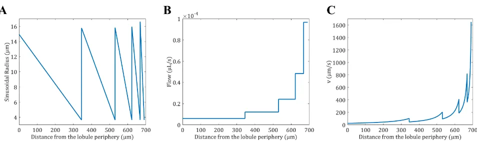
Fig 5. Properties of 5 sinusoid levels from the lobule model. (A) The radius of the sinusoids is expressed as a function of the distance to the periphery of the lobule. For a given level, the radius is decreasing as the sinusoids are converging toward the center of the lobule. Once the sinusoids reach their minimum size they merge together which increases the radius size in a stepwise manner. (B) The flow of the sinusoids is expressed as a function of the distance to the periphery of the lobule. For a given level, the flow is constant, but double when two sinusoids merge. (C) The velocity of the sinusoids is expressed as a function of the distance to the periphery of the lobule. For a given level, the velocity is increasing as the sinusoid radius is decreasing. Once the sinusoids reach their minimum size they merge which decreases the blood velocity suddenly.

https://doi.org/10.1371/journal.pone.0183794.g005

Fig 6. Simulated PK of the perpetrator (blue) and victim (orange) drugs. The simulation were run using the clinical dose regimens from

Table 2: (A) Azithromycin (B) Cimetidine (C) Ethinyl Estradiol (D) Rifampin.

Results

Algorithm construction of liver

The algorithm to construct the lobule geometry generated 5 sinusoidal levels, where the length of each level is represented inTable 8. The volume of one lobule and the number of lobules, estimated from the parameters inTable 1, are respectively 4.06× 107_μm3

and 4.16× 107

. Given the average liver volume of 1.69 L for a man of 70 kg (S1 Table), the construction of the lobules respecting the algorithm presented inFig 1Cgave a total hepatocytes volume Vh= 1392 mL and blood volumeVb= 283 mL. Therefore the liver volume given by the model is 1.67 L, which is slightly less than the input volume. Similarly the blood content can be com-pared to the literature which varies between 250 mL and 312 mL [49]. Furthermore, the sur-face exchange between blood and hepatocytesSexgiven by the model was estimated to be

Fig 7. Simulated enzyme levels as a function of time. The total enzyne level (free enzyne + enzyme-substrate complex) is represented as a fold change compared to the initial level. The color gradient indicates the positions within the lobule from blue (Entrance of the lobule) to red (Exit of the lobule): (A) Azithromycin (MBI inducer) (B) Cimetidine (Reversible inhibitor: No effect on enzyme level) (C) Ethinyl Estradiol (MBI inhibitor and inducer: It seems that in this case the effect cancels each other out) (D) Rifampin (Inducer).

10046 dm2, which is expected to influence the calculation ofCL

intfromin vivodata. Finally, assuming a cell volume ofVcell= 4μL/106cells [50], the number of hepatocytes per liver is 348× 109cells which is equivalent to 193× 106cells/g of liver. This compares well to the litera-ture values which range from 65 to 185× 106cells/g of liver [51].

The mathematical construction of the lobule gives the radius of the sinusoids for each level as represented inFig 5A. Given the number of lobules and the blood flow in the liver, the blood flow for each sinusoid level can be estimated by dividing the total blood flow by the total number of sinusoids at a given level as represented inFig 5B. From the liver blood flow and the radius of the sinusoids, the velocity in the sinusoids (Fig 5C) was calculated as the ratio of the sinusoids flow to the cross section area as follows:v(x) =Q(x)/S(s), where the cross section area of the sinusoids is expressed asS(x) =R(x) (eL− 2RH) (seeS1 Appendix).

Simulations and comparisons

The clinical data presented inTable 2were simulated and the PK profiles of the victim and perpetrator drugs are represented inFig 6. In addition to the PK profiles, the model simulates

Fig 8. Simulated PK profile for midazolam after an oral dose of 15 mg and comparison to clinical data. (?) Fee et al. 1987 [20] (•) Zimmermann et al. 1996 [19].

the enzyme level in the liver and gut wall as a result of the different mechanisms involved in drug metabolism. The enzyme levels as a function of time in the liver are given inFig 7, where the spatial effect is also represented with a color gradient. Furthermore, the PK profile of mida-zolam alone was simulated and compared to clinical data inFig 8. The model seems to ade-quately predict midazolam PK. Finally, the PK profiles of midazolam with a placebo and the perpetrator for each of the clinical studies inTable 2are represented inFig 9and a comparison of the prediction and clinical observation of theAUCratioandCmax,ratioare summarized in Table 9. Fold error in eight out of ten predictions are within 2-fold which is a common criteria for good prediction [29,52]. InFig 10the observedAUCratioare plotted against the predicted

AUCratio. Most of the predictions are relatively well aligned with the line of unity except for the pleconaril scenario where the induction was overpredicted, thereforeAUCratiounderpredicted. AnR2of 0.85 was calculated which indicates a good correlation between the observations and the model predictions.

Fig 9. Simulated PK profiles for midazolam with a placebo (blue) or a perpetrator (orange) and comparison to clinical data. The dots represent the clinical observations: (A) Azithromycin [19] (B) Cimetidine [20] (C) Ethinyl Estradiol [23] (D) Rifampin [28].

Discussion

The objective of this work was to develop a mathematical model to predict PK drug-drug interactions in a dynamic manner which may occur in the liver and the intestine. The main focus was on the liver, as the majority of drug metabolism and therefore DDIs occur in this organ. However, to incorporate first pass metabolism the intestine was also included. The main results from this work are; (i) the liver model is capable of describing the geometry of a lobule in a simple manner; (ii) the liver model can be incorporated into a PBPK model to pre-dict the PK profile of a drug; (iii) the PBPK model is, so far, capable of prepre-dicting the DDIs when one enzyme is mainly involved in DDIs. The novelty of the model presented in this work is the description of the lobule/liver geometry in the simplest manner possible to account for spatial variation in blood flow, concentrations and enzyme level. Furthermore, a cellular model was included to model drug transport,i.e. permeability, uptake and efflux, between blood and hepatocytes and drug metabolism within the hepatocytes, without creating a discon-tinuity with the historical models (e.g. the well stirred model [9] or parallel tube model [9]). It has the advantage of comparing the geometrical properties of the lobule generated by the model to physiological data such as the liver blood content, number of lobules, surface exchange, sinusoidal radius, velocity, blood flow profile and, the hydrodynamic pressure load. More detailed geometries have been proposed [14,53,54], but their implementation into a pharmaceutical context is not optimal as it is demanding in computational resources (comput-ing power and scientific IT support). Therefore it seems that the liver model herein is an appropriate compromise between the complexity of the model and its implementation. The calculated blood content in the liver (excluding arteries and veins) is in the range of literature values which varies between 250 mL and 312 mL [49]. However, the number of cells per gram of liver is relatively higher than the literature values which range from 65 to 185× 106cells/g of liver [51]. As it was assumed that the hepatocyte plates are homogeneous, the space of Disse and other cell types (e.g. Kupffer cells) were neglected which could have lead to an overestima-tion of the number of hepatocytes. Based on the lobule geometry, the surface estimated for

Table 9. DDI prediction for the 10 clinical studies.

Drug AUCratio Cmax, ratio

Perpetrator Victim Observation Prediction F.E.a _{Observation Prediction F.E.}a

Azithromycin Midazolam 1.27 1.16 1.10 1.29 1.08 1.20

Cimetidine Midazolam 1.35 1.32 1.02 1.26 1.20 1.04

Clarithromycin Midazolam 8.39 5.36 1.57 3.80 2.24 1.69

Diltiazem Midazolam 3.75 7.52 2.01 2.05 2.37 1.16

Ethinyl Estradiol Midazolam 1.20 1.00 1.20 1.16 1.00 1.16

Fluconazole Midazolam 3.50 4.85 1.38 2.50 2.15 1.16

Fluoxetine Midazolam 0.84 1.56 1.85 1.11 1.27 1.14

Ketoconazole Midazolam 15.90 18.17 1.14 4.09 3.09 1.33

Pleconaril Midazolam 0.65 0.12 5.30 0.76 0.24 3.17

Rifampin Midazolam 0.12 0.12 1.02 0.17 0.26 1.56

GMFEb _{1.52 GMFE}b _1.38

a

Fold Error¼10 log Ob

Pred

b

GMFE: Geomtric Mean Fold ErrorGMFE¼10

PN

i¼1log

Obi Pred_i

exchangesSexmight have been underestimated as it is half of the maximum surface of exchange; assuming that the surface of all the cells is in contact with blood, which in turn is expected to influence the calculation of the metabolic intrinsicCL

intobtained fromin vivodata for low permeable drugs. A comparison ofin vivoandin vitrodata across a range of drugs may allow to estimate a more realistic value ofSex. Finally, the pharmacokinetic profile of midazo-lam was relatively well predicted as well as the impact of the perpetrator drug on itsAUCand Cmax. Indeed theGMFEAUCwas estimated to 1.52 which is in the lower range of literature val-ues (1.47–2.5 [7,29]). A comparison to the static combined model by Fahmiet al. [7] and to a well-stirred model similar to the DDI model by Rowland-Yeoet al. [8] was also made (results not shown) where theGMFEAUCwere estimated at 2.55 and 1.71, respectively, which suggests that dynamic models are far superior to static models and that geometry might help to improve predictions. However, it is worth noting that the herein results were estimated with-out taking into account hepatic uptake, which generally improves predictions [55], and with-out fitting any parameters. All parameters were taken from the literature or calculated using published algorithms. Ideally, each parameter should be estimated experimentally in a specific in vitroassays, where it is assumed that they are representative of what is happeningin vivo.

Fig 10. Observed AUCratioversus predicted AUCratio. The solid line represents the line of unity, the dashed lines are the 2-fold errors and

the dotted lines the 5-fold errors.

This point needs careful consideration as measuring the drug-metabolizing ability of isolated hepatocytes leads very often to under-predictions of drug clearance. Moreover, studies have shown that an oxygen gradient [56,57] and blood flow [58] (i.e. shear stress) affect the expres-sion levels of CYPs. The liver model shows that the blood flow inside the liver is non-linear due to its hierarchical anatomical structure and may explain the notion of zonation,i.e. CYPs are more highly expressed in certain zones of lobules compared to others. Both effects could be incorporated into the model, where the oxygen concentration and the variation in shear stress, related to changes in velocity in a lobule, can be modeled.

Conclusion

A liver model including a simple description of the lobule geometry and the uptake/efflux transport between the blood and hepatocytes was presented. The model predicts the pharma-cokinetic profiles, enzyme activity and drug-drug interaction for different type of DDIs. Future research will test the model with two or more enzymes involved in metabolism to validate the model further, take into consideration uncompetitive, non-competitive or mixed inhibition and potentially add a component for the biliary excretion which is not negligible for some drugs. Furthermore, the model needs to be compared to models with increasing complexity, i.e. from static models to dynamic model, to assess how the new features of the herein model improves DDI predictions. Finally, this research focused on the liver as it is the main organ involved in drug metabolism, but the intestine and kidneys may play a significant role in DDIs. Therefore combining the herein liver model to a more sophisticated gut model (e.g. the advanced compartmental absorption and transit (ACAT) model) and/or a kidney model, where transporters are taking into account, could potentially improve the prediction of DDIs in the future.

Supporting information

S1 Appendix. The geometry of sinusoids. Description of how the the parametersαB!H(x) andαH!B(x) were obtained.

(PDF)

S2 Appendix. Model simplification. Detailed descriptions on how Eqs (10) and (12) were obtain from Eqs (7) and (11).

(PDF)

S3 Appendix. The hybride parameterQg. The two definitions of the parameterQgby Yang

et al. [17] and Hisakaet al. [16] are presented. (PDF)

S4 Appendix. Hisaka equation forQg. Description of howQgis deduced by Hisakaet al. [16]. (PDF)

S5 Appendix. Average partition coefficient. Description of how the partition coefficient of a

PK compartment composed of different tissues is calculated. (PDF)

S6 Appendix. Numerical resolution and OOP. A brief description of Object-Oriented

Pro-gramming (OOP) and a detail description on the program to solve the PBPK model. (PDF)

S1 Table. Average volume and blood flow for a 70 kg man for different tissues.

S2 Table. Amounts and degradation rate constants for different CYP enzymes in the liver and the intestine.

(PDF)

S3 Table. Physico-chemical properties of the drugs. Physico-chemical parameters used to

calculate the partition coefficients. (PDF)

S4 Table. Composition of human tissue for different organs. Tissue composition used to

calculate the partitions coefficient. (PDF)

S1 Code. Matlab code. The code of all the objects used for the simulations and an example on

how to use them to solve a PBPK model. (RAR)

Author Contributions

Conceptualization: Mohammed H. Cherkaoui-Rbati, Stuart W. Paine.

Data curation: Mohammed H. Cherkaoui-Rbati.

Formal analysis: Mohammed H. Cherkaoui-Rbati.

Funding acquisition: Stuart W. Paine, Cyril Rauch.

Investigation: Mohammed H. Cherkaoui-Rbati.

Methodology: Mohammed H. Cherkaoui-Rbati, Stuart W. Paine, Peter Littlewood, Cyril

Rauch.

Project administration: Stuart W. Paine.

Resources: Peter Littlewood.

Software: Mohammed H. Cherkaoui-Rbati.

Supervision: Stuart W. Paine, Peter Littlewood, Cyril Rauch.

Validation: Mohammed H. Cherkaoui-Rbati, Stuart W. Paine, Peter Littlewood, Cyril Rauch.

Visualization: Mohammed H. Cherkaoui-Rbati.

Writing – original draft: Mohammed H. Cherkaoui-Rbati.

Writing – review & editing: Stuart W. Paine, Peter Littlewood, Cyril Rauch.

References

1. Huang SM, Strong JM, Zhang L, Reynolds KS, Nallani S, Temple R, et al. New era in drug interaction evaluation: US Food and Drug Administration update on CYP enzymes, transporters, and the guidance process. J Clin Pharmacol. 2008; 48(6):662–670.https://doi.org/10.1177/0091270007312153PMID:

18378963

2. Routledge PA, O’Mahony MS, Woodhouse KW. Adverse drug reactions in elderly patients. British Jour-nal of Clinical Pharmacology. 2004; 57(2):121–126.https://doi.org/10.1046/j.1365-2125.2003.01875.x

PMID:14748810