Design framework for multifunctional additive manufacturing: placement and routing of three dimensional printed circuit volumes

A. Panesar

Faculty of Engineering, University of Nottingham, University Park, Nottingham NG7 2RD, UK e-mail: [email protected]

D. Brackett

Faculty of Engineering, University of Nottingham, University Park, Nottingham NG7 2RD, UK

I. Ashcroft

Faculty of Engineering, University of Nottingham, University Park, Nottingham NG7 2RD, UK

R. Wildman

Faculty of Engineering, University of Nottingham, University Park, Nottingham NG7 2RD, UK

R. Hague

Faculty of Engineering, University of Nottingham, University Park, Nottingham NG7 2RD, UK

Design Framework for

Multifunctional Additive

Manufacturing: Placement and

Routing of Three-Dimensional

Printed Circuit Volumes

A framework for the design of additively manufactured (AM) multimaterial parts with em-bedded functional systems is presented (e.g., structure with electronic/electrical compo-nents and associated conductive paths). Two of the key strands of this proposed framework are placement and routing strategies, which consist of techniques to exploit the true-3D design freedoms of multifunctional AM (MFAM) to create 3D printed circuit volumes (PCVs). Example test cases are presented, which demonstrate the appropriate-ness and effectiveappropriate-ness of the proposed techniques. The aim of the proposed design frame-work is to enable exploitation of the rapidly developing capabilities of multimaterial AM. [DOI: 10.1115/1.4030996]

1

Introduction

A multifunctional part has multiple uses, such as structural and electrical functions, for example, a structural health monitoring part. Multifunctional designs could be realized using AM multi-material processes, and allow for a new AM design paradigm. The manufacturing processes, such as multihead ink jet printing, capable of producing these parts are still under development, with considerable ongoing research into materials and process configu-ration. A variety of techniques have been proposed, primarily using stereolithography and direct write/print technologies, and the reader is directed to Lopes et al. [1] for a history of work car-ried out in this area. As this area of manufacturing is nascent, there has been little work carried out on developing the design philosophies tailored for MFAM, particularly within the scope of optimal placement and routing. Some related works to define design for AM (DfAM) frameworks are the multimaterial design framework: OpenFab [2] that defines a procedure to efficiently grade mechanical properties through the volume of a part; and a three step global approach to DfAM [3], which is more general.

The aim of this work is to define the underlying design frame-work for MFAM, outline and formalize a set of techniques/ methods that aid the design of a multifunctional part. The multi-material manufacturing capability expands the possible design freedom from purely design of single material boundary geometry to also include material composition and functionality through the volume of the part. Two conceptual examples of multifunctional components are shown in Fig.1, consisting of placed components and the associated connections routed between them within a

structural part, two of the key strands of the overall design for MFAM framework.

Automated placement and/or routing techniques have been employed in numerous fields, including electronics, civil (build-ings), aerospace, navigation systems, and artificial intelligence (robotics). The electronics community has benefited significantly from advancements in these techniques and this is evident from the highly miniaturized and optimized very large scale integration (VLSI) and printed circuit board (PCB) designs. The continual need to improve these designs has led to the maturation of the underlying multiphase process: partitioning (breaking the original problem into subproblems), placement, and routing. In general, the tasks for PCB design consist of: (1) logical design, (2) physi-cal layout, and (3) production, with stage two consisting of com-ponent placement and wire routing [5]. In principle, it would be

Fig. 1 Multimaterial jetted concept prototype: (a) an example of a topologically optimized structural part with integrated in-ternal system of placed components and the associated rout-ing, and (b) a prosthetic arm with embedded systems and the associated connections between components [4]

best to perform placement and routing in one coupled step as placement can have significant repercussions on the routing, but due to nested dependencies, these can be best tackled independ-ently (in terms of computational expense). To this end, several graph algorithms and mathematical methods, as reported in Refs. [5–7], have been developed and implemented. Many of these strategies have been adapted and coupled with global optimization algorithms, such as genetic algorithms and ant colony optimiza-tion (ACO), to solve optimizaoptimiza-tion problems in other fields. Exam-ples include pipe/cable routing problems [8–11] and optimum placement problems for structural health monitoring [12,13].

Currently, PCBs within electronic devices are limited to a stacked 2D (i.e., 2.5D) paradigm [14]; however, with the develop-ment of multimaterial AM, the design of functional devices in true 3D, termed PCVs, can be considered. The 3D placement of internal components and the associated routing of connecting tracks should enable more compact, better integrated, and capable MFAM systems.

The objectives of this work can be summarized as:

(1) to devise a suitable framework to enable the design of mul-tifunctional parts

(2) to devise a suitable strategy to determine suitable locations for the internal components

(3) to devise a suitable strategy to connect the internal compo-nents into a circuit

This paper takes the following structure: First, the overall framework is introduced. Second, the placement and routing

aspects of this framework are detailed. Third, the effectiveness and appropriateness of the proposed methods are demonstrated by evaluating and discussing the results for some example test cases.

2

Methodology

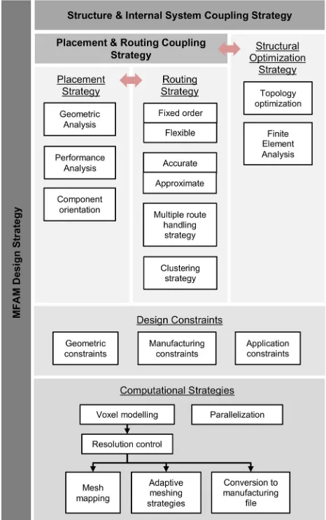
2.1 Overall Framework.The overall optimization-based design framework for MFAM is shown in Fig.2and has three pri-mary strands within the structure and internal system coupling strategy: First, the placement of components within the part, second, the routing between these components, and third, accom-modating the effect of integrating these components on the struc-tural response of the part by modification of the structure using an optimization strategy. It is worth realizing that the placement and routing within a PCV do not necessarily need to operate at the level of a traditional PCB design process, as for some applica-tions, the scale is such that consideration of the minutiae of PCB design is prohibitive and unnecessary. In these cases, the design of an existing circuit can be considered as a component in itself to be connected up with others within the parts’ volume. Overarch-ing these three strands are the couplOverarch-ing strategies to consider interactions between them. Completing the MFAM design strat-egy is the incorporation of design constraints and strategies employed for efficient and flexible computation of results. Sec-tions2.1.1–2.1.4will elaborate on the above outlined key aspects of the optimization-based design framework of Fig.2specifically: placement and routing strategies, coupling strategies, design con-straints, and computational strategies.

2.1.1 Placement and Routing Strategies.The aspects of this overall framework that are the focus of this paper are the place-ment and routing strategies. The key aspects of the placeplace-ment strategy are: identification of potential suitable locations through geometric and performance analysis; identification of a suitable orientation for the component under consideration; and finally, assessment of the location suitability for this component by check-ing whether it fits within the available space. The key aspects of the routing strategy are: separating the components by connection type; computing shortest paths for pairs of components; and finally, solving the combinatorial network problem (if one exists). These methods are detailed in Secs.2.2and2.3.

2.1.2 Coupling Strategies.The three primary strands of Fig.2 are used to formulate a coherent design procedure by devising suitable coupling strategies; specifically, the coupling between placement and routing, and the coupling between the structural optimization and the placement and routing. The first of these cou-plings could be achieved with a heuristic approach similar to those used for standard PCB or VLSI design [5], or a general purpose metaheuristic algorithm such as ACO. Addressing the second of these couplings, is an approach that incorporates the effects of placement and routing methods via the finite-element analysis (FEA) into a structural topology optimization (TO) algorithm, as detailed in the previous works [15,16]. TO is an optimization technique that iteratively improves the material layout within a given design space, for a given set of loads and boundary condi-tions [17–20]. In this approach, the effective material properties are used for the internal system, so as to reflect its part weakening or re-enforcing characteristics. These in turn can be determined by simulating a detailed material interface FEA.

multifunctional part being designed, there will also be specific manufacturing and application constraints that could be useful to include. For example, to minimize the support structure require-ments one may have to investigate the best build orientation while incorporating the repercussions, this may have on the relative ori-entation of components within the part. Generally speaking, this portion of the framework encompasses constraints applicable to any other portion of the framework. Specific constraints for place-ment and routing are discussed in more detail in Secs.2.2and2.3, where appropriate.

2.1.4 Computational Strategies.A voxel modeling environ-ment was used for this design framework, where a voxel repre-sents a point in space on a cuboidal grid. This was for three primary reasons:

First, the proposed placement and routing strategies require dis-cretization of the design volume to enable explicit identification and/or comparison of potential placement locations and routed paths.

Second, mesh mapping between different stages of the process is more straightforward, which provides for a high degree of con-trol of mesh resolution that can be used to optimize mesh resolu-tion for a particular process, or stage within a process. This multiresolution mesh mapping can be best achieved through the use of variable foreground meshes that are compatible with (i.e., an offspring of) a constant background mesh, and is termed multi-ple compatible mesh method (MCMM). To illustrate the useful-ness of the MCMM, consider an example where a fine resolution is used for structural optimization, a coarse resolution for place-ment and routing optimization, and a very fine resolution for

manufacturing. In doing so, the overarching design, optimization, and manufacturing process are made more efficient.

Third, the use of a voxel modeling environment allows the direct mapping of raster-based file formats used in AM, such as the bitmaps used in jetting. This eliminates the need for manual computer-aided-design (CAD) operations, including conversion to the common STereoLithography (STL) file format and associated slicing, which is well known to be cumbersome and error prone. Several stages of voxel manipulation including upsampling and smoothing are required to convert the output voxel model to a model manufacturable using a jetting process, but the model remains inherently sliced.

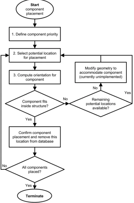
2.2 Placement Strategy.This section provides the detail on the placement strategy introduced in Sec.2.1.1. It consists of three key stages: determining component priority, identifying the com-ponent location, and identifying the comcom-ponent orientation. The overall placement strategy is summarized by the flow chart in Fig.3.

2.2.1 Stage 1: Component Priority.The first step in this pro-cedure is to define the priority of each component to determine the order in which they will be placed. This is achieved using the weighted mean of two measures: component size and component importance (dependent on its connectivity). Components are placed in descending order of this value.

2.2.2 Stage 2: Component Location.The identification of locations for evaluation of suitability for a component is deter-mined using two substages. The first substage identifies a choice of locations based on both geometric and performance characteris-tic analyses. The second substage assesses these locations for each component based on whether the component can fit at that location.

Stage 2a: identification of potential locations.A hierarchical approach to component placement location was defined as shown in Fig.4, which presents different point sets within the part’s vol-ume based on geometric analysis. Points are eliminated from these sets based on constraints of whether the dimensions of the compo-nent allow it to fit at that location, and a minimum spacing constraint to avoid components touching each other.

For some internal components, it is known in advance exactly where it should be placed (specific points). For other components, there may be some that need to be constrained to certain regions of the part (rather than the precise location predetermined), such as components that require access to the outside surface of the part for connectivity or heat dissipation requirements, and so should be constrained to surface locations only.

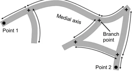
Another example is where the components might be required to be placed such that they are well encapsulated within the structure or to monitor the performance of geometric members, for exam-ple, for a structural health monitoring application. The compo-nents could then be placed on the medial axis, generated using skeletonization, which is the general name given to the process that reduces the quantity of geometric information (i.e., dimen-sionality) required to represent a structure while preserving the essence of its topology. In 3D, this involves simplification to a 2D medial surface and 1D medial axis. The medial surface and axis for the 3D geometry of Fig.5(a)are shown in Figs.5(b)and5(c),

Fig. 3 The placement strategy for MFAM design

respectively. A thinning algorithm, as detailed in Refs. [21,22], was used to obtain the skeletal information of the part’s topology, providing the characteristic geometric information. Using the medial axis information reduces the domain of component place-ment from a 3D volume to a network of 3D lines, thereby signifi-cantly reducing computational expense. For instance, to realize this dimensionality approximation, individual segments (approxi-mating each geometric member) can be extracted from the medial axis by dividing it at the joints of the skeleton. Once the member centerlines have been isolated, the points on these members can be used to form the potential locations for the placement of the in-ternal components. It is noteworthy that for bulky parts, the reduced geometric information obtained using skeletonization, although topologically intact, is only at the very best a rough approximation to the part’s local geometry as local member thick-ness is not included in this representation.

Another way of reducing the whole volume of points, for instances where there is no restriction to surface points, the medial axis or a specific point, is to use a domain decomposition tech-nique such as a Voronoi diagram. Voronoi-based domain decom-position can enable the identification of a set of approximately uniformly distributed points in 3D. The procedure for doing this involves: initially selecting a set of random points within the parts’ volume; constructing a Voronoi diagram from them; and then identifying the centroids of these regions which define the new point set (Fig.6).

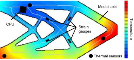
For many structures, the geometry plays less of a role in deter-mining the component location than the performance of the struc-ture either in response to some loading on the part or as a response to an external influence. For example, an internal system of components and sensors can be used to provide an assessment of the part’s performance in-service, enabling a more tailored maintenance schedule and thus reducing costs, or to enable some response to be carried out during use (“intelligent parts”). Analy-sis of the part’s performance can be utilized to identify appropri-ate component placement, for example, consider Fig. 7, which shows a structure subjected to an external heat source. In order to effectively monitor the thermostructural response of this structure, two thermal sensors are placed at the hot spots, a central process-ing unit (CPU) in the cold spot to process data from the sensors (accompanied by a thermal sensor to monitor the temperature of the CPU), and strain gauges in key structural members. This analysis is carried out using FEA.

The list of potential points is filtered based on a minimum spac-ing constraint, which ensures components do not overlap. This constraint is based on the maximum component dimension. Once

the potential points have been filtered based on spacing, for each component, the list is explored based on whether the component can fit at that location, based on the components’ smallest dimen-sion. The amount of space available at each location is determined by the radius of the maximal sphere (touching the part boundary). This is a prechecking procedure to provide an initial elimination of completely unsuitable points, prior to complete checking of dimensions taking orientation into account during stage 3.

2.2.3 Stage 3: Component Orientation.In Fig. 7, it can be observed that the components are oriented in directions that are influenced by the medial axis of the structure (geometric influ-ence). This is especially appropriate in thin members, where the component may not fit in any other orientation. Some components, e.g., strain gauges, would need to be oriented appropriately so as to accurately measure the strain. Therefore, a performance measure should be used to determine this (performance influence). Orientation constraints can be applied during this stage, for example, for MFAM hybrid systems with embedded components, such as restriction of orientation and size checking assuming the component aligns appropriately with the build direction (so that it can be embedded within a layer-by-layer manufacturing process). This is clearly of importance for components with high aspect ratios. Other constraints may be available in advance, as is the case with surface mounted components, where the surface normal at the potential placement point is also perpendicular to the component orientation.

Stage 3 consists of two substages. For geometric influence, stage 3a finds local direction vectors for all medial axis members (henceforth referred to as links) within a neighborhood. This requires first establishing the neighborhood, which is defined as a spherical region centered at the placement location with a radius of 1.5 times the distance to its closest link (this value was heuristi-cally determined). Local direction vectors (average gradients of unit magnitude) are then computed at points on the links that are closest to the placement location by utilizing a suitable step size. For performance influence, this direction vector can be defined from stress or strain tensors, or by calculation based on other performance measures.

Stage 3b computes the 3D orientation for the component. This is a multistaged process that requires:

(1) Multiplication of the aforementioned local direction vectors with a factorksuch that

ki¼ ðc=diÞ3 (1)

wheredi is the shortest distance of theith link from the placement location andcis the minimum value for all di. This is used to consider the proximity effect of a link on its local direction vector.

(2) Identification of the dominant local direction vector from the ones obtained in the above step. This is achieved by finding the local direction vector that has the maximum sum of absolutes for its scalar products with all remaining Fig. 5 An illustration of topological preservation using a

thin-ning algorithm: (a) the volumetric voxel model on which the skeletonization is carried out, (b) the corresponding medial surface, and (c) the corresponding medial axis

Fig. 6 Generation of approximately uniformly distributed points within a part: (a) randomly scattered points, (b) Voronoi regions based on points from (a), and (c) centroids of the Voronoi regions

local direction vectors. Doing so, allows for a local direc-tion vector that has a lower magnitude, but is more closely aligned with other local direction vectors, to become the dominant one.

(3) Computation of the component orientation vectors, namely, V1, V2, and V3 about which the length, width, and

thickness of the component are aligned. Here, V1 is the

dominant local direction vector identified previously

V3¼ ðV1V3Þ V1 (2)

V2¼V1V3 (3)

whereV₃is the vector joining the placement location and the point on the maximal sphere touching the part’s bound-ary. It should be noted thatV1,V2, andV3are orthogonal

to each other, and thatV1, V3, and V3 are coplanar (see

Fig.8).

To check if the component fits within the available space at that location, appropriate distances (in this case half of the component dimensions) are traversed along the6V1,6V2, and6V3vectors,

originating at the placement location. If none of the tested loca-tions falls outside of the structure, or is within a defined tolerance, it is considered a successful fit. Upon placement of the compo-nent, a set of voxels that consist of the difference between the dilated component and the original component are added to the part. This is carried out to ensure that routes can pass through this region of the part in cases where components block off certain members.

2.3 Routing Strategy.Once the internal components have been placed, the next task is to generate the connections to form a circuit, commonly termed routing. The routing optimization aims to improve the circuit efficiency by lowering resistance, which is proportional to the conductive track length. This is, in principle, achieved by identifying the shortest paths between components subject to design rules and constraints. By doing so, we also mini-mize the conductive track material used, although constrained by the component locations.

The main constraints imposed on the routing optimization are to avoid obstacles (e.g., internal components and void regions) and to have a minimum spacing between routes (to avoid electrical inter-ference). Control of the track diameter was also incorporated into the method to ensure the required levels of conductivity and insula-tion could be achieved. In 2D/2.5D PCB routing, a major issue with regard to dealing with route overlaps is that without a specific han-dling mechanism in place (like move onto a different layer), rerout-ing is inevitable. Conversely, in volumetric 3D routrerout-ing, there is a natural freedom that enables route overlaps to be easily dealt with. This assumes that the geometry has sufficient space to allow local

path modifications at the point of intersections/overlaps. Addition-ally, for cases where routes are within thin geometric members, the geometry could be expanded to allow additional routes through, if necessary. In some cases, surface constraints may be required, such as when the geometry consists of purely thin geometric members, e.g., a lattice structure. In these cases, just the boundary voxels set can be used, and so this constraint has the potential to require an overlap handling mechanism.

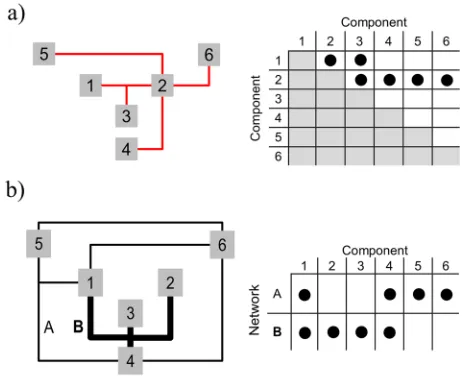
An example of a connection scheme for a number of compo-nents is presented in Fig.9. The fixed (prespecified) order connec-tions between the pairs of six components are shown in Fig.9(a). Where component 1 is shown with a line to 2 and 3 in this exam-ple, it means that 1 is connected to 2, 1 is connected to 3, and 3 is connected to 2 (not 1 is connected to 2 and 3), as only pairs are possible. The networks consisting of components that can be con-nected in any order are shown in Fig.9(b)(for example, a set of servos connected in a network with the power source). In this figure, the lines between the components show the possible connections between each pair of components. This flexible order connection problem is an example of the well-known traveling salesman problem (TSP).

The approach adopted for this study can outlined as:

(1) Identify the shortest routes between all pairs of components defined by the fixed order connection specification. (2) For each network of the flexible order connection, generate

a distance matrix by identifying the shortest routes between all possible component-pair combinations (for n compo-nents there aren_C

2pairs, wherenCm¼n!=½ðnmÞ!m!. (3) Solve the equivalent TSP combinatorial problems by

utiliz-ing the aforementioned distance matrix to identify the com-ponent connection order within each network.

Sections 2.3.1–2.3.4 will elaborate on the above outlined key aspects of the routing strategy, specifically; shortest path identifi-cation using the accurate and approximate methods, solving the TSP problem with metaheuristics, and computational strategies for increased efficiency.

2.3.1 Shortest Path Identification: Accurate Method.The problem of computing the shortest path of a graph is an interesting one and since the paper from 1959 detailing Dijkstra’s algorithm [23], which solves the single-source shortest path problem for a graph (with non-negative edge path costs), a considerable effort has been made by researchers to build on this technique, primarily due to its applicability to a wide range of problems.

One example of this is the fast marching (FM) method which uses approximate gradient values to compute the discrete solution Fig. 8 Identification of the component orientation vectors

to the eikonal equation, which is a nonlinear partial differential equation encountered in problems of wave propagation [24]. The FM method allows the efficient computation of (stable) solutions for a large class of continuous problems, while retaining the idea of a one-pass algorithm as is the case in Dijkstra’s algorithm and for that reason it was the choice of algorithm for this work. To identify the shortest route between any two considered compo-nents, a MATLABimplementation of FM [25] was used. The key stages of this method are:

(1) Generate a speed image,I(containing the marching speed at any given point in the structure)

I¼aMþ1 (4)

whereMis the material matrix corresponding to the struc-ture (entries are 1 for solid and 0 for void) andais a scaling factor (the value of 50 was chosen for this as doing so suffi-ciently biases the routes so that they are constrained to the solid region).

(2) Obtain the distance map,D, of the speed image,I, using the FM implementation

D¼fFMðIÞ (5)

(3) Generate a gradient map,G, by numerically computing the gradients on the obtained distance map [26].

(4) Use a steepest descent algorithm onGto identify the short-est path.

2.3.2 Shortest Path Identification: Approximate Method.As an alternative to the accurate method for finding the shortest path, an approximate method can be used which uses the geometric in-formation of the part contained in a medial axis. The effectiveness of this method at replacing the accurate method can be exploited in two instances. First, the geometry that routes is passing through, for example, thin members; and second, for cases where lower accuracy can be tolerated, such as when identifying the shortest routes between all possible component-pair combinations in a network to generate the distance matrix. The tradeoff between efficiency and accuracy is investigated in test case 2 in Sec.3.2. The approximate approach is described by the following steps:

(1) Obtain the medial axis of the part.

(2) Compute the length of each medial axis member (i.e., branch point to branch point).

(3) Identify the link and the points on it, which are nearest to the placement location. Find the distance from the above mentioned points to the branch points of the link they lie on (see Fig.10).

(4) Develop a graph (network) representing the path finding problem.

(5) Solve the graph problem using Dijkstra’s algorithm [23].

2.3.3 Shortest Network Problem: Solving With Metaheuristics. It is only practical to find the exact solution for a TSP through exhaustive search when the problem size is small, because the run time for this approach lies within a polynomial factor of O(n!), wherenis the number of components in a network (note: O(n) implies that the algorithm has order ofntime complexity). There-fore, a more efficient approach, ACO [27] is used here to solve the TSP.

The ACO technique is a metaphorical representation of the colonial foraging behavior of ants. An artificial ant in ACO is a stochastic constructive procedure that incrementally builds a solution by adding opportunely defined solution components (pheromones) to a partial solution under construction [28]. The colony’s ability to find better solutions is enhanced by incorporat-ing an evaporation coefficient that promotes the exploration of new solutions without being overconstrained by past decisions [29]. The two key aspects of the ACO implementation are discussed below:

First, the stochastic nature of the algorithm comes from the probabilistically governed random decision that an ant makes to move from the current component location to the next unvisited one. The underlying probabilities are computed as

Pk_ijðtÞ ¼aijðtÞ .X

l

ailðtÞ (6)

wherePk_ijðtÞis the probability of moving from theith to the jth component location by thekth ant in thetth iteration, and the term aijðtÞis the functional composition of the pheromone trail,s, and the local heuristic,g, often expressed as

aijðtÞ ¼ sijðtÞ

a

ðg_ijðtÞÞb (7)

where the heuristic information,g_ij, is the inverse of the distance between the two component locations, and the two parametersa

(set to 1) andb(set to 2) determine the relative influence of phero-mone trail and heuristic information, respectively.

The second key aspect relates to the update of the pheromone information, which is done after the completion of a colonial search using

sijðtþ1Þ ¼ ð1qÞ sijðtÞ þ Xm

k¼1

Dsk

ij (8)

whereqis the evaporation coefficient (set as 0.1),mis the total number of ants selected for pheromone deposition from the colony (only ants that perform better than the average of the colony are chosen), and the Dsk

ij term represents the amount of pheromone thekth ant deposits on the path (i,j) defined as

Dsk_ij¼ 1=Lkð Þt if pathði;jÞis used by antk

0 otherwise

(9)

whereLk_{is the length of thekth ant’s tour. It is of note that in} gen-eral, paths that are used by many ants and that are contained in

Fig. 10 Approximate routing method: shortest path identifica-tion based on the medial axis. Distances between points are represented by double ended arrows.

shorter tours will receive more pheromone, and therefore are also more likely to be chosen in future iterations of the algorithm.

To enable an automated TSP solver, both the number of ants and colonial iterations for ACO were set to four times the number of components in a network. Furthermore, a convergence toler-ance of 1106was used.

2.3.4 Computational Strategy: Clustering Method for Increased Efficiency.With regard to solving the shortest network problem itself, the authors propose restating the problem so that it can (where possible) be decomposed into smaller TSPs [30]. Doing so offers computational leverage that is proportional to the extent of decomposition. This is illustrated in Fig.11where, after restating the original TSP into three smaller ones, the computa-tional effort can be reduced from

ðS1þS2þS3Þ_C

2toðS1C2þS2C2þS3C2Þ (10)

In general, we can express this leverage as P

Si_C

2

. X_Si

C2 (11)

which, for simplicity sake, can be understood as

1þ X

i6¼j

SiSjX

i¼j SiSj

!

(12)

with the assumption that n_C

2n2=2. It is noteworthy that this

decomposition is possible only when the component locations are clustered together, and it is this clustering/grouping that allows greatest benefit from this strategy.

3

Simulations and Results

In order to effectively assess the proposed placement and rout-ing strategy, three test cases are considered in this section. These test cases evaluate the strategy’s various key elements progres-sively, from a fundamental to an applied standpoint. Test case 1

aims to test the accuracy and appropriateness of the underlying fundamental principles on which the method is based. Test case 2 explores the efficacy of the proposed approximate routing method with a set of examples. Finally, test case 3 considers a complex 3D problem from an application standpoint to assess the effective-ness of the proposed placement and routing strategy.

3.1 Test Case 1: Accuracy of Underlying Principles.Test case 1 aims to test the accuracy of the underlying fundamental principles on which the proposed placement and routing strategy is based, and is comprised of the following three subcases:

(a) component placement and orientation control (b) shortest path finding ability of FM

(c) the ability of ACO to solve the shortest network problem (i.e., TSP)

The geometry shown in Fig.12(a)will be used to assess the pro-posed placement philosophy. Here, we have three components that are placed at specified locations. As explained in Sec.2.2.3, com-ponents are oriented along the dominant local direction vector amongst those that lie within a neighborhood (defined by circles drawn around the components and having radii of 1.5 times the dis-tance to closest link). For component 1, there is more than one member that lies within the neighborhood, and therefore, the domi-nant local direction vector needs to be identified. In this case, the dominant local direction vector is the one that is more closely aligned with other local direction vectors (see Sec. 2.2.3 for details). Consequently, this results in what would be considered a visually more appropriate solution. On the contrary, in the cases of components 2 and 3, where the neighborhood encompasses only one member, these components are aligned with their local direc-tion vectors, which again would be considered a visually appropri-ate solution.

A plate with a hole in its center (see Fig.12(b)) is used for test case 1b, i.e., to assess the shortest path finding ability of the FM implementation. The primary reason for this choice is the existence of a well-defined analytical solution, consisting of the appropriate tangent segment from the start point, appropriate tangent segment from the end point, and the minor circular segment between the tangent locations. From Fig.12(b), it can be observed that the nu-merical solution obtained with the FM implementation only slightly deviates from the true shortest path, and therefore provides a reasonably high level of accuracy that is fit for our purpose.

The robustness of ACO to solve combinatorial problems is well documented [27]. In addition to this, benchmarking of the

Fig. 12 Test case 1—assessing: (a) component placement and orientation control and (b) shortest path finding ability of the accurate method between two points

in-house ACO code was carried out using standard TSPs taken from Refs. [31,32], for which the minimum tour lengths were known and the chosen ACO parameters (described in Sec.2.3.3) enabled convergence to the known solutions.

3.2 Test Case 2: Comparison of Routing Approaches.Test case 2 compares the two shortest path identification approaches, specifically, the accurate method and the approximate method, on two example cases:

(a) a 2D “X”-shaped part, and (b) the 3D geometry of Fig.5(a).

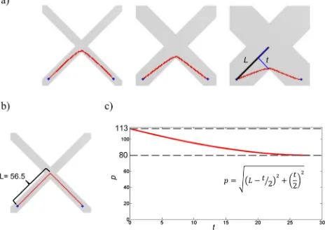
The experiment of test case 2a was performed on an X-shaped part (see Fig. 13), which was selected as it has an unchanging medial axis (when subject to changes in the member thickness). This enabled the relative range of deviation likely to be encoun-tered in an applied problem to be included.

The path length, p, obtained using the accurate method was seen to change according to

p¼

ffiffiffiffiffiffiffiffiffiffiffiffiffiffiffiffiffiffiffiffiffiffiffiffiffiffiffiffiffiffiffiffiffiffiffiffi

ðLt=2Þ2þ ðt=2Þ2

q

(13)

whereLis the length of half of the medial axis link andtis half the member width. In contrast, the path length for the approximate method remained unchanged as the medial axis was unaltered. This resulted in a relative range of deviation in length of [0,ðpffiffiffi21Þ]100%.

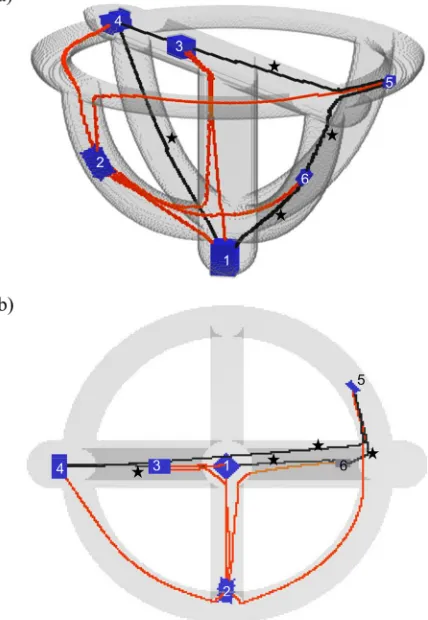
Test case 2b aims to better understand the implications of using the two different routing approaches on a 3D geometry. Here, six internal components connected in a cyclic pattern within the geometry are considered. The two key aspects of interest in this experiment are: accuracy of the result (i.e., path lengths) and its efficiency (i.e., computational expense). Figure14shows that, in general, the paths take an approximately similar course for both the accurate and approximate methods, however, occasionally there can be significant differences in routes, as is observed in the

case of path “4,” which nevertheless have very similar path lengths (see Tables1and2).

Table1reports the accuracy of the results, i.e., the error in the path lengths when employing the approximate routing method. It is observed that the approximate method overestimates path length by about 20% on average. Table2reports the time required to identify routes using the two routing methods. It is observed that the approximate method is almost 25faster than the accu-rate method. Section4discusses how and when the two routing approaches could be incorporated within the placement and routing strategy.

3.3 Test Case 3: Assessment of Placement and Routing Capabilities.Test case 3 applies the component connection scheme of Fig. 9 (excluding network “B”) on the geometry of Fig. 5(a) to assess the effectiveness of the proposed placement Fig. 14 Results for test case 2b—shortest paths/routes on a

3D geometry when employing: (a) the accurate method and (b) the approximate method based on the medial axis

Table 1 Path lengths (in voxel length scale) when employing the accurate and approximate routing methods

Path 1 Path 2 Path 3 Path 4 Path 5 Path 6

FM method results 49 94 27 117 53 42

Approximate method results 60 117 32 126 66 53

Error (in %) 22.5 24.5 18.5 7.7 24.5 26

Table 2 Computational time (in seconds) for path identification when using the accurate and approximate routing methods

Path 1 Path 2 Path 3 Path 4 Path 5 Path 6

FM method results 1.548 1.535 1.562 1.551 1.567 1.566

Approximate method results 0.063 0.063 0.060 0.060 0.063 0.060

(Accurate (time)/approx. (time)) 24.5 24.5 26 26 25 26

and routing strategy from a more realistic application standpoint. This test case includes 3D orientation control and both fixed and flexible order routing. The list of component placement locations is populated by adopting the previously described unconstrained (geometry based) approach (refer to Fig.6of Sec.2.2), and the shortest paths were identified using the FM method.

Figures15(a)and15(b)show the advanced routing features for the fixed and flexible order connections on the considered 3D ge-ometry. Paths shown in red represent the fixed order connectivity while the paths in black (and tagged with a star$_{) represent the}

flexible order connectivity. Due to the unique geometry under consideration, it can be observed that all the paths are composed of, in some combination, the following segment types: straight lines, circular arcs, and arcs of varying curvature. Additionally, components can be seen to be aligned with either the members’ local tangent or, alternatively, strongly influenced by the members in its vicinity (refer to Sec.2.2.3for details).

4

Discussion

To recap, the ultimate aim of this work is to outline and formal-ize a set of techniques/methods that aid the design of a multifunc-tional component. The specific objectives are:

(1) to devise a suitable framework to enable the design of mul-tifunctional parts

(2) to devise a suitable strategy to determine suitable locations for the internal components

(3) to devise a suitable strategy to connect the internal compo-nents into a circuit

The presented test cases provide an illustration of the workings of the proposed placement and routing method and demonstrate that the presented set of techniques are effective at exploiting the true-3D design freedom of PCVs.

The implemented strategy currently tackles the procedure of placement and routing in a sequential fashion. Currently, determi-nation of a location for a particular component does not consider the location of adjacent components (apart from ensuring no over-lapping components and that a minimum spacing constraint is observed). Placement considering other components may be required for reasons such as heat dissipation, latency or timing requirements, or just from an overall circuit efficiency require-ment. It is clear that the placement of components has a large effect on the overall circuit efficiency, and so the coupling strat-egy presented in the overall framework of Fig.2is required to take account of these dependencies. This can be achieved through a combinatorial optimization scheme but as was mentioned in the introduction, this is a computationally intensive task and so heuristic strategies may be more suitable.

The issue of timing requirements, an application-driven design constraint of Fig.2, can be addressed using the current strategy, although limited to one direction only, that is, to increase the length of connections, rather than decrease them. This can be achieved with a mapping of predefined route lengthening patterns (which could be in 3D) to the existing shortest paths (Fig.16(d)). This works in the same principle as mapping of bundled connec-tions between groups of components following clustering (Fig.16(c)). The same approach can also be used to control the conductivity of particular connections between components by varying their diameters or thicknesses once the relationship between dimensions and conductivity for a particular material is understood (Fig.16(b)). However, this just enables a specific per-formance criteria be met, rather than allowing the overall circuit to be optimized. To this end, it is proposed that the clustering method be extended to also include grouping by which compo-nents are connected as well as which compocompo-nents are located near to each other. This will allow for an iterative adjustment of the component placement to improve the overall circuit efficiency.

The component placement strategy can be extended to include more advanced features such as to handle problems where

maximum component packing efficiency is a requirement, such as for very compact systems; checking whether the component fits within the part at the placed location by ensuring that the majority of the components’ surface voxels lie within the part. Such exten-sions would improve the robustness of the proposed placement strategy.

Regarding routing, the described methods: accurate and approx-imate have been found to be effective at finding shortest routes between components. This strategy assumes that minimum length is desired, from a circuit efficiency and conductive material usage point of view. The accurate approach allows for voxel-by-voxel control of the routed path, which provides a greater level of opti-mality than the approximate approach for most structures. Their results tend to converge for structures that consist of solely slender members such as a lattice structure, where the routes taken match with the medial axis (which is used to calculate approximate paths). However, the reduction in computational burden through the use of the approximate method is dramatic and is especially useful: (a) when generating the distance matrix (by computing the shortest routes between all possible component-pair combina-tions), which is required for solving the shortest network problem for components without a prespecified connection order, (b) when considering the initial stage of the coupled optimization problem (“structure and internal system coupling strategy” of Fig. 2), where an approximate representation of the system is sufficient as the structural topology is still evolving, and (c) when tackling very large problems, where the computational resources available are insufficient for the accurate routing approach. The current implementation allows for both accurate and approximate methods to be used together.

Considering connection constraints, as well as the aforemen-tioned mapping method for route lengthening and diameter modi-fication, a route spacing constraint was implemented which ensured control of interference between adjacent connections. The routing also avoided obstacles within the geometry such as other internal components, other routed connections, and void regions. While the order in which the connections are made has a large effect on the overall result in 2D (due to route blocking), in 3D this is much less of a problem, apart from for thin geometric mem-bers that may not be able to accommodate multiple routes. To accommodate these cases, geometry modification methods are under consideration to thicken up regions of the part where benefi-cial to the overall system design. This would fall into the overall framework in the structure and internal system coupling strategy.

could be extended to other manufacturing methods, such as extrusion-based and hybrid manufacturing processes (e.g., embed-ding off-the-shelf components within an AM part) with different manufacturing constraints. Placement of components in such a hybrid process can be handled by utilizing the “design constraints,” specifically, the “geometric constraints” of Fig. 2 (see Sec.2.1.3for details). In this case, for instance, the compo-nents’ orientation could be restricted to the x–y plane so as to keep the components normal aligned to the parts’ build orienta-tion, making embedding possible.

It is of note that the proposed overall design framework of Fig. 2is modular in nature. Although in this work, the authors have focused on achieving multifunctionality via the electrical systems route, the general method can be readily extended to other functionality, such as optical, thermal, or fluid based. With any chosen route to multifunctionality, appropriate design constraints and suitable system enabling techniques can be selected and it is this problem independent aspect of the proposed framework that makes it modular.

5

Conclusions

This paper has proposed a framework for the design of PCVs, which are AM multimaterial parts with embedded functional systems. The primary objective of this work was to exploit the true-3D design freedoms of the MFAM paradigm and to this end, placement and routing techniques/methods that aid in the design of PCVs were outlined and formalized. The focus of the work pre-sented is on the placement and routing strategies which are two of the fundamental strands of the framework.

The proposed placement approach capitalizes on both the per-formance and geometric aspects of the considered part. A medial axis-based orientation scheme was proposed for appropriate compo-nent alignment. With regard to the routing (path length minimization problem), an FM method in conjunction with an ACO algorithm was used. The inclusion of approximate strategies, specifically, the ap-proximate routing method and the decomposition of the shortest net-work problem based on clustering are shown to greatly enhance the efficiency of the automated placement and routing strategy.

The proposed methods were evaluated progressively from a fundamental to an applied standpoint on numerous test cases. The results of which clearly demonstrated the appropriateness and effectiveness of the presented set of techniques for PCV design. The capability of the method allows the exploitation of the manu-facturing capability under development within the AM commu-nity to produce 3D internal systems within complex structures.

As this work has not focused on the structure and internal sys-tem coupling strategy within the framework, the geometry of all example parts, within which the internal system is placed, is fixed. The primary next step of this work is to devise, evaluate, and for-malize suitable coupling strategies; specifically, the coupling between placement and routing, and the coupling between the structural optimization and the placement and routing to realize the coherent design procedure of the MFAM design framework.

Acknowledgment

The authors would like to thank the UK Engineering and Physi-cal Sciences Research Council (EPSRC) for funding this work (Grant No. EP/I033335/2).

References

[1] Lopes, A. J., MacDonald, E., and Wicker, R. B., 2012, “Integrating Stereoli-thography and Direct Print Technologies for 3D Structural Electronics Fabrication,”Rapid Prototype J.,18(2), pp. 129–143.

[2] Vidimce, K., Wang, S.-P., Ragan-Kelley, J., and Matusik, W., 2013, “OpenFab: A Programmable Pipeline for Multi-Material Fabrication,” ACM Trans. Graphics,32(4), pp. 1–11.

[3] Ponche, R., Hascoet, J. Y., Kerbrat, O., and Mognol, P., 2012, “A New Global Approach to Design for Additive Manufacturing,”Virtual Phys. Prototyping, 7(2), pp. 93–105.

[4] Amos, M., Matthew, C.-W., and Wimhurst, S., 2013, “3D Printed Prosthetic Arm,” University of Nottingham, Nottingham, UK.

[5] Abboud, N., Gr€otschel, M., and Koch, T., 2007, “Mathematical Methods for Physical Layout of Printed Circuit Boards: An Overview,”OR Spectrum,30(3), pp. 453–468.

[6] Chan, T. F., Cong, J., Shinnerl, J. R., Sze, K., and Xie, M., 2006, “Multiscale Optimization in VLSI Physical Design Automation,”Multiscale Optimization Methods and Applications(Nonconvex Optimization and Its Applications, Vol. 82), Springer-Verlag, New York, pp. 1–67.

[7] Areibi, S., and Yang, Z., 2004, “Effective Memetic Algorithms for VLSI Design¼Genetic AlgorithmsþLocal SearchþMulti-Level Clustering,”Evol. Comput.,12(3), pp. 327–353.

[8] Park, J.-H., and Storch, R. L., 2002, “Pipe-Routing Algorithm Development: Case Study of a Ship Engine Room Design,” Expert Syst. Appl., 23(3), pp. 299–309.

[9] Ma, X., Iida, K., Xie, M., Nishino, J., Odaka, T., and Ogura, H., 2006, “A Genetic Algorithm for the Optimization of Cable Routing,”Syst. Comput. Jpn.,37(7), pp. 61–71.

[10] Thantulage, G. I. F., 2009, “Ant Colony Optimization Based Simulation of 3D Automatic Hose/Pipe Routing,” Ph.D. thesis, Brunel University, Middlesex, UK.

[11] Velden, C., Bil, C., Yu, X., and Smith, A., 2007, “An Intelligent System for Automatic Layout Routing in Aerospace Design,”Innovations Syst. Software Eng.,3(2), pp. 117–128.

[12] Guo, H. Y., Zhang, L., Zhang, L. L., and Zhou, J. X., 2004, “Optimal Placement of Sensors for Structural Health Monitoring Using Improved Genetic Algorithms,”Smart Mater. Struct.,13(3), pp. 528–534.

[13] Flynn, E. B., and Todd, M. D., 2010, “A Bayesian Approach to Optimal Sensor Placement for Structural Health Monitoring With Application to Active Sensing,”Mech. Syst. Signal Process.,24(4), pp. 891–903.

[14] Beyne, E., 2006, “3D System Integration Technologies,” International Sympo-sium on VLSI Technology, Systems, and Applications, Hsinchu, Taiwan, Apr. 24–26, pp. 1–9.

[15] Brackett, D., Panesar, A., Ashcroft, I., Wildman, R., and Hague, R., 2013, “An Optimization Based Design Framework for Multi-Functional 3D Printing,” 24th Annual International Solid Freeform Fabrication Symposium, Austin, TX, Aug. 12–14, pp. 592–605.

[16] Panesar, A., Brackett, D., Ashcroft, I., Wildman, R., and Hague, R., 2014, “Design Optimization Strategy for Multifunctional 3D Printing,” 25th International Solid Freeform Fabrication Symposium, Austin, TX, Aug. 4–6, pp. 1179–1193.

[17] Bendsoe, M. P., and Sigmund, O., 2003,Topology Optimization: Theory, Methods, and Applications, Springer-Verlag, Berlin.

[18] Huang, X., and Xie, Y. M., 2010,Evolutionary Topology Optimization of Continuum Structures, 1st ed., Wiley Publication, John Wiley & Sons Ltd, Chichester, UK.

[19] Aremu, A., Ashcroft, I., Wildman, R., Hague, R., Tuck, C., and Brackett, D., 2013, “The Effects of Bidirectional Evolutionary Structural Optimization Parameters on an Industrial Designed Component for Additive Manufacture,”

Proc. Inst. Mech. Eng., Part B,227(6), pp. 794–807.

[20] Abdi, M., Wildman, R., and Ashcroft, I., 2013, “Evolutionary Topology Optimization Using the Extended Finite Element Method and Isolines,”Eng. Optim.,46(5), pp. 628–647.

[21] Lee, T., and Kashyap, R., 1994, “Building Skeleton Models Via 3-D Medial Surface Axis Thinning Algorithms,”Graphical Models Image Process.,56(6), pp. 462–478.

[22] Kerschnitzki, M., Kollmannsberger, P., Burghammer, M., Duda, G. N., Wein-kamer, R., Wagermaier, W., and Fratzl, P., 2013, “Architecture of the Osteocyte Network Correlates With Bone Material Quality,”J. Bone Miner. Res.,28(8), pp. 1837–1845.

[23] Dijkstra, E. W., 1959, “A Note on Two Problems in Connexion With Graphs,”

Numer. Math.,1(1), pp. 269–271.

[24] Sethian, J. A., 1996, “A Fast Marching Level Set Method for Monotonically Advancing Fronts,”Proc. Natl. Acad. Sci. U. S. A.,93(4), pp. 1591–1595. [25] Peyre, G., 2009, “FM Code,” http://www.mathworks.co.uk/matlabcentral/

fileexchange/6110-toolbox-fast-marching

[26] Mathworks, 2013, “MATLAB R2013a,” Natick, MA.

[27] Dorigo, M., and St€utzle, T., 2004, Ant Colony Optimization, The MIT Press, Cambridge, MA.

[28] Dorigo, M., Maniezzo, V., and Colorni, A., 1996, “Ant System: Optimization by a Colony of Cooperating Agents,”IEEE Trans. Syst., Man, Cybern., Part B, 26(1), pp. 29–41.

[29] Dorigo, M., Di Caro, G., and Gambardella, L. M., 1999, “Ant Algorithms for Discrete Optimization,”Artif. Life,5(2), pp. 137–172.

[30] Lian, L., and Castelain, E., 2009, “A Decomposition-Based Heuristic Approach to Solve General Delivery Problem,” World Congress on Engineering and Computer Science, San Francisco, CA, Oct. 20–22, pp. 1078–1082.

[31] Burkardt, J., “Data for the Traveling Salesperson Problem,” http://people. sc.fsu.edu/jburkardt/datasets/tsp/tsp.html