http://wrap.warwick.ac.uk/
Original citation:
Ferraz-Leite, S., Ortner, Christoph and Praetorius, D.. (2010) Convergence of simple
adaptive Galerkin schemes based on h − h/2 error estimators. Numerische Mathematik,
Vol.116 (No.2). pp. 291-316.
Permanent WRAP url:
http://wrap.warwick.ac.uk/48591
Copyright and reuse:
The Warwick Research Archive Portal (WRAP) makes this work of researchers of the
University of Warwick available open access under the following conditions.
This article is made available under the Creative Commons Attribution- 3.0 Unported
(CC BY 3.0) license and may be reused according to the conditions of the license. For
more details see
http://creativecommons.org/licenses/by/3.0/
A note on versions:
The version presented in WRAP is the published version, or, version of record, and may
be cited as it appears here.
Numer. Math. (2010) 116:291–316 DOI 10.1007/s00211-010-0292-9
Numerische
Mathematik
Convergence of simple adaptive Galerkin schemes
based on h
−
h
/
2 error estimators
S. Ferraz-Leite · C. Ortner · D. Praetorius
Received: 9 April 2009 / Revised: 26 December 2009 / Published online: 30 March 2010 © The Author(s) 2010. This article is published with open access at Springerlink.com
Abstract We discuss several adaptive mesh-refinement strategies based on(h− h/2)-error estimation. This class of adaptive methods is particularly popular in practise since it is problem independent and requires virtually no implementational overhead. We prove that, under the saturation assumption, these adaptive algorithms are con-vergent. Our framework applies not only to finite element methods, but also yields a first convergence proof for adaptive boundary element schemes. For a finite element model problem, we extend the proposed adaptive scheme and prove convergence even if the saturation assumption fails to hold in general.
Mathematics Subject Classification (2000) 65N30·65N38·65N50·65N12
1 Introduction
Introductory remarks
LetHbe a real Hilbert space with scalar product·,·and associated energy norm ||| · |||. Given a right-hand side F ∈ H∗, we aim at a numerical approximation of the unique solution u∈Hof
u, v =F(v) for allv∈H. (1)
S. Ferraz-Leite·D. Praetorius (
B
)Institute for Analysis and Scientific Computing, Vienna University of Technology, Wiedner Hauptstrasse 8-10, 1040 Vienna, Austria
e-mail: [email protected] S. Ferraz-Leite
e-mail: [email protected]
C. Ortner
To that end, let X be a finite-dimensional subspace ofH, which in many applica-tions is based on a triangulationT of some physical domain. Let u ∈ X be the corresponding Galerkin solution, obtained by solving the finite-dimensional linear system
u, v =F(v) for allv∈ X. (2)
Throughout, the index∈ N0:= {0,1,2, . . .}denotes the step of an adaptive algo-rithm, and associated quantities are discrete and numerically computable.
Whereas uniform refinement of the meshesTusually leads to convergence u→u
as→ ∞, this cannot be expected, in general, if the meshes are only refined locally by means of an adaptive algorithm. We say that an adaptive mesh-refining algorithm is convergent if, and only if, u → u as → ∞. In this sense, convergence of an adaptive algorithm has first been proven by Dörfler [12], where also the marking cri-terion (7) used in Algorithm1 below is introduced. The latter work considered the residual error estimator for a P1-finite element discretization of the Poisson problem, and it is assumed that data oscillations on the initial mesh are sufficiently small. In [19], the resolution of the data oscillations is included into the adaptive algorithm. The convergence analysis is based on reliability and the so-called discrete local efficiency of the residual error estimator, which relies on an interior node property for the local mesh-refinement. The main idea of the convergence proof then is to show that the error is contractive up to the data oscillations. Cascon et al. [10] recently presented a new convergence proof under weaker conditions. They showed that a weighted sum of error and error estimator satisfies a contraction property without requiring (discrete local) efficiency of the estimator. In all of the cited works [10,12,19], however, the focus was only on residual-based error estimators for conforming finite element schemes.
(h−h/2)-Error estimation and adaptive algorithm
In contrast to the preceding works, we study the(h−h/2)-error estimation strategy which is a well-known technique for the a posteriori estimation of the error in the energy norm|||u−u|||; see [16] in the context of ordinary differential equations, and the works of Bank [3–5] or the monograph [1, Chapter 5] in the context of the finite element method. LetTbe a uniform refinement ofTand let X be the associated finite-dimensional subspace ofH with corresponding Galerkin solutionu ∈ X. Then, the(h−h/2)-error estimator
η := |||u−u||| (3)
is a computable quantity [11] which can be used to estimate the error|||u−u|||. By use of the Galerkin orthogonality property it is easy to see that
where the upper bound is equivalent to the so-called saturation assumption
|||u−u||| ≤Csat|||u−u||| with some uniform constant Csat∈(0,1), (5)
see e.g. [1, Theorem 5.1]. We remark that the saturation assumption dates back to the early work [5], but may fail to hold in general [6,13].
To steer an adaptive mesh-refinement, we additionally assume that(T)is a com-putable quantity which (at least heuristically) measures the local error between the exact solution u and a discrete solution u∈ Xon an element T ∈T. To link these so-called refinement indicators withη, we assume that
C1−1η≤ :=
⎛
⎝
T∈T
(T)2 ⎞ ⎠
1/2
≤C2η for all∈N, (6)
with-independent constants C1,C2>0. The adaptive mesh-refining algorithm then
reads as follows:
Algorithm 1 Let an initial triangulationT0with associated discrete space X0and an adaptivity parameterθ∈(0,1)be given. For=0,1,2, . . .do the following:
(a) Compute the discrete solution u∈ X.
(b) Compute the refinement indicators(T)for all T ∈T.
(c) Stop if uis sufficiently accurate (e.g.,resp.ηis sufficiently small). (d) Otherwise, choose a setM⊆Tof marked elements such that
θ
T∈T
(T)2≤
T∈M
(T)2. (7)
(e) Refine at least the marked elements T ∈M, generate a new meshT+1and an associated discrete space X+1, increase the counter→+1, and go to (a).
Outline
In the present paper, we adapt the arguments from [10] to(h−h/2)-based error estima-tion techniques and investigate the convergence of Algorithm1steered by(h−h/2) -based refinement indicators. In Sect.2, linear finite elements for the numerical solution of the 2D Poisson problem are studied. We consider the indicators
μ(T):= ∇u−(∇u)L2(T)
and μ(T):= ∇(u−Iu)L2(T) for T ∈T, (8)
that Algorithm1, steered by =μ, and for any choice ofθ ∈ (0,1), guarantees the contraction property
+1≤κ with := |||u−u|||2+ |||u−u|||2+γ 2 (9)
and with appropriate constantsκ, γ ∈ (0,1). In particular, the adaptive algorithm is convergent (Theorem4). We also consider Algorithm1steered by =μ, where convergence limu =u follows for arbitraryθ ∈(0,1), but a contraction property (9) is only proven forθsufficiently large (Theorem5).
In [13], it has been observed that small data oscillations imply the saturation assump-tion. In Sect.2.6, we incorporate this observation in the convergence analysis in the sense that we enhance the refinement indicatorsμ(T)andμ(T)by the local data oscillations osc(T)defined in (40) below. Using these combined refinement indica-tors, e.g.2 =μ2+osc2, the data is adaptively resolved by Algorithm1, and we obtain convergence u → u as→ ∞, independently of the saturation assumption (Theorem6).
In addition to the adaptive finite element method, our arguments also apply to bound-ary integral formulations discussed in Sect.3. As model example serves the elliptic integral formulation of the Laplace problem with Dirichlet boundary conditions in 2D and 3D. We use the(h−h/2)-based error indicators
μ(T):= h1/2(u−u)
L2(T) and μ(T):=
h1/2(u
−u)
L2(T) (10)
from [14] to steer the adaptive mesh-refinement. Under the saturation assumption (5), we prove that the associated error quantity satisfies the contraction property (9) for both, theμ-steered and theμ-steered adaptive algorithm (Theorem7–8). This yields a first convergence proof for the adaptive boundary element method.
Finally, in Sect.4, numerical experiments for both, finite element and boundary element methods, are performed. The results verify our analysis empirically and sug-gest the validity of the saturation assumption even in the context of boundary element methods.
2 Finite element method
2.1 Model problem
We consider the elliptic model problem
−u = f in,
u =0 onD, (11)
∂nu =g onN.
Here,is a bounded Lipschitz domain inR2with polygonal boundary. The boundary
=D∪Nas well asD∩N = ∅. Moreover, we assume thatDhas positive
surface measure|D| > 0 so that (11) admits a unique weak solution. The energy
scalar product of the weak formulation of (11) reads
u, v :=
∇u· ∇vdx for all u, v∈H=u ∈H1() : u|D =0
, (12)
and the right-hand side is given by
F(v)=
fvdx+
N
gvds, (13)
where ds denotes integration along the boundary. In particular, the energy norm reads |||v||| = ∇vL2(). We consider the lowest-order Galerkin scheme, whereT is a regular triangulation ofin the sense of Ciarlet and where X = v ∈ S1(T) :
v|D =0
withS1(T)=v∈C() : ∀T ∈T v|T is affine
.
To fix notation,Ndenotes the set of nodes ofT, andEdenotes the set of edges of T. Moreover,EN, denotes the set of all edges, which belong to the Neumann
boundaryN. The local mesh-width h∈ L∞()is defined by h(x)=diam(T)for T ∈Tand x ∈interior(T). Moreover, h(x)=diam(E)if x belongs to the relative interior of an edge E ∈ E. Finally,Pp(T)denotes the space of all T-piecewise polynomials of total degree≤ p, andS1(T)=P1(T)∩C().
2.2 Mesh-refinement
The essential point in the analysis below is that all sons T ∈T+1of a marked ele-ment T ∈Malso belong to the uniform refinementTofT. We therefore generate both meshesT+1andTby the same refinement strategy with respect to the marked elementsMandM:=T, respectively.
Our mesh-refinement is a variant of the newest vertex bisection algorithm (cf. Fig. 1), using an edge-based formulation: For a marked element T , we mark all of is edges for refinement. To avoid hanging nodes and to ensure regularity of the refined triangulation, we then proceed recursively: If any edge of an element T is marked for refinement, we also mark its reference edge. This recursion necessarily terminates after finitely many steps with the result that, for each element in which at least one edge is marked for refinement, the reference edge is marked as well. We then proceed with the refinement rules for newest vertex bisection shown in Fig.2.
For further details on newest vertex bisection, the reader is referred to [23, Chapter 4] or the original works [2,17,21]. We stress that all generated meshes are uniformly shape regular, see Fig.3.
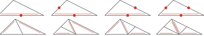
Fig. 1 For each triangle T ∈T, there is one reference edge, indicated by the doubleli ne (le f t). Bisection of T is achieved by halving the reference edge, where its midpoint becomes a new node. The reference edges of the son triangles are opposite to this newest vertex (le f t-mi ddle). Further steps of newest vertex bisection lead to steps, which are denoted by bisec3(T)and bisec5(T), respectively (r ight-mi ddle,r ight)
Fig. 2 Refinement by newest vertex bisection: We consider one triangle T and assume that certain edges, but at least the reference edge, are marked for refinement (top). After refinement, the element is split into 2, 3, or 4 son triangles, respectively (bottom). Throughout, the reference edges are indicated by a doubleli ne
Fig. 3 Refinement by newest vertex bisection only leads to finitely many interior angles for the family of all possible triangulations obtained by arbitrary newest vertex bisections. To see this, we start from a macro element (le f t), where the bottom edge is the reference edge. Using iterated newest vertex bisection, one observes that only four similarity classes of triangles occur, which are indicated by the colour i ng. After three steps of bisections (r ight), no additional similarity class appears (color figure online)
We stress that refinement rules based on newest vertex bisection ensure the inclu-sions X ⊂ X+1 ⊆ X ⊂ X+1, which are crucial in our analysis. We remark that almost all mesh-refinement strategies will yield X⊂ X+1and X⊂X. However, the inclusions X+1⊂X⊂X+1may be violated. For instance, they fail in general for the popular red-green-blue refinement strategies [23, Chapter 04].
2.3 Saturation assumption
In [13], it is stated (without a proof) that the saturation assumption (5) holds for the homogeneous Dirichlet problem (11) withD = ∂, ifT is obtained by uniform
red-refinement ofTand if data oscillations are sufficiently small. Here, red-refine-ment means that each triangle T ∈Tis divided into four similar son triangles T1, . . . ,
T4∈T. The notion data oscillations is understood as
osc2 =
z∈N
h(f − f,z)
2
L2(ω
,z), (14)
whereω,z := T ∈ T : z ∈ T
is the patch of a node z with respect toT and where f,z := |ω,z|−1
[image:7.439.56.385.141.199.2] [image:7.439.58.388.253.285.2]
For N = ∅ and with bisec5 replacing red-refinement, an analogous result is already contained in [19], although not stated explicitly; compare Eq. (15) below and [19, Lemma 4.2]. For the mixed boundary value problem (11), we sketch the proof of the saturation assumption for the convenience of the reader.
Proposition 2 LetTbe obtained by uniform bisec5-refinement ofT, and let u∈ X
andu∈ Xbe the corresponding Galerkin solutions to (11). Then, there exists a
con-stantCsat∈(0,1)such that
|||u−u|||2≤Csat|||2 u−u|||2+osc2, (15)
where the data oscillations are defined by
osc2 = h(f −f)2L2()+ h 1/2
(g−g)
2
L2(
N)
. (16)
Here, denotes the L2-orthogonal projection ontoP0(T)andP0(EN,), respec-tively. Consequently, if
osc2 ≤λ|||u−u|||2, (17)
for some λ > 0 with C2
sat = Csat2 +λ < 1, then the saturation assumption (5) is
satisfied.
Sketch of Proof To prove (15), we consider the residual-based error estimator [23]
2
=
T∈T
(T)2
with local contributions
(T)2= hf2L2(T)+ h 1/2
[∂nu]
2
L2(∂T∩)+
h1/2
(g−∂nu)
2
L2(∂T∩
N) ,
where[·]denotes the jump over an interior edge E ∈E. It is well-known thatis reliable,
|||u−u||| ≤Crel. (18)
and locally efficient up to oscillation terms,
(T)2≤Ceff2
∇(u−u)2L2(ω
T)+ h(f −f)
2
L2(ω
T)
+ h1/2(g−g)
2
L2(∂T∩
N)
where ωT = {T} ∪ T ∈ T : T ∩T ∈ E
denotes the element patch of
T ∈T, cf. [23]. The proof of (19) goes back to Verfürth [22] and is obtained by use of appropriate bubble functions. First,
hfL2(T)∇u− ∇uL2(T)+ h(f −f)L2(T) (20)
follows by use of the element bubble bT ∈P3(T)∩H01(T). Second, for an interior edge E ∈ E, let E = T ∩Tand denote byωE =T ∪Tthe corresponding edge
patch. Then, by use of the edge bubble bE ∈P2({T,T})∩H01(ωE), one can prove
that
h1/2
[∂nu]
L2(E)∇u− ∇uL2(ωE)+ hfL2(ωE). (21)
Third, for a Neumann edge E∈EN,with corresponding element T ∈T, using again
the edge bubble bE ∈P2(T)with bE|∂T\E =0, one shows that h1/2
(g−∂nu)
L2(E)∇u−∇uL2(T)+hfL2(T) + h1/2(g−g)
L2(E). (22)
Using the triangle inequality and (20)–(22), one obtains (19).
In all of the three estimates (20)–(22), the term∇u on the right-hand side stems from
the weak form (1) applied with the properly weighted bubble functionsv∈ {bT,bE}.
It has already been observed by Dörfler [12] that one may use the hat functionv =
bE ∈ Xfor the midpoint of an edge E ∈Einstead of the edge bubble function. This
allows to use the Galerkin formulation (2) forXinstead of the continuous variational form (1) and leads to∇uinstead of∇u in (21)–(22). Finally, it was noticed in [19] that one may use the hat functionv=bT ∈Xwhich corresponds to the interior node
of bisec5(T)instead of the element bubble, cf. Fig.1. This leads to∇uinstead of∇u in (20). With these two observations, one can therefore use Verfürth’s proof to verify the local discrete efficiency
(T)2≤Ceff2
∇(u−u)2L2(ω
T)+ h(f −f)
2
L2(ω
T)
+ h1/2(g−g)
2
L2(∂T∩
N)
, (23)
for all T ∈T, even with the same constant as in (19). Summation over all elements
T ∈Tresults in
2
≤3C2eff
|||u−u|||2+osc2
(24)
Now, we are in a position to verify (15): The combination of (18) and (24) yields
|||u−u|||2≤Crel2 2≤3C2effCrel2
|||u−u|||2+osc2
.
With C :=3Ceff2 Crel2 , the Galerkin orthogonalities forXand X⊂Xprove
|||u−u|||2= |||u−u|||2− |||u−u|||2≤(C−1)|||u−u|||2+C osc2.
Thus, a further application of the Galerkin orthogonality yields
C|||u−u|||2≤(C−1)|||u−u|||2+C osc2
and concludes the proof withCsat2 =(C−1)/C.
2.4 Refinement indicators
In this section, we discuss the refinement indicators
μ(T)= ∇u−(∇u)L2(T) and μ(T)= ∇(u−Iu)L2(T), (25)
as well as
η(T)= ∇u− ∇uL2(T). (26)
Here, : L2()2 → P0(T)2 denotes the L2-orthogonal projection onto the T-piecewise constant fields, and I : C()→ X denotes the nodal interpolation operator. Sinceis even theT-piecewise orthogonal projection and∇u∈P0(T)2, it holds that
μ(T)≤μ(T) and μ(T)≤η(T) for all T ∈T. (27)
Together with the best approximation property of the Galerkin solution u∈ X, this provides the global estimates
μ= ∇u−(∇u)L2()≤η≤μ= ∇(u−Iu)L2(). (28)
The following proposition states the converse inequalities.
Proposition 3 There is a constant C3≥1 which only depends on the smallest interior
angle inTsuch that
μ(T)≤C3μ(T) for all T ∈T, (29)
so that
In particular, the error estimatorsη,μ, andμare equivalent in the sense of (6).
Proof Let C∞denote an upper bound on the norm of the interpolation operator Iin the W1,∞-semi-norm, valid in each element T ∈T, more precisely, we require
∇(Iv)L∞(T)≤C∞∇vL∞(T) for allv∈ X and T ∈T.
We note that, for rectangular elements, C∞=1. It is clear that, in general, the constant is bounded only in terms of the mesh quality.
Furthermore, we note that our refinement strategy yields a uniform constantν >0 so that|T| ≥ν|T|whenever Tis a son of T . Letvbe an affine function defined on
T with gradient∇v=u, then
∇(1−I)u2L2(T) = (1−)∇(1−I)u2L2(T)+ ∇(1−I)u2L2(T) =μ(T)2+ ∇v− ∇Iu2L2(T)
≤μ(T)2+ |T|C∞2∇v− ∇u2L∞(T)
≤μ(T)2+ν−1C∞2 T⊂T
|T|(−1)∇u2L∞(T)
=(1+ν−1C∞2)μ(T)2.
This establishes (29) with C3=(1+ν−1C∞2 )1/2.
2.5 Convergence of AFEM under the saturation assumption
We first prove convergence of the adaptive finite element scheme, based on the refine-ment indicatorsμ(T)from (25).
Theorem 4 Suppose that we use the indicatorsμ(T), defined in (25), in Algorithm1. Under the saturation assumption (5) and for any choice ofθ ∈(0,1), there are con-stantsκ, γ ∈(0,1)such that
:= |||u−u|||2+ |||u−u|||2+γμ2 (31)
satisfies the contraction property
+1≤κ. (32)
In particular, it holds that lim→∞|||u−u||| =lim→∞|||u−u||| =0=lim→∞μ.
Proof Application of the triangle inequality yields
μ+1= (1−+1)(∇u+1)L2()
where we have used orthogonality of+1in the final estimate. According to the mesh-refinement rule from Sect.2.2, and since∇uis constant on the six sons T∈T+1∩T
of T ∈M, it holds that
∇u−+1(∇u)L2(T)=0 for all T ∈M.
Moreover,T+1-piecewise orthogonality of+1yields
∇u−+1(∇u)L2(T)≤∇u−(∇u)L2(T)=μ(T) for all T∈T\M.
Finally, Dörfler’s marking strategy (7) provides
T∈T\M
μ(T)2=μ2− T∈M
μ(T)2≤(1−θ)μ2. (33)
The combination of the three foregoing observations reads
∇u−+1(∇u)2L2() =
T∈T\M
∇u−+1(∇u)2L2(T)
≤
T∈T\M
μ(T)2≤ρμ2
withρ :=1−θ <1. For anyδ >0, Young’s inequality thus proves
μ2
+1≤(1+δ)ρμ 2
+(1+δ−1)|||u+1−u|||2.
To abbreviate the notation, we define e := |||u−u|||2and E := |||u+1−u|||2 as well ase:= |||u−u|||2andE:= |||u+1−u|||2.
SinceT+1is obtained by refinement ofTit holds that X X+1, and therefore, Galerkin orthogonality implies that e+1+E=e. Similarly, sinceX X+1, we also havee+1+E=e.
With this notation, the last inequality can be rewritten as
μ2
+1≤(1+δ)ρμ 2
+Cδ(E+E), (34)
where Cδ =(1+δ−1). The additional term Ewill appear for the adaptive boundary element schemes discussed below, hence we already include it in our present analysis. We now chooseδ >0 such that(1+δ)ρ <1. Next, we chooseγ ∈ (0,1)such thatγCδ ≤1. Then, Galerkin orthogonality and choice ofγprove
+1=e+1+e+1+γμ2+1=e+e−(E+E)+γμ 2
+1
Note that so far only the last term on the right-hand side is contractive. Therefore, we choose an additional parameterβ >0 withβ+(1+δ)ρ <1 and write
e+γ (1+δ)ρμ2 =(e−γβμ2)+γ[β+(1+δ)ρ]μ2.
Recall that the saturation assumption (5) is equivalent to the reliability (4) of the
(h−h/2)error estimatorη. Thus, the equivalence (6) ofηandμproves reliability ofμ, i.e. e= |||u−u|||2≤C
4μ2, and hence
+1≤(1−γβC4−1)e+e+γ[β+(1+δ)ρ]μ
2
.
Finally, we chooseε >0 so thatε < γβC4−1. Sincee≤e, we obtain
+1≤(1−γβC4−1+ε)e+(1−ε)e+γ[β+(1+δ)ρ]μ2 ≤κ,
whereκ =max
1−γβC4−1+ε ,1−ε , β+(1+δ)ρ
<1.
Remark Note that, in view of (35) and(1+δ)ρ <1, the error quantityis mono-tonically decreasing, i.e.+1≤, even if the saturation assumption fails to hold.
Remark We stress that only the estimator reduction (34) depends on the precise math-ematical setting as well as on the refinement indicators chosen. The remainder of the proof works in a general framework so that we shall only verify (34) in the following, whenever we aim to prove convergence by verification of a contraction property for some error quantity.
Next, we observe that the previous theorem also implies convergence of the
μ-based AFEM. We stress that the following result is weaker than Theorem 4in the sense that the latter provides a contraction property (32) for some error quantity
= |||u−u|||2+ |||u−u|||2+γμ2 which then necessarily satisfies lim =0. In contrast, the following result only states lim =0, where = |||u−u|||2+
|||u−u|||2+γ μ2. The contraction property ofis only proven for sufficiently large
θ ∈(0,1). This, however, seems to be suboptimal: We stress thatθ =1 generically leads to uniform mesh-refinement, whereas smallθ1 yields highly adapted meshes.
Theorem 5 Suppose that we use the indicatorsμ(T)defined in (25) in Algorithm1, and assume that the saturation assumption (5) holds. Then, for any choice ofθ∈(0,1),
lim
→∞|||u−u||| =lim→∞|||u−u||| =0=lim→∞μ. (36)
Provided thatθ ∈ (0,1)is sufficiently large, there are constantsκ, γ ∈ (0,1)such that the weighted error quantity
satisfies the contraction property
+1≤κ. (38)
Proof of Theorem5(Convergence) From (29)–(30), we infer
T∈M
μ(T)2≤C3
T∈M
μ(T)2 as well as μ2 ≤μ2
with some constant C3 ≥ 1. Therefore,μ-based Dörfler marking (7) with constant
θ∈(0,1)impliesμ-based Dörfler marking with constantθ=θ/C3∈(0,1), namely
θμ2
≤θμ2≤
T∈M
μ(T)2≤C3
T∈M μ(T)2.
Therefore, Theorem4implies that lim|||u−u||| =lim|||u−u||| =0 =limμ. From the equivalence ofμandμ, we obtain limμ=0.
Proof of Theorem5(Contraction property) A scaling argument with respect toTand continuity of I+1 onto the finite dimensional space X+1 provide some constant
C5>0 with
∇I+1(u+1−u)L2(T)≤C5∇(u+1−u)L2(T) for all T ∈T.
The triangle inequality thus yields
μ+1=|||u+1−I+1u+1||| ≤ |||u+1−u||| + |||u−I+1u||| + |||I+1(u+1−u)||| ≤ |||u−I+1u||| +(C5+1)|||u+1−u|||.
Copying the proof of Proposition3verbatim, we obtain a constant C6such that
∇(u−I+1u)L2(T)≤C6∇u−+1(∇u)L2(T),
and in particular,
C−61 ∇(u−I+1u)L2(T)≤ ∇u−(∇u)L2(T)=μ(T) for all T ∈T. (39)
Fromμ(T)≤μ(T), we thus infer
∇(u−I+1u)L2(T)≤C6μ(T) for all T ∈T.
The refinement strategy gives
The combination of the latter two estimates proves
|||u−I+1u|||2=
T∈T\M
∇(u−I+1u)2L2(T)
≤C62 T∈T\M
μ(T)2≤C62(1−θ) μ2,
where the final estimate follows from the Dörfler marking, cf. (33). We assume that
θ ∈ (0,1)is sufficiently large to guarantee ρ = C62(1−θ) < 1. Using the same notation as in the proof of Theorem4, we obtain the estimator reduction (34) with
Cδ =(1+δ−1)(C5+1)2.
From a conceptual point of view, it seems more natural to consider the local con-tributionsη(T)ofη= |||u−u|||— instead ofμ(T)— for marking in step (d) of Algorithm1.
We stress, however, that an adaptive algorithm will usually returnu instead of
u since|||u−u||| ≤ |||u−u|||. One advantage ofμandμfrom (25) overη(T)
now is that we do not need to compute the coarse-mesh solution u ∈ X. Instead,
(∇u), for instance, can simply be computed in linear complexity by(∇u)|T =
(1/|T|)T∇ud x, for all T ∈T.
Remark Although numerical experiments give evidence that the steering of
Algorithm 1by η(T)leads to a convergent adaptive scheme, we did not succeed to prove convergence for arbitrary but only for sufficiently largeθ∈(0,1).
For example, closely following the proof of the contraction property in Theorem5
one can show that, if(1−θ)C62<1, then the combined error quantity
:= |||u−u|||2+ |||u−u|||2+γ η2
satisfies a contraction property.
2.6 Convergence of AFEM without the saturation assumption
In this section, we include the resolution of the data oscillations into the adaptive algorithm. With
osc(T)2= h(f −f)2L2(T)+ h 1/2
(g−g)
2
L2(∂T∩
N)
, (40)
we consider
ζ2
=
T∈T
ζ(T)2=μ2+osc2, where ζ(T)2=μ(T)2+osc(T)2. (41)
Theorem 6 Suppose that we use the indicatorsζ(T)defined in (41) in Algorithm1. Then, for anyθ∈(0,1), there is a constantγ ∈(0,1)such that the combined error quantity
Z := |||u−u|||2+ |||u−u|||2+γζ2
satisfies lim→∞Z =0. In particular, it holds that lim→∞|||u−u||| =lim→∞ |||u−u||| =0=lim→∞ζ.
Proof Note that the data oscillations satisfy
osc+1(T)2≤osc(T)2 for T ∈T,
as well as osc+1(T)2≤ 1
2osc(T) 2
for T ∈M.
In particular, the data oscillations are monotonically decreasing. With the same argu-ments as, e.g., in the proof of Theorem4above, we thus obtain the estimator reduction
ζ2
+1≤(1+δ)ρζ2+4(1+δ−1)|||u+1−u|||2 (42)
withρ=1−θ/2, for allδ >0. Arguing as above, we findγ ∈(0,1)such thatZis monotonically decreasing, i.e.Z+1≤Z. Moreover, the saturation assumption
C:= |||u−u|||
|||u−u|||<1
in the-step implies contractionZ+1≤ κZ for someκ ∈ (0,1), which depends on Cand which satisfiesκ→1 if and only if C→1 as→ ∞.
Provided that lim infC <1, the according subsequence thus satisfies 1> κ ≥
κk. Therefore, monotonicity ofZyieldsZk+1 ≤Zk+1≤κZk, whence limkZk =
0. Again by monotonicity ofZ, the whole sequence satisfies limZ=0.
We may thus restrict to consider the case limC=lim infC =1. Note that the Galerkin orthogonality|||u−u|||2+η2= |||u−u|||2then implies limη2 =0, hence limμ2 = 0. Forε > 0, we choose a sufficiently large0such thatμ2 ≤ εfor all
≥0. Dörfler’s marking strategy provides
osc2+1≤
T∈T\M
osc(T)2+1
2
T∈M
osc(T)2
=osc2−1 2
T∈M
ζ(T)2+1
2
T∈M μ(T)2
≤osc2−θ 2ζ
2
+12
T∈M μ(T)2
By induction, the geometric series provides
osc2+k ≤(1−θ/2)kosc2+(ε/2)
k
j=1
(1−θ/2)j ≤(1−θ/2)kosc20+ε/θ,
where we have used the monotonicity of data oscillations osc2+1≤osc2. From this, we infer lim suposc2 ≤ ε/θ for all ε > 0 and conclude limosc2 = 0. Due to |||u−u||| ≤ |||u −u|||and limζ2 = 0, the estimateZ > C > 0 then implies |||u−u|||2≥C/2. In particular, Proposition2implies that the saturation assumption holds for all≥0, as soon as osc20 ≤λC/4. This, however, contradicts limC=1
and thus proves limZ =0.
Remark Using the arguments of Theorem5above, one may prove that, for arbitrary
θ ∈ (0,1), the indicatorsζ(T)2 := μ(T)2+osc(T)2also lead to a convergent version of AFEM.
3 Boundary element method
3.1 Symm’s integral equation
As model problem, we consider the first-kind integral equation
(V u)(x)=
G(x,y)u(y)dsy =F(x) for x ∈ (43)
with the weakly-singular integral kernel
G(x,y)=
− 1
2π log|x−y| for d=2, + 1
4π 1
|x−y| for d=3.
(44)
Here,is an open piece of the boundary∂of a Lipschitz domaininRd, and ds denotes the integration along the arclength or on the manifold for d =2,3, respec-tively. For d=2, we additionally assume diam() <1. We define the fractional-order Sobolev space
H1/2():= {u| :u ∈H1()}
with norm
uH1/2():=inf
uH1():u ∈H1()withu|=u
.
potential V is an elliptic isomorphism betweenH=H−1/2()and H1/2(), cf. [18]. The energy scalar product is thus given by
u, v := V u, v for all u, v∈H=H−1/2(). (45)
We consider the lowest-order Galerkin scheme, whereTis a triangulation ofand where X:=P0(T)denotes the space of allT-piecewise constant functions on.
As above, we define the local mesh-width function h ∈ P0(T)by h|T :=
diam(T)for T ∈T.
3.2 Mesh-refinement
We restrict to the case that the boundary elements T ∈Tare affine line segments for
d =2 and planar triangles for d=3, respectively.
In 2D, a marked element T ∈Mis halved into two elements T1,T2 ∈T+1. To control the K -mesh constant
κ(T)=maxh|T/h|T : T,T∈Tneighbouring elements
, (46)
we recursively do some additional marking: If the neighbour T ∈ T of a marked element T ∈ M satisfies h|T/h|T > κ(T0), we also mark the element T for
refinement. This ensures boundednessκ(T)≤2κ(T0)as→ ∞. In 3D, we use the mesh-refinement introduced in Sect.2.2.
3.3 Refinement indicators
Note that the energy norm||| · |||is nonlocal in the sense that||| · |||2 = ||| · |||2 is not equivalent toT∈T
||| · |||
2
T, where|||v|||
2
T =
T
T u(x)G(x,y)u(y)dsydsx, cf. [7].
Therefore, the error estimatorηdoes not provide information for a local mesh-refine-ment directly. Instead, we consider the refinemesh-refine-ment indicators
μ(T)= h1/2(u−u)
L2(T) as well as μ(T)=
h1/2
(u−u) L2(T)
(47)
for all T ∈ T, where denotes the L2-orthogonal projection onto X =P0(T). Using a local inverse estimate from [15] and a local approximation result from [9], one can prove estimator equivalence [14]
C1−1η≤μ= h1/2(u−u)
L2()≤μ=
h1/2
(u−u) L2()≤C2η. (48)
The constant C1only depends on, whereas C2stems from an inverse estimate and
the triangulationT. The proposed mesh-refinement from Sect.3.2thus ensures that
C2remains uniformly bounded.
Remark Note that the definition of h has to be consistent with the mesh-refining strategy in the sense that
h+1|T ≤q h|T for all T ∈M (49)
where q ∈(0,1)is a uniform contraction rate. In [10], newest vertex bisection, with the slightly non-standard definition h|T = |T|1/dinstead of h|T =diam(T)is used
to ensure (49). In our refinement strategy, marked elements are bisec5-refined so that (49) holds with the usual definition of hand q=1/2.
3.4 Convergence of ABEM under the saturation assumption
In this section, we prove convergence of ABEM steered by eitherμorμfrom (47). For both error estimators, we prove the estimator reduction (34).
Theorem 7 Suppose that we use the indicatorsμ(T)defined in (47) in Algorithm1. Under the saturation assumption (5), and for any choice ofθ ∈ (0,1), there are constantsκ, γ ∈(0,1)such that the combined error quantity
:= |||u−u|||2+ |||u−u|||2+γμ2 (50)
satisfies the contraction property
+1≤κ. (51)
In particular, it holds that lim→∞|||u−u||| =lim→∞|||u−u||| =0=lim→∞μ.
Proof Recall that X ⊂X+1⊆X ⊂X+1. Moreover, we note the pointwise esti-mates h/4 ≤h+1 ≤ h/2 and h/16 ≤h+1 ≤ h/4 for d = 2,3, respectively. Using the fact that the mesh-sizes handh+1are equivalent up to a multiplicative factor, and applying [15, Theorem 4.1], we obtain the inverse estimate
h1/2
v+1
L2()≤Cinv|||v+1||| for allv+1∈X+1. (52)
We use the triangle inequality, theT+1-piecewise orthogonality of+1, and the inverse estimate (52) to obtain
μ+1= h1/+21(1−+1)u+1
L2()
≤ h1/+21(1−+1)u
L2()+
h1/2
+1(1−+1)(u+1−u)
L2()
≤ h1/+21(1−+1)u
L2()+
h1/2
+1(u+1−u) L2()
≤ h1/+21(1−+1)u
L2()+Cinv|||u+1−u|||.
To estimate the second term, we now proceed precisely as in the proof of Theorem4
(AFEM) to verify that
h1/2
+1(u−+1u) 2
L2()≤ρμ 2
,
whereρ =1−θ. Using the same notation as in the proof of Theorem4, we obtain the estimator reduction (34) with Cδ=(1+δ−1)Cinv2 .
Theorem 8 Suppose that we use the indicatorsμ(T)defined in (47) in Algorithm1. Under the saturation assumption (5), and for any choice ofθ ∈ (0,1), there are constantsκ, γ ∈(0,1)such that
:= |||u−u|||2+ |||u−u|||2+γ μ2 (53)
satisfies the contraction property
+1≤κ. (54)
In particular, Algorithm1is convergent, that is, lim→∞|||u−u||| =lim→∞|||u− u||| =0=lim→∞μ.
Proof The triangle inequality and the inverse estimate (52) prove
μ+1= h1/+21(u+1−u+1)
L2()
≤ h1/+21(u−u) L2()+
h1/2
+1((u+1−u+1)−(u−u))
L2()
≤ h1/+21(u−u)
L2()+Cinv|||(u+1−u)−(u+1−u)|||.
The mesh-refinement rule from Sect.3.2yields the properties
h+1|T ≤
1
Dörfler’s marking strategy (7) gives
h1/2
+1(u−u)
2
L2()=
T∈M h1/2
+1(u−u)
2
L2(T)
+
T∈T\M h1/2
+1(u−u)
2
L2(T)
≤ 1 2
T∈M h1/2
(u−u)
2
L2(T)
+
T∈T\M h1/2
(u−u)
2
L2(T)
= −1 2
T∈M
μ(T)2+
T∈T
μ(T)2
≤
1−θ 2
T∈T
μ(T)2
=ρ μ2
,
withρ :=(1−θ/2) <1. For anyδ >0, Young’s inequality then proves
μ2
+1≤(1+δ)ρ μ2+(1+δ−1)Cinv2 |||(u+1−u)−(u+1−u)|||2 =(1+δ)ρ μ2+(1+δ−1)Cinv2
|||u+1−u|||2+ |||u+1−u|||2
,
where we have used Galerkin orthogonality and X ⊂ X+1 ⊆ X ⊂ X+1. Using the same notation as in the proof of Theorem4, we now have proven the estimator reduction (34) with Cδ=(1+δ−1)C2
inv.
4 Numerical experiments
In the following section, we present three numerical experiments to underline our theoretical findings. Throughout, the energy error is computed by the Galerkin orthog-onality
|||u−u|||2= |||u|||2− |||u|||2. (55)
Besides the Galerkin error|||u−u|||, we plot the natural(h−h/2)-error estimators
η as well as the (problem dependent) error estimatorμ. We empirically compare uniform mesh-refinement withμ-steered mesh-refinement. Throughout, Algorithm1
turns out to be effective in the sense that even the optimal rate of convergence is recov-ered.
4.1 Finite element method
In the first experiment, we consider the numerical solution of (11). The domain
⊂ R2, visualized in Fig.4, is a rotated Z-shape which is obtained by rotation of (−0.25,0.25)2\conv{(0,0), (−0.25,−0.25), (0,−0.25)}with angle −π/8. The exact solution reads
u(x)=r4/7cos(4ϕ/7) in polar coordinates x =r(cosϕ,sinϕ) (56)
and has a generic singularity at the re-entrant corner(0,0). We stress that the rota-tion of the Z-shape is done in a way that provides homogeneous Dirichlet data at the two diagonal boundary edges, cf. Fig.4. The initial meshT0 consisted of N = 14 rectangular triangles, where the longest edges are the reference edges.
Recall that, for a piecewise H2solution, the optimal order of convergence in this experiment isO(N−1/2), where N =#T is the number of elements. Figure5provides the experimental results for uniform and adaptive mesh-refinement, where we use
ζ=(μ2
+osc2)1/2
andθ = 0.25 for marking in the adaptive algorithm. Adaptive mesh-refinement is performed as described in Sect.2.2. We stress that Theorem4predicts convergence of this adaptive scheme. Uniform mesh-refinement leads to a suboptimal order of
con-−0.4 −0.3 −0.2 −0.1 0 0.1 0.2 0.3 0.4 −0.3
−0.2 −0.1 0 0.1 0.2 0.3
−0.4 −0.3 −0.2 −0.1 0 0.1 0.2 0.3 0.4 −0.3
[image:22.439.57.386.435.561.2]−0.2 −0.1 0 0.1 0.2 0.3
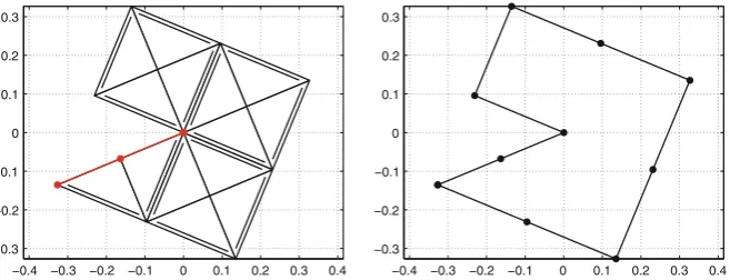
Fig. 4 Initial mesh in FE Example4.1with 14 rectangular elements (le f t) and initial mesh in BE Exam-ple4.2with 10 affine boundary segments (r ight). The reference edges for the newest vertex bisection in the FE mesh are indicated by double li nes, and the nodes on the Dirichlet boundary are indicated by
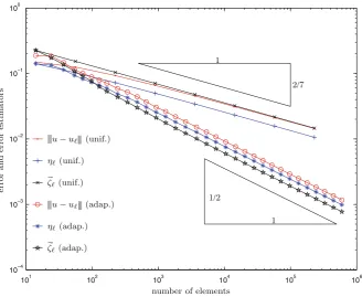
Fig. 5 Error|||u−u||| = ∇(u−u)L2()and error estimatorsηandζ=(μ2+osc2)1/2for uniform and adaptive FEM in Example4.1, where we useθ=0.25 andζfor marking in Algorithm1. Note that the adaptive strategy yields the optimal order of convergence
vergenceO(N−2/7). The optimal order of convergenceO(N−1/2)is recovered by use of the adaptive algorithm.
4.2 Boundary element method in 2D
In this experiment, we consider Symm’s integral equation
V u=(K+1/2)g (57)
which is equivalent to the Dirichlet problem
−U =0 in,
(58)
U =g on.
In this case, the exact solution of (57) is the normal derivative u=∂nU of U ∈ H1(),
Fig. 6 Error|||u−u||| ∼ u−uH−1/2()and error estimatorsηandμfor uniform and adaptive BEM in Example4.2, where we useθ =0.25 andμfor marking in Algorithm1. Note that the adaptive strategy yields the optimal order of convergence
−1 −0.5
0 0.5
1 −1 −0.5
0 0.5
1
−1 −0.8 −0.6 −0.4 −0.2 0 0.2 0.4 0.6 0.8 1
−1 −0.5
0 0.5
1 −1 −0.5
0 0.5
1
−1 −0.8 −0.6 −0.4 −0.2 0 0.2 0.4 0.6 0.8 1
Fig. 7 Initial mesh with N=96 r ectangular tr i angles (le f t) andμ-adaptively generated mesh with
N=20.806 tr i angles (r ight) in Example4.3
(K g)(x)=
C∂n(y)G(s,y)g(y)dsy for x ∈
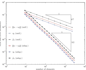
[image:24.439.58.384.368.483.2]Fig. 8 Error|||u−u||| ∼ u−uH−1/2()and error estimatorsηandμfor uniform and isotropic adaptive BEM in Example4.3, where we useθ=0.25 andμfor marking in Algorithm1
of the single-layer potential. The initial BE meshT0with N =10 affine boundary segments is shown in Fig.4.
If the normal derivative u = ∂U/∂n of U is a piecewise H1 function then the optimal order of convergence in this experiment isO(N−3/2), in terms of the num-ber N =#T of elements [20]. The numerical results are shown in Fig.6, where we again useθ=0.25 andμfor marking in the adaptive algorithm. The adaptive mesh-refinement is performed as described in Sect.3.2. Uniform mesh-refinement leads to a suboptimal order of convergenceO(N−4/7). This is cured by the adaptive algorithm in the sense that the optimal order of convergence is recovered.
For both, uniform and adaptive mesh-refinement, we observe that the error estima-torsηandμremain parallel with|||u−u|||. This strongly indicates reliability ofη and thus numerically verifies the saturation assumption (5) for this experiment.
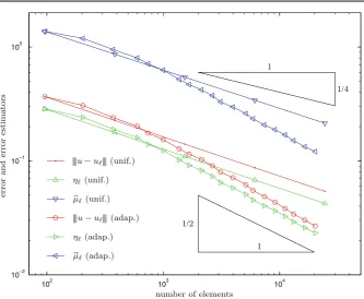
4.3 Boundary element method in 3D
Finally, we compute the discrete solution of Symm’s integral equation
withthe boundary of the Fichera cube= [−1,1]3\([0,1] × [−1,0] × [0,1]). Figure7shows the uniform initial meshT0consisting of N =96 rectangular triangles. To illustrate the performance of Algorithm1, Fig.8shows the error|||u−u|||and the estimatorsη andμ for uniform and adaptive mesh-refinements. For adaptive mesh-refinement, we use θ = 0.25 andμ in Algorithm1. Moreover, we use the bisec5-based mesh-refinement from Sect.2.2. We observe that uniform mesh-refine-ment leads to a suboptimal order of convergence of approximatelyO(N−1/4). The isotropic adaptive strategy leads to an improved order of approximatelyO(N−1/2). This, as expected, is not optimal since isotropic mesh-refinement does not resolve the generic edge-singularities efficiently [14]. For this fact, the reader is also refered to some heuristics from [8]. As in the previous example, both adaptive and uniform mesh-refinement suggest reliability ofη. This gives empirical evidence for the sat-uration assumption (5), which is required in Theorem7to guarantee convergence of the adaptive scheme.
Acknowledgements Parts of the results have been achieved during a research stay of C.O. and D.P. at the Hausdorff Institute for Mathematics in Bonn, which is thankfully acknowledged. S.F. acknowledges a grant of the graduate school Differential Equations – Models in Science and Engineering, funded by the Aus-trian Science Fund (FWF) under grant W800-N05. D.P. is partially supported through the research project
Adaptive Boundary Element Method, funded by the Austrian Science Fund (FWF) under grant P21732.
Open Access This article is distributed under the terms of the Creative Commons Attribution Noncom-mercial License which permits any noncomNoncom-mercial use, distribution, and reproduction in any medium, provided the original author(s) and source are credited.
References
1. Ainsworth, M., Oden, J.T.: A posteriori error estimation in finite element analysis. Wiley-Interscience [John Wiley & Sons], New-York (2000)
2. Bänsch, E.: Local mesh refinement in 2 and 3 dimensions. IMPACT Comput. Sci. Eng. 3, 181– 191 (1991)
3. Bank, R.: Hierarchical bases and the finite element method. Acta Numerica 5, 1–45 (1996) 4. Bank, R., Smith, R.: A posteriori error-estimates based on hierarchical bases. SIAM J. Numer.
Anal. 30, 921–935 (1993)
5. Bank, R., Weiser, A.: Some a posteriori error estimators for elliptic partial differential equations. Math. Comp. 44, 283–301 (1985)
6. Bornemann, F., Erdmann, B., Kornhuber, R.: A-posteriori error-estimates for elliptic problems in 2 and 3 space dimensions. SIAM J. Numer. Anal. 33, 1188–1204 (1996)
7. Carstensen, C., Faermann, B.: Mathematical foundation of a posteriori error estimates and adap-tive mesh-refining algorithms for boundary integral equations of the first kind. Eng. Anal. Bound. Elem. 25, 497–509 (2001)
8. Carstensen, C., Maischak, M., Praetorius, D., Stephan, E.P.: Residual-based a posteriori error estimate for hypersingular equation on surfaces. Numer. Math. 97(3), 397–425 (2004)
9. Carstensen, C., Praetorius, D.: Averaging techniques for the effective numerical solution of Symm’s integral equation of the first kind. SIAM J. Sci. Comput. 27, 1226–1260 (2006)
10. Cascon, J., Kreuzer, C., Nochetto, R., Siebert, K.: Quasi-optimal convergence rate for an adaptive finite element method. SIAM J. Numer. Anal. 46, 2524–2550 (2008)
11. Deuflhard, P., Leinen, P., Yserentant, H.: Concepts of an adaptive hierarchical finite element code. IMPACT Comput. in. Sci. and Eng. 1, 3–35 (1989)
13. Dörfler, W., Nochetto, R.: Small data oscillation implies the saturation assumption. Numer. Math. 91, 1–12 (2002)
14. Ferraz-Leite, S., Praetorius, D.: Simple a posteriori error estimators for the h-version of the boundary element method. Computing 83, 135–162 (2008)
15. Graham, I., Hackbusch, W., Sauter, S.: Finite elements on degenerate meshes: inverse-type inequalities and applications. IMA J. Numer. Anal. 25, 379–407 (2005)
16. Hairer, E., Nørsett, S., Wanner, G.: Solving ordinary differential equations I. Nonstiff problems. Springer, New York (1987)
17. Kossaczky, I.: A recursive approach to local mesh refinement in two and three dimensions. J. Comput. Appl. Math. 55, 275–288 (1995)
18. McLean, W.: Strongly elliptic systems and boundary integral equations. Cambridge University Press, Cambridge (2000)
19. Morin, P., Nochetto, R., Siebert, K.: Data oscillation and convergence of adaptive FEM. SIAM J. Numer. Anal. 38, 466–488 (2000)
20. Sauter, S., Schwab, C.: Randelementmethoden: Analyse, Numerik und Implementierung schneller Algorithmen. Teubner Verlag, Wiesbaden (2004)
21. Sewell, E.: Automatic generation of triangulations for piecewise polynomial approximations. Ph.D. thesis, Purdue University, West Lafayette (1972)
22. Verfürth, R.: A posteriori error estimation and adaptive mesh refinement techniques. J. Comput. Appl. Math. 50, 67–83 (1994)