http://wrap.warwick.ac.uk/
Original citation:
Ortner, C. and Süli, E. (2008). Analysis of a quasicontinuum method in one dimension.
ESAIM: Mathematical Modelling and Numerical Analysis, 42(1), pp. 57-91.
Permanent WRAP url:
http://wrap.warwick.ac.uk/43814
Copyright and reuse:
The Warwick Research Archive Portal (WRAP) makes this work of researchers of the
University of Warwick available open access under the following conditions. Copyright ©
and all moral rights to the version of the paper presented here belong to the individual
author(s) and/or other copyright owners. To the extent reasonable and practicable the
material made available in WRAP has been checked for eligibility before being made
available.
Copies of full items can be used for personal research or study, educational, or
not-for-profit purposes without prior permission or charge. Provided that the authors, title and
full bibliographic details are credited, a hyperlink and/or URL is given for the original
metadata page and the content is not changed in any way.
Publisher’s statement:
© EDP Sciences
http://dx.doi.org/10.1051/m2an:2007057
A note on versions:
The version presented in WRAP is the published version or, version of record, and may
be cited as it appears here.
Vol. 42, N 1, 2008, pp. 57–91 www.esaim-m2an.org
DOI: 10.1051/m2an:2007057
ANALYSIS OF A QUASICONTINUUM METHOD IN ONE DIMENSION
∗Christoph Ortner
1and Endre S¨
uli
1Abstract. The quasicontinuum method is a coarse-graining technique for reducing the complexity of atomistic simulations in a static and quasistatic setting. In this paper we aim to give a detaileda priori
anda posteriorierror analysis for a quasicontinuum method in one dimension. We consider atomistic models with Lennard–Jones type long-range interactions and a QC formulation which incorporates several important aspects of practical QC methods. First, we prove the existence, the local uniqueness and the stability with respect to a discrete W1,∞-norm of elastic and fractured atomistic solutions. We use a fixed point argument to prove the existence of a quasicontinuum approximation which satisfies a quasi-optimala priorierror bound. We then reverse the role of exact and approximate solution and prove that, if a computed quasicontinuum solution is stable in a sense that we make precise and has a sufficiently small residual, there exists a ‘nearby’ exact solution which it approximates, and we give an
a posteriori error bound. We stress that, despite the fact that we use linearization techniques in the analysis, our results apply to genuinely nonlinear situations.
Mathematics Subject Classification. 70C20, 70-08, 65N15.
Received October 11, 2006. Revised April 17, 2007.
1.
Introduction
For the numerical simulation of microscopic material behaviour such as crack-tip studies, nano-indentation, dislocation motion, etc., atomistic models are often employed. However, even on the lattice scale, they are prohibitively expensive and, in fact, inefficient. Even in the presence of defects, the bulk of the material will deform elastically and smoothly. It is therefore advantageous to couple the atomistic simulation of a defect with a continuum or continuum-like model away from it. One of the simplest and most popular examples is the quasicontinuum (QC) method originally developed by Ortizet al.[18] and subsequently improved by many other authors; see [16] for a recent survey article. The basic idea of the QC method is to triangulate an atomistic body as in a finite element method and to allow only piecewise affine deformations in the computation, thus considerably reducing the number of degrees of freedom. By taking every atom near a defect to be a node of the triangulation, one obtains a continuum description of the elastic deformation while retaining a full atomistic description of the defect. We give a detailed description of a version of the QC method analyzed in this paper in Section 2.2.
Keywords and phrases. Atomistic material models, quasicontinuum method, error analysis, stability.
∗ The authors acknowledge the financial support received from the European research project HPRN-CT-2002-00284: New
Materials, Adaptive Systems and their Nonlinearities. Modelling, Control and Numerical Simulation, and the kind hospitality of Carlo Lovadina and Matteo Negri (University of Pavia).
1 Oxford University Computing Laboratory, Wolfson Building, Parks Road, Oxford OX1 3QD, UK.
christoph.ortner@comlab.ox.ac.uk; endre.suli@comlab.ox.ac.uk
c
EDP Sciences, SMAI 2008
Interaction potential
z
J
(
z
)
zm zt
[image:3.595.115.443.123.265.2]0.0 zc
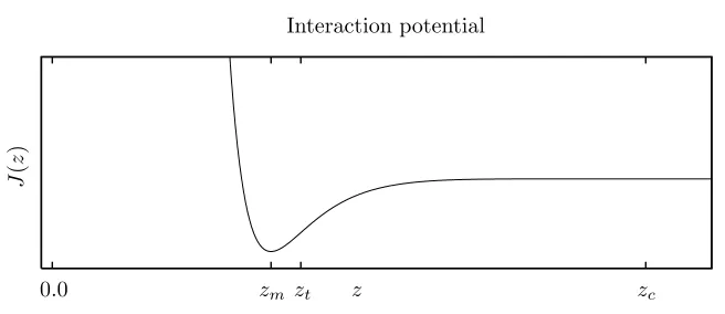
Figure 1. The shape of the atomistic interaction potentials with cut-off radiuszc.
Despite its growing popularity in the engineering community, the mathematical and numerical analysis of the QC method is still in its infancy. The first noteworthy analytical effort was by Lin [14] who considers the QC approximation of the reference state (without boundary displacements or applied forces) of a one-dimensional Lennard–Jones model. He proves that the global energy minimum of the full atomistic model as well as that of the reduced QC model lie in a region where the interaction potential is uniformly convex and uses these facts to derive an a priorierror estimate.
E and Ming [9, 10] analyze the local QC method in the context of the heterogeneous multiscale method [8], which requires the assumption that a nearby smooth, elastic continuum solution is available. The error is estimated in terms of the atomic spacing in relation to the domain size as well as the mesh size.
In [15], Lin gives a priori error estimates for a modified version of the local QC method for purely elastic deformation in two dimensions without using such an assumption, but making instead a strong hypothesis (Assumptions 1 and 2 in [15]) on the exact solution of the atomistic model as well as on its QC approximation. Essentially, he assumed generally what he was able to prove in one dimension, namely that both the exact and the QC solution lie in a region where the atomistic energy is convex. For lattice domains resembling smooth or convex sets this assumption seems intuitively reasonable but would still be difficult to verify rigorously. For lattice domains with ‘sharp’, ‘re-entrant’ boundary sections or defects we should not expect this assumption to hold, at least not in the form used in [15]. Some indication is also given as to how the analysis might be extended to the case of localized defects.
Dobson and Luskin [6] give the first analysis of some important aspects of most practical QC methods, partic-ularly the force-based approximation and the interface between regions where different types of approximation are used (see also Sect. 2.2) which requires a so-called ghost-force correction.
Finally, we mention the work of Blanc et al. [1] where a multiscale method similar to the QC method is analyzed. Only nearest-neighbour interactions in one dimension are considered which makes it possible to compute the exact solutions analytically. Nevertheless, it must be emphasized that this is the only analytical work, so far, to consider defects.
To the best of our knowledge, thea posteriorierror analysis of the QC method has not so far been considered in the literature.
The present work is an effort to unify and generalize previous results and to provide a fairly complete approximation theory for the QC method in one dimension. We demonstrate how to derive optimal a priori
error estimates for stable solutions, i.e., strict local minimizers of the atomistic energy. In order to keep the presentation simple, we consider only long-range (in the sense that any two atoms interact and that J(r) is non-zero for all r; cf. (1)) pair-interaction energies with interaction potentials of Lennard–Jones type, but we believe that this is not a true restriction. A detailed description of our model problem is given in Section 2.1.
Under sufficiently strong assumptions on the exact and the QC solution (in essence, one would have to assume a fairly stronga prioribound on a discrete W1,∞-norm of the error) it is always possible to prove quasi-optimal approximation error bounds, for example, with respect to H1-type norms. Thus, our aim in this paper is to identify situations in which such assumptions are justified. Our primary concern is to be able to answer the following two central questions:
(i) Under what conditions does a QC solution exist which approximates a given exact solution of the atomistic model?
(ii) Given a computed QC solution, does an exact solution of the atomistic model approximated by the QC solution exist?
The answer to both questions is in general negative. However, at least in the one-dimensional setting of this paper we are able to give precise conditions under which they can be answered positively. Thea priorianalysis, related to question (i), is contained in Sections 3 and 4,cf.in particular Theorems 3.2 and 4.2. The preliminary results, Theorems 3.1 and 4.1, and the discussion in Appendix B show that the conditions can be satisfied in practise and are reasonably sharp. The a posteriori existence condition, raised in question (ii), is analysed in Section 5, in Theorems 5.1–5.3. We conclude in Section 6 with a numerical example which clearly demonstrates that our analysis is both non-trivial and sufficiently sharp that it can be applied to a wide range of genuinely nonlinear situations.
We would like to emphasize the last point further. Our use of the Inverse Function Theorem and similar techniques may give the impression that our analysis is only valid in the linearly elastic regime. This is, however, not the case. Since we linearize around an arbitrary solution, our results apply to genuinely nonlinear situations. Indeed, in the numerical example that we consider, the benchmark problem ranges from the linearly elastic regime to finite elasticity and fracture.
Both question (i) and (ii) are of course fundamental questions which should be raised for any nonlinear problem. We refer to the work of Brezziet al.[5] for ana priorianalysis of this flavour and to the review article by Plum [22] for a similara posteriorianalysis (though with slightly different techniques and different aims).
We conclude the introduction by fixing some notation for discrete function spaces and nonlinear functionals.
1.1.
Discrete function spaces
It will be notationally convenient to define discrete versions of the usual Sobolev norms. First, for u = (ui)Ni=0 ∈RN+1, we introduce the discrete derivatives
u
i=
ui−ui−1
ε , i= 1, . . . , N, and ui =
ui+1−2ui+ui−1
ε2 , i= 1, . . . , N−1,
we define the (semi-)norms
up
ε((i1,i2)) =
i
2
i=i1
ε|ui|p
1/p
,
|u|w1,p
ε ((i1,i2)) =
i
2
i=i1+1
ε|ui|p
1/p
, and
|u|w2,p
ε ((i1,i2)) =
i
2−1
i=i1+1
ε|u
i|p
1/p
.
Forp=∞, we define the corresponding versions,
u∞
ε ((i1,i2)) = i=maxi 1,...,i2|
ui|,
|u|w1,∞
ε ((i1,i2)) = i=i1max+1,...,i2|u
i|, and
|u|w2,∞
ε ((i1,i2)) = i=i1+1max,...,i2−1|u
i|.
Sums or maxima taken over empty sets are understood to be zero. If the label ((i1, i2)) is omitted we mean
i1= 0, i2=N. For reasons that will become apparent below, we will only require the casesp= 1,2,∞of these (semi-)norms in our analysis. B(y, R) is understood to be the closed ball, centrey, radiusR, with respect to the w1ε,∞-semi-norm.
Foru, v∈RN+1, we define the bilinear form
u, vε= N
i=0
εuivi.
1.2.
Functionals
We fix the notation for derivatives of functionals. Letφ: RN+1 →Rbe differentiable at a pointu∈RN+1. We understand the derivative ofφat uas a linear functionalφ(u) =φ(u;·) :RN+1→Rdefined by
φ(u+v) =φ(u) +φ(u;v) +o(|v|), asv→0,
where |v| denotes the Euclidean norm of v. Similarly, if φ is twice differentiable at u ∈ RN+1, the second derivative ofφatuis a symmetric bilinear formφ(u) =φ(u;·,·) :RN+1×RN+1→Rdefined by
φ(u+v) =φ(u) +φ(u;v) +φ(u;v, v) +o(|v|2), as v→0.
When φ is interpreted as a linear functional we may also write φ(u;v) = φ(u)v. Similarly, we shall write
2.
Model problem and QC approximation
2.1.
The atomistic model problem
Fix N ∈N. Each vector y = (yi)Ni=0 ∈RN+1 represents a state of an atomistic body, consisting of N+ 1 atoms. To each suchdeformation we associate a pair-potential energy
E(y) = N
i=1 i−1
j=0
J(yi−yj).
Upon defining thelattice parameterε= 1/N, and writingyi instead ofεyi we can rescale the energy to
E(y) = N
i=1 i−1
j=0
εJε−1(yi−yj), (1)
without changing the problem. Such a scaling highlights the practically relevant case where ε is small in comparison to the length-scale of the problem.
Typical examples of atomistic interaction potentials are the Lennard–Jones potential [12],
J(z) =Az−12−Bz−6, (2)
and the Morse potential [17],
J(z) = exp−2α(z−1)−2 exp−α(z−1); (3)
see also Figure 1 (the cut-off radius zc will become important in the QC approximation and should be ig-nored for the time being). More generally, we assume that there exist z0 ∈ [−∞,+∞), zm, zt > 0 such that z0< zt/2< zm< zt,
J ∈C3(z0,∞), J(zm) = 0, J(zt) = 0,
J(z)→+∞asz→z0+, J(z) = +∞ ∀z≤z0, (4)
J(z)≥0 ∀z∈(0, zt] and J(z)≤0 ∀z∈[z
t,∞).
The only condition which is not entirely natural is the assumptionzt/2< zm, which considerably simplifies the analysis and is not a true restriction – any realistic interaction potential should satisfy this. For example, it is satisfied for the Lennard–Jones potential (2) for all positive parameters A, B, and for the Morse potential (3) wheneverα >ln 2.
Before we define what we mean by an atomistic solution, we need to mention that atomistic deformations are typically only local minimizers rather than global minimizers (cf. for example [19, 23]). This can be best seen by considering an atomistic body which is clamped at the left-hand end with a small deformation applied to the right-hand end. In that case, the physically observed Cauchy–Born state, the (approximately) affine deformation, is not the energy minimum. Note, however, that theelasticstate is the correct solution only if we havestarted from an unfractured reference state.
We consider a ‘Dirichlet’ problem where the atomistic deformation is prescribed at the endpoints. It would also be possible, and in fact easier, to consider a problem with a Dirichlet condition at one end and a Neumann condition at the other end of the interval. Given a prescribed boundary deformationyDN >0, we define the set of admissible deformations and the set of test functions respectively as
A =y∈RN+1:y0= 0, yN =yND
Each f ∈ RN+1 represents a linear body force. The atomistic problem is to find a critical point of the functionalE(y)− f, yεinA. From the assumptions we have made on the interaction potential it follows that
E is differentiable at every point which has finite energy. Thus, a critical pointy ofE(y)− f, yεin A with finite energy must satisfy
E(y;v) =f, vε ∀v∈A
0. (6)
Ify satisfies (6), we say thatE(y) =f inA.
By a solutionwe mean a critical point ofE(y)− f, yε,i.e., an atomistic deformation satisfying (6). By a
stable solutionwe mean a strict local minimizer ofE(y)− f, yε.
Elastic deformations are those whose gradient is sufficiently close to zm, in a region where the potential J is convex. Such solutions exist wheneverf is sufficiently small. This is measured with respect to thenegative norm
f∗= maxv∈A
0
|v|
w1ε,1=1
f, vε.
Since we can interpretf as a linear functional, we can extend the definition of the negative norm to linear maps
:A0→Rby
∗= max
v∈A0
|v|
w1ε,1=1
|(v)|.
For future reference, we define the quantities
ρ1(z) =
∞
r=2
(r−1)|J(rz)|, and (7)
ρ2(z1, z2) =
∞
r=1
r2 min z1≤z≤z2
J(rz), (8)
which are important in the analysis of existence and stability of elastic deformations. Forz∈(0,∞) fixed, the quantity ρ1(z) is an estimate for the residual of the affine deformationyi =zi/N which we use to derive the existence of a reference state. We shall assume throughout thatρ1is continuous in a neighbourhood ofzmwhich, for the Lennard–Jones and the Morse potentials, follows from elementary calculus. The number ρ2(z1, z2) is used to estimate the inf-sup constant ofEin the set{z1≤yi≤z2}. For the analysis of the QC approximation, we will also use
ρ3(z1, z2) =
∞
r=1
r2 max z1≤z≤z2|
J(rz)|, (9)
which is a Lipschitz constant of E in the set{z1≤yi≤z2}.
2.2.
Quasicontinuum approximation
A QC meshT is defined by choosing indices 0 =t0 < t1<· · ·< tK =N and setting T ={t0, . . . , tK}. For eachk= 1, . . . , K, we set hk =ε(tk−tk−1), the physical length of thekth element. The set of piecewise affine deformations is given by
S1(T) =V ∈RN+1:V
i= t tk−i
k−tk−1Vtk−1+
i−tk−1
tk−tk−1Vtk if tk−1≤i≤tk .
We define the set of admissible QC deformations and QC test functions respectively as
For convenience, we sometimes use the notation Vk = Vtk for the nodal values of an S1(T) function, and Vk =Vtkfor its derivatives. For our analysis it is also necessary to define the interpolant Π : RN+1→S1(T) by Πu= (Πui)Ni=0 and
Πutk=utk, k= 0, . . . , K.
Note that ify∈A then Πy∈A(T).
The Galerkin approximation of (6) in A(T) is tofind critical points of E(Y)− Y, fε in A(T). Any such critical pointY ∈A(T) must satisfy
E(Y;V) =f, Vε ∀V ∈A
0(T). (10)
However, in view of the long-range atomistic interaction, which, for the purpose of evaluating the energy and its derivatives still requires the computation of very large sums, it is helpful to make some further approximations to the energy functional. First, it is common to replace J by a cut-off potential ˜J, which vanishes outside a certain cut-off radiuszc (cf. Fig. 1). In this case, if the deformation gradient is bounded away from zero, then the number of atoms over which one needs to sum is bounded by a small integer. This purely one-dimensional effect means that it is unnecessary to make any further (summation-rule type) approximations to the atomistic energy; thus we define
˜
E(Y) = N
i=1 i−1
j=0
εJ˜ε−1(Yi−Yj).
For the stability analysis of the QC approximation we will need the quantity
˜
ρ2(z1, z2) =
∞
r=1
r2 min z1≤z≤z2
˜
J(rz).
To approximate the body force potential, we can use a so-called summation rule, i.e., a discrete version of a quadrature rule. In order to recover the full atomistic problem in the limit, it is reasonable to employ a trapezium rule. Thus, we define the discrete bilinear form
f, vT = N
i=0
εΠ(fv)i.
The QC approximation to (6) which we analyze in this paper is tofindY ∈A(T)satisfying
˜
E(Y;V) =f, V
T ∀V ∈A0(T). (11)
2.3.
Stable equilibria
In this work, we only analyze ‘stable equilibria’ of the atomistic energy (1) and the corresponding QC approximation. In principle, we would like to include all critical points y in our definition for whichE(y;·,·) is positive definite. However, we shall be slightly more restrictive. Motivated by Proposition 2.1 below, we shall only analyze purely elastic deformations and deformations which have a singlefracture,i.e., a deformation gradientyξ ztfor exactly oneξ∈ {1, . . . , N}.
In the following result we state the unsurprising fact that critical points with more than one fracture cannot be uniform local minima ofE. Fory∈RN+1, we useλ(y) to denote the smallest w1ε,2-eigenvalue ofE(y),i.e.,
λ(y) = min
u∈A0
|u|
w1ε,2=1
E(y;u, u).
Proposition 2.1. If y∈RN+1 with yp ≥zt andyq ≥zt, where 1≤p < q≤N, then λ(y)≤0. If yp or yq is
strictly greater than but sufficiently close tozt, or ifJ is strictly increasing in(zt,+∞), then λ(y)<0.
The proof of Proposition 2.1 will be given in Section 3.1. The result allows us to divide the stable critical points into two groups: elasticdeformation (analyzed in Sect. 3) andfractureddeformation (analyzed in Sect. 4).
3.
Elastic deformation
Theorem 3.1. Let J satisfy the assumptions of Section 2.1 and, in addition, assume that there exists an R∈(0,min(zm−zt/2, zt−zm))such that2ρ1(zm)< R ρ2(zm−R, zm+R); then, the following hold:
(a) Coercivity: There existz1, z2∈R, independent of ε, such thatz1< zm< z2< ztand
min y∈Ze
min
u∈A0
|u|
w1ε,∞=1
max
v∈A0
|v|
w1ε,1=1
E(y;u, v)≥1
2ρ2(z1, z2) =:c0>0, (12)
whereZe={y∈RN+1:z1≤yi≤z2, fori= 1, . . . , N}.
(b) Existence: Let z1, z2 be as in (a). There existδ1, δ2>0, independent of ε, such that for everyyDN ∈R with |yDN −zm| < δ1 (see (5) for the definition of yND) and for every f ∈RN+1 with f∗ ≤δ2, there exists a solution yf of (6)inZe.
(c) Stability: Letz1, z2 be as in(a). Letyf, yg be solutions to (6)in Ze∩A, corresponding respectively to
the right-hand sides f, g∈RN+1; then
|yf−yg|w1,∞
ε ≤c
−1
0 f −g∗.
Theorem 3.1 is of theoretical relevance in that it gives a relatively sharp condition under which elastic solutions to (6) exist and are stable. It furthermore directly relates the shape of the interaction potential to the coercivity of the energy. In practise, we would numerically determine a region where E is coercive and then prove that it contains a reference state, i.e., a deformationy∗ such thatE(y∗) = 0, using the condition
ρ1(zm)<min(zm−z1, z2−zm)ρ2(z1, z2). We demonstrate this in Appendix B.
For the formulation and proof of the a priori error bound, there are several options. One could simply formulate a QC version of the existence theorem and prove that the elastic QC solution satisfies an error estimate. However, it seems more illuminating to make fewer assumptions on the structure of the problem, and impose stronger assumptions on a particular solution instead.
For any givenf ∈RN+1and a solutiony∈A of (6), we identify three error sources: the interpolation error,
E1=|y−Πy|w1,∞
the perturbation of the linear form,
E2= max
V∈A0(T)
|V|
w1ε,1=1
f, VT − f, Vε, (14)
and the perturbation of the energy,
E3=Y max
∈A(T)∩Ze
max
V∈A0(T)
|V|
w1ε,1=1
E(Y;V)−E˜(Y;V). (15)
Theorem 3.2.
(a) Let Ze be defined as in Theorem3.1; then,
min
Y∈S1(T)∩Ze U∈minA0(T)
|U|
w1ε,∞=1
max
V∈A0(T)
|V|
w1ε,1=1
E(Y;U, V) ≥ 1
2ρ2(z1, z2) =c0, and (16)
max
Y∈S1(T)∩Ze U∈maxA0(T)
|U|
w1ε,∞=1
max
V∈A0(T)
|V|
w1ε,1=1
E(Y;U, V) ≤ ρ
3(z1, z2) =:c1. (17)
(b) Let y ∈ Ze∩A be a solution of (6) and define R = mini=1,...,Nmin(z2−yi, yi −z1). Assume, furthermore, that the QC meshT and the cut-off radius are such that
c1E1+E2+E3≤c0R. (18)
Then, there exists a solutionY ∈A(T)∩Ze to (11)which satisfies
|y−Y|w1,∞
ε ≤c
−1
0
(c0+c1)E1+E2+E3.
If ρ˜2(z1, z2)>0, then the QC solution is unique in A(T)∩Ze. (c) The error quantitiesE1,E2 andE3 can be bounded as follows:
E1 ≤ 12kmax
=1,...,Khk|y|wε2,∞((tk−1,tk)), (19)
E2 ≤ max k=1,...,Kh
2 kmax
|f|w2,∞
ε ((tk−1,tk)),2|f|wε1,∞((tk−1+1,tk))+ 2|f|wε1,∞((tk−1,tk−1))
, and (20)
E3 ≤ ∞
r=1
r max z1≤z≤z2
J˜(rz)−J(rz). (21)
3.1.
Coercivity of the atomistic problem
For this fairly straightforward but tedious analysis it is convenient to rewrite the energy and its derivatives in the following form. First, we rewriteE as
E(y) = N
i=1 i
j=1
εJ i
k=j
y
k
For the moment we will only needE, however, for future reference we first computeE which can be written in the form
E(y;w) =
N i=1 i j=1 εJ i
k=j
y
k
i
n=j
w n = N i=1 i j=1 i
n=j
εw
nJ
ε−1(yi−yj
−1)
= N i=1 i n=1 εw n n j=1
Jε−1(yi−yj
−1) =
N n=1 εw n N
i=n n
j=1
Jε−1(yi−yj
−1)
= N n=1 εF
n(y)wn, (23)
where
F
n(y) = N
i=n n
j=1
Jε−1(yi−yj
−1).
Here and below we shall use the notationn∨m= min(n, m) andn∧m= max(n, m). IfEis twice differentiable at a pointy, thenE(y;v, w) is more conveniently written in the form
E(y;v, w) =
N i=1 i j=1
εJε−1(yi−yj
−1)
i
m=j
v
m
i
n=j
w n = N n=1 εw n N
i=n n
j=1 i
m=j
v
mJ
ε−1(yi−yj
−1)
= N n=1 εw n N
i=n i
m=1 n∧m
j=1
v
mJ
ε−1(y
i−yj−1)
= N n=1 N m=1 εw
nvm
N
i=m∨n n∧m
j=1
Jε−1(yi−yj
−1)
= N n=1 N m=1 εF
nmvm wn, (24)
where
F
nm(y) = N
i=m∨n n∧m
j=1
Jε−1(y
i−yj−1).
As a first application of this decomposition, we give the proof of Proposition 2.1.
Proof of Proposition 2.1. We perturb y with a displacementu∈A0 such that
u
i=
⎧ ⎨ ⎩
−ε−1/2, if i=p,
Then,|u|2
w1ε,2 = 2 and, recalling thatp < q,
E(y;u, u) = F
pp+Fqq −2Fpq
= N
i=p p
j=1
Jε−1(yi−yj
−1)+
N
i=q q
j=1
Jε−1(yi−yj
−1)−2
N
i=q p
j=1
Jε−1(yi−yj
−1)
= q−1
i=p p
j=1
Jε−1(y
i−yj−1)+ N
i=q q
j=p+1
Jε−1(y
i−yj−1).
Sinceyp, yq≥ztit follows thatJ(ε−1(yi−yj−1))≤0 for alliandj appearing in the last two sums. If either
y
p or yq is strictly greater than but sufficiently close to zt, or if J < 0 in (zt,+∞), then this expression is
negative. Hence the result follows.
We now continue with the proof of coercivity of the atomistic problem. Our aim in this section is to identify a set of deformations,
Ze={y∈A :z1≤yi≤z2},
withz1< zm< z2< ztfor whichE(y;·,·) satisfies the inf-sup condition
min y∈Ze
min
u∈A0
|u|
w1ε,∞=1
max
v∈A0
|v|
w1ε,1=1
E(y;u, v)≥c 0>0.
For convenience, we have assumed in Section 2.1 thatzm> zt/2, and hence we may assume here thatz1≥zt/2 as well. This implies that
J(z)>0, forz
1≤z≤z2, and
J(z)≤0, forz≥2z
1, (25)
and consequentlyFnm ≤0 whenevern=m.
The proof of the inf-sup condition is based on an argument related to row-diagonally-dominant matrices. Fix u∈A0 and choosep, q ∈ {1, . . . , N} such that up is maximal and uq is minimal. Since u∈A0 we have
N
i=1ui= 0 and henceup≥0 anduq ≤0. We define the test functionvby
v i= ⎧ ⎨ ⎩ 1
2ε−1, if i=p, −1
2ε−1, if i=q, and 0, otherwise.
It is clear from this definition that v ∈ A0 and |v|w1,1
ε = 1. Let P = {i : u
i > 0} and Q = {i : ui < 0}. Using (24), we have
E(y;u, v) = N
n=1 N
m=1
εF
nm(y)unvm
= 1 2ε N n=1 εF
np(y)un− 1 2ε
N
n=1
εF
nq(y)un
= 1
2F
pp(y)up+1 2
n=p
F
npun−1 2F
qq(y)uq−1 2
n=q
F
Using (25), we see that forn=mwe haveFnm (y)≤0. Hence, we obtain
2E(y;u, v) ≥ Fpp(y)up+
m∈P\{p} F
pm(y)um−Fqq(y)uq−
m∈Q\{q} F
qm(y)um
≥ u
p
F
pp(y) +
m∈P\{p} F
pm(y)
+ (−u
q)
F
qq(y) +
m∈Q\{q} F
qm(y)
≥ |u|w1,∞
ε
N
m=1
F
nm(y), (26)
where n ∈ {p, q}. Thus, to prove the coercivity estimate (12), we need to show that the matrix (Fnm )Nn,m=1 is strictly row diagonally dominant; more precisely, we need to obtain a lower bound on the sum in the last expression. To do so, we split the sum as follows:
N
m=1
F
nm(y) = n−1
m=1 N
i=n m
j=1
Jε−1(yi−yj
−1)+
N
m=n+1 n
j=1 N
i=m
Jε−1(yi−yj
−1)+
n
j=1 N
i=n
Jε−1(yi−yj
−1).
For all pairs (i, j) withi≥j we bound
J(ε−1(yi−yj
−1))≥ min
z1≤z≤z2
J(i−j+ 1)z=:J(i−j+ 1),
which we use to estimate
N
m=1
F
nm(y)≥ n−1
m=1 N
i=n m
j=1
J(i−j+ 1) + N
m=n+1 n
j=1 N
i=m
J(i−j+ 1) + n
j=1 N
i=n
J(i−j+ 1). (27)
In the first triple-sum, we exchange the order of summation three times to obtain
n−1
m=1 N
i=n m
j=1
J(i−j+ 1) = N
i=n n−1
j=1 n−1
m=j
J(i−j+ 1)
= n−1
j=1 N
i=n
(n−j)J(i−j+ 1)
≥ n−1
j=1 (n−j)
∞
r=n−j+1
J(r),
where we used the fact thatJ(r)≤0 forr≥2. We change the order of summation again to obtain
n−1
j=1 (n−j)
∞
r=n−j+1
J(r) =∞
r=2
J(r) n−1
j=n−r+1
(n−j) =1 2
∞
r=2
r(r−1)J(r),
where we used nj=−n1−r+1(n−j) =r(r−1)/2. Similarly, for the second triple-sum in (27), we obtain
N
m=n+1 n
j=1 N
i=m
J(i−j+ 1)≥ 1
2
∞
r=2
For the third term in (27), we have
n
j=1 N
i=n
J(i−j+ 1)≥
n
j=1 ∞
r=n−j+1
J(r) =∞
r=1 n
j=n−r+1
J(r) =∞
r=1
rJ(r).
On combining this with the previously obtained bounds, and recalling the definition (8), we finally arrive at
N
m=1
Fnm (y)≥
∞
r=1
r2J(r) =ρ2(z1, z2). (28)
Therefore, returning to (26), we obtain
max
v∈A0
|v|
w1ε,1=1
E(y;u, v)≥c
0|u|w1,∞
ε , (29)
where c0= 12ρ2(z1, z2). We refer to Appendix B for specific values of z1, z2 andc0 for the Lennard–Jones and the Morse potential.
Corollary 3.3. If y∈Ze thenE(y) is positive definite in
A
0={u∈RN+1:u0= 0}.
Proof. From (28) we deduce that the matrix (Fnm )Nn,m=1 is strictly row diagonally dominant. Using the repre-sentation (24), and noting that eachu∈A0 has a unique representation in terms ofu andvice versa, we can
immediately deduce thatE(y) is positive definite inA0.
3.2.
Proof of Theorem 3.1
The proof of Theorem 3.1 as well as its extension to fracture solutions in Section 4 rely on the following local existence result which is, in essence, a continuation principle for the Inverse Function Theorem.
Lemma 3.4. Let · be a norm in A0,R >0 andy˜∈A, and define Z ={y∈A :y−y˜ ≤R}. Suppose, further, that:
(i) Φ :RN+1→(−∞,+∞]is three times continuously differentiable in Z;
(ii) Φ(˜y) = ˜f inA,i.e.,Φ(˜y;v) =f, v˜ ε ∀v∈A0;
(iii) there existsc0>0 such that
c0≤min y∈Z umin∈A0
u=1
max
v∈A0
|v|
w1ε,1=1
Φ(y;u, v); and (30)
(iv) Φ(y)is positive definite for every y∈Z.
Then, for each f ∈RN+1 satisfying f −f˜∗≤c0R, there exists a uniquey ∈Z such thatΦ(y) =f in A. Furthermore, the solutiony satisfies
y−y˜ ≤c0−1f−f˜∗. (31)
Proof. As mentioned above, this result is a standard continuation principle for the Inverse Function Theorem and we therefore omit a complete proof here. We refer to the Zeidler’s monograph [25] for an extensive discussion. Let us simply note that (30) implies that Φ(y) is an isomorphism for eachy ∈Z and thus, in each point
y∈Z the Inverse Function Theorem can be applied. This fact can be used to successively solve forytgiven by Φ(yt) = (1−t) ˜f+tf. Given the conditionf−f˜∗≤c0R, it follows that this process can be continued up to
Lemma 3.4 gives a clear path to the proof of Theorem 3.1. We have already established the necessary conditions for coercivity in the previous section.
To show the existence of a reference state, we define the deformation yiD =εiyND, where yDN will be fixed later, and estimate the residual E(yD;·). It is more convenient to do this using the following alternative representation ofE(y;v):
E(y;v) =
N−1
n=1
E
n(y)vn ∀y∈A, ∀v∈A0, (32)
where
E
n(y) = n−1
i=0
Jε−1(yn−yi)− N
i=n+1
Jε−1(yi−yn), n= 1, . . . , N−1. (33)
Using the embedding inequalityv∞
ε ≤ 12|v|w1ε,1 (cf. Lem. A.3) we can estimate
|E(y;v)| ≤
N−1
n=1 |E
n(y)|v∞
ε ≤
1 2
N−1
n=1 |E
n(y)||v|w1,1
ε ,
which implies that
E(y)
∗≤ 1
2 N−1
n=1 |E
n(y)|. (34)
Setting y=yD in (33), we have
E
n(yD) =
⎧ ⎪ ⎪ ⎨ ⎪ ⎪ ⎩
2n−N−1 i=0 J
(n−i)yND
, ifn≥(N+ 1)/2, −Ni=2n+1J
(i−n)yND, ifn≤(N−1)/2,
0, otherwise,
and, taking absolute values,
|E
n(yD)| ≤
∞
r=n∧(N−n)+1
|J(ryD N)|.
Thus, we can estimate
E(yD)
∗ ≤ 12
N−1
n=1 |E
n(yD)| ≤
∞
n=1 ∞
r=n+1
|J(ryD N)|
=
∞
r=2 r−1
n=1
|J(ryD N)| =
∞
r=2
(r−1)|J(ryDN)| = ρ1(yDN).
We now apply Lemma 3.4 with Φ =E,·=|·|w1,∞
ε , ˜y=y
Dandf = 0. From the assumptions in Theorem 3.1
it follows that there existz1, z2 such that
ρ1(zm)< 12ρ2(z1, z2)×min(z2−zm, zm−z1).
Sinceρ1is assumed to be continuous it furthermore follows that there existsδ1>0 such that, for|yDN−zm| ≤δ1,
It therefore follows from Lemma 3.4 that there exists a reference statey∗∈A satisfying (6) withf = 0. From the stability estimate (31), we infer that
|y∗−yD| w1,∞
ε ≤c
−1
0 E(yD)∗≤2 ρ1(y
D N)
ρ2(z1, z2) <min(z2−y D
N, yDN −z1).
Hence, there existsR >0 such that {y ∈A :|y−y∗|w1,∞
ε ≤R} ⊂Ze. Applying Lemma 3.4 again, it follows
that, for f∗≤c0R=:δ2, there exists a unique solution to (6) inZe.
3.3.
Coercivity of the QC approximation
In order to apply a similar technique as in Section 3.2 to prove the existence of a QC solution near an exact solution, we need to show thatE is also coercive inA0(T),i.e., that there exists a constant ˜c0>0 such that
min
Y∈Ze∩A(T) U∈minA0(T)
|U|
w1ε,∞=1
max
V∈A0(T)
|V|
w1ε,1=1
E(Y;U, V)≥˜c 0.
To this end, fixU ∈A0(T) and pickp, q∈ {1, . . . , K} such thatUp is maximal andUq is minimal. Similarly as before, we also letP ={i:Ui >0}andQ={i:Ui<0}, and we define
Vk=
⎧ ⎪ ⎪ ⎨ ⎪ ⎪ ⎩ 1
2h−p1, if k=p, −1
2h−q1, if k=q, and 0, otherwise.
This gives
E(Y;U, V) = N
n=1 N
m=1
εF
nm(Y)UnVm
= 1
2hp N
n=1 tp
m=tp−1+1
εF
nm(Y)Un − 1 2hq
N
n=1 tq
m=tq−1+1
εF
nm(Y)Un
≥ U
p 2hp
tp
m=tp−1+1
ε
n∈P
F
nm(Y)−
Uq
2hq tq
m=tq−1+1
ε
n∈Q
F
nm(Y).
Using the estimate (28), we obtain
E(Y;U, V)≥ U
p 2hp
tp
m=tp−1+1
ερ2(z1, z2)− U
q 2hq
tq
m=tq−1+1
ερ2(z1, z2)≥c0|U|w1,∞
ε ,
wherec0=12ρ2(z1, z2),i.e., we have the same inf-sup constant as in the case of the full test-spaceA0. If we now replaceE by ˜E in all the above computations, we obtain instead
min Y∈A(T)∩Ze
min
U∈A0(T)
|U|
w1ε,∞=1
max
V∈A0(T)
|V|
w1ε,1=1
˜
E(Y;U, V)≥ 1
2ρ˜2(z1, z2). (36)
Corollary 3.5. Suppose that ρ˜2(z1, z2)>0. Then, for everyY ∈Ze,E˜(Y)is positive definite in
A
0(T) ={U ∈A(T) :U0= 0}.
3.4.
Proof of Theorem 3.2
Stimulated by thea priorierror analysis in [21], we begin by rewriting the QC approximation as a fixed-point problem. To this end, assume thatY ∈A(T)∩Zesatisfies (11). Lety∈A ∩Ze be an exact solution and let Πy be its interpolant. We then have, for allV ∈A0(T),
1
0
EΠy+τ(Y −Πy);Y −Πy, Vdτ =E(Y;V)−E(Πy;V) (37)
= E(Y;V)−E˜(Y;V) +f, VT − f, Vε+E(y;V)−E(Πy;V) =:Y(V).
In fact, we see thatY is a solution of (11) if, and only if, it solves (37) which we rewrite as a fixed point problem. Letϕ∈A(T)∩Ze. We define the fixed point mapL:A(T)∩Ze→A(T),Yϕ=L(ϕ) by
1
0
EΠy+τ(ϕ−Πy);Yϕ−Πy, V) dτ =ϕ(V) ∀V ∈A
0(T). (38)
Corollary 3.3 implies that there exists a uniqueYϕ satisfying (38). Furthermore, we note that the construction of the test functionV in Section 3.3 was independent of the base point and can therefore be performed uniformly for allYτ = Πy+τ(ϕ−Πy). It therefore follows immediately that
1
0 E
(Yτ;Yϕ−Πy, V) dτ≥c
0|Yϕ−Πy|w1,∞
ε ,
and we obtain
c0|Yϕ−Πy|w1,∞
ε ≤ Vmax∈A0(T)
|V|
w1ε,1=1
|ϕ(V)|=ϕ∗≤c1E1+E2+E3,
wherec1is a Lipschitz constant forE inZeandEi,i= 1,2,3, are defined at the beginning of Section 3. Thus, in order for L to mapA(T)∩Zeinto itself, it is sufficient that
c1E1+E2+E3≤c0 min
i=1,...,Nmin(Πy
i−z1, z2−Πyi).
Since Πytk =ytk fork= 0, . . . , K, it follows that
tk
i=tk−1+1
εy
i−hkΠyk= 0,
To boundE inZe, we compute
|E(θ;U, V)| =
N
n=1 N
m=1
ε|F
nm(θ)||Un|| Vm|
≤ |U|w1,∞
ε
N
m=1
ε|Vm| N
n=1 |F
nm(θ)|
≤ |U|w1,∞
ε |V|w1ε,1m=1max,...,N N
n=1 |F
nm(θ)|.
We can bound the sum in the last term by a computation identical to that in (28) except that the signs are reversed, and thus we obtain (17).
To boundE1 we simply use Theorem A.4 withp=∞. ForE2, we use Theorem A.4 withp= 1 to estimate
f, VT − f, Vε≤
N
i=1
εΠ(fV)i−fiVi≤ K
k=1
h2
k|Π(fV)|w2,1
ε ((tk−1,tk)).
Fori=tk−1+ 1, . . . , tk−1, using the fact thatVi= 0, we have
(fV)i = ε−2(fi+1Vi+1−2fiVi+fi−1Vi−1)
= fi+1−2fi+fi−1
ε2 Vi+
fi+1−fi
ε
Vi+1−Vi
ε +
fi−fi−1
ε
Vi−Vi−1
ε ·
Thus, using the discrete Friedrichs inequality (69), we obtain
f, VT − f, Vε ≤
K
k=1
h2 k
|f|w2,∞
ε ((tk−1,tk))V1ε((tk−1+1,tk−1))
+ (|f|w1,∞
ε ((tk−1+1,tk))+|f|w1ε,∞((tk−1,tk−1)))|V|wε1,1((tk−1,tk))
≤ max
k=1,...,Kh 2 kmax
|f|w2,∞
ε ((tk−1,tk)),2|f|w1ε,∞((tk−1+1,tk))
+ 2|f|w1,∞
ε ((tk−1,tk−1)) V1ε+12|V|w1ε,1
.
We apply (69) to estimateV1
ε ≤12|V|w1ε,1 and thus prove the bound (20).
Finally, defining ˜Fn analogously toFn, and using (23), the bound (21) onE3 follows from
|E(θ;V)−E˜(θ;V)| ≤N
n=1
ε|F
n(θ)−F˜n(θ)||Vn| ≤ nmax =1,...N|F
n(θ)−F˜n(θ)||V|w1,1
ε ,
and a computation that is identical to the one leading to (35).
4.
Fracture
However, even with a single fracture, it should be apparent from the analysis of Section 3.1 that we cannot expect (29) to hold when |u|w1,∞
ε =|u
ξ|sinceJ(uξ)≈0. We therefore change the norm in which we analyze the error to the norm| · |w1,∞
ε,f defined by
|u|w1,∞
ε,f = i=1max,...,N i=ξ
|ui|.
Since we have imposed a Dirichlet condition at both endpoints,|·|w1,∞
ε,f is indeed a norm onA0. We useBf(y, R)
to denote the balls, centre y and radiusR, with respect to the | · |w1,∞
ε -semi-norm. As was hinted above, we
define
Zf =y∈A :yξ ≥zf andz1≤yi≤z2 fori= 1, . . . , N, i=ξ,
where the constantszi satisfyz1< zm< z2< zt, and zf is sufficiently large (which we will make precise). In order to simplify the proofs of coercivity we assume that
J(z)≥0 forz≥zf. (39)
This typically imposes a negligible lower bound onzf. We shall also need a further measure of stability,
ρ2,f(zf, z1) =
∞
r=0
(r+ 1)2J(zf +rz1).
The definition ofρ2,f does not involvez2 because we have assumed (39). The function ˜ρ2,f corresponding to the cut-off potential ˜J is defined analogously. In order to be able to neglect the effect of long-range interactions across the crack, we assume that
∀a >0 ∀z1≥zt/2 ∃zD=zD(a, z1) : Nρ2,fN(zD−zt), z1≥ −a. (40)
This would typically involve a decay condition for J, for example, |J(z)| z−k, for some k > 3 and
z sufficiently large.
Theorem 4.1. Let J satisfy the assumptions of Section2.1as well as conditions (39)and (40). Assume also that there existsR∈(0,min(zm−zt/2, zt−zm))such that4ρ1(zm)< Rρ2(zm−R, zm+R); then, the following
hold:
(a) Coercivity: There existz1< zm< z2< ztindependent of ε, andzf =O(ε−1)such that
min y∈Zf
min
u∈A0
|u|
w1ε,f,∞=1
max
v∈A0
|v|
w1ε,1=1
E(y;u, v)≥ 1 2
ρ2(z1, z2) + 2Nρ2,f(zf, z1)=:c0>0, (41)
whereZf is defined as above.
(b) Existence: There exist δ1, δ2>0, independent ofε, such that for everyyND∈R withyDN ≥zm+δ1 and for every f ∈RN+1 with f∗≤δ2, there exists a solutionyf of (6)inZf.
(c) Stability: Let yf, yg be solutions to (6)in Zf∩A with respective right-hand sidesf andg; then
|yf−yg|w1,∞
ε,f ≤c
−1
0 f −g∗.
For the QC error bounds, letE1=|y−Πy|w1,∞
ε,f and letE2and E3be defined as in Section 3.
Theorem 4.2. Let J satisfy the conditions of Section 2.1 as well as (39)and (40), and let Zf be defined as