Improving convergence of numerical optimizers using a limited number of function evaluations

(1)

Improving convergence of

numerical optimizers using a

limited number of function

evaluations

F.J.F. Duisterwinkel

Supervisors:

Dr. D.F. De Lange

Dr. Ir. W.W. Wits

May 16, 2015

(2)

Abstract

Background: Visual control systems can be used in robot welding applica-tions to track seems. The current industry standard uses Computer Image Analysis. However this method is sensitive to bad lightning conditions and loses effectiveness when dealing with curved surfaces. An alternative concept is based on creating a virtual version of the captured image and using optimiza-tion algorithms to minimize dissimilarities between the virtual model and the actual image. This method has shown that it is less prone to lightning condi-tions and can be used to track complex surfaces. But in order to be used in a control system, the process time should be limited to reduce latency. This re-search explores a number of optimization schemes and compares their accuracy after a fixed run time. The goal of this research is to find a method to reduce the measurement error as much as possible in 50ms. Which is approximately 20 function evaluations regardless of the chosen optimization scheme, since the function evaluation is the dominant factor in the run time of an optimization step.

Results: It is shown that for this application a preprocessing step that scales the various parameters significantly increases performance. Since this is a pre-processing step it does not affect the 50msrun time constraint. Without using preprocessing a BroydenFletcherGoldfarbShanno algorithm performs best un-der the mentioned conditions. When using preprocessing the Nelun-der Mead al-gorithm performed significantly worse than its peers, while all other alal-gorithms shown acceptable errors.

Conclusion: Assuming that the initial error is small, it is possible to com-pare a captured image with a virtual reconstructed image using optimization techniques within a 50mswindow. This can be used in visual control systems, albeit this has not been tested. The program is written in _Matlab and it is conceivable that performance can be improved by translating it to an other language like C++.

(3)

Artificial analysis method

The goal of this study is to investigate the use of different computational opti-mization algorithms for their performance in an artificial vision application.

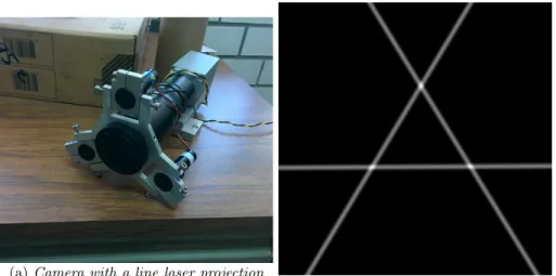
This report is an in depth analysis of a single aspect of the artificial vision application developed by Vctor Hugo Jurez Matus and is described in his master theses: ”Desarrollo y integracin de un cabezal con visin artificial con un robot”. The goal of this method is to measure the relative distance between the camera and a surface. To do this the method utilizes a camera with three line lasers attached to it as is shown in figure 1.1a. These lasers create a unique pattern for each set of camera coordinates, an example is shown in figure 1.1b. Traditionally these lines can be ’read’ using image analysis algorithms, but these methods are generally only available for straight lines and they are sensitive to imperfections and lightning conditions. So an alternative method to interpret the visual data is proposed. This alternative method utilizes an optimizing al-gorithm that minimizes the difference between the captured image and a virtual projection.

The idea of the optimization strategy is that if the set-up is calibrated cor-rectly, a virtual replication of the line pattern would create a similar image as the camera if the input coordinates of the virtual image are close to the actual coordinates of the camera. To analyse a single camera frame multiple virtual images are generated and compared to the actual image. The most similar vir-tual image is the best estimation of the coordinates. But as the creating and comparing of virtual images is a relative computational expensive operation, it is essential to use an effective optimization algorithms to reduce the computation time.

A possible application for this method is to serve as a feedback loop to determine the relative location of an actuated arm in a robot welding process. This application require a reasonably short calculation time to facilitate high movement speed while reducing positioning errors during welding. The chosen time for this is 50ms as this is similar to the limit of current image capture technology.

(5)

(a)Camera with a line laser projection

attachment (b)Captured laser projection

Figure 1.1: Camera setup and laser projection

an identical match will not be found, as a conic filter is applied to the virtual image to ’smear out’ the laser. The reason for this is that the objective function only changes significantly if the lasers overlap. But as the laser lines are quite narrow this only happens if the candidate coordinates are already very close to the actual image. By smearing out the virtual image the effective search area is increased at the expense of some accuracy.

Initial analysis show that when the optimization method does not use more than 20 function evaluations, the method is considered sufficiently quick. The challenge is to reduce the error as much as possible using just 20 function evalua-tions. Since most literature in computational optimization is focused on reaching a fixed error within a reasonable time but using a variable number of function evaluation. Directly implementing existing methods in this case resulted in hun-dreds to tens of thousand function evaluations, so the sought after maximum of 20 evaluations requires additional improvements in the method.

1.1 Objective function

The objective function for this process is a function that creates a virtual pro-jection based on the input coordinates and comparing it to the input image. The input for this function consists of n = 3 coordinates and the output is a score between 0 and 1 where a low output means a high similarity, this is done because in optimization methods the objective function should be minimized.

The objective function consists of several steps that are briefly described here, a more in depth explanation can be found in

1.1.1 Create virtual image

(6)

of three straight lines, but the same method could be adapted for use in other cases.

The captured image that has to be interpreted is a raster image with certain dimensions where each pixel has a grey scale intensity. For the comparison the virtual image should be similar to easily determine the degree of similarity. The resolution of the source image and consequentially the virtual image has a large impact on the total calculation time as both the filter and the comparing of images has to be done for more pixels. The image should have a low resolu-tion while being high enough so that the important details are preserved. In this application the resolution is kept constant at 800x800 pixels to reduce the variables of the study, but the resolution should be tweaked to allow an optimal performance while maintain a reasonable robustness.

To convert the vector information each line is decomposed into a series of dots. But as each dot location does not necessarily coincides with a single pixel, all dots are divided across 4 pixels with various intensities.

1.1.2 Apply Filter

To ensure there is some overlap between the virtual and actual lines, they both get smeared out by a conic filter. This is one of the most expensive operations in the process. There are some considerations about the filter settings, as in-creasing the filter area will increase the chance to create an overlap between the images but it also increases computational time. This is because area’s outside the filter area do not add to the computations. Because each dot is rendered as a unique combination of 4 pixels, it is not possible to apply the filter to a single dot and construct the virtual image this way. This would reduce the computational time significantly.

Another consideration is that by smearing out the image the convergence rate decreases as the gradient of the objective function as the drop from 1 to 0 gets spread out over a larger interval. This reduces the convergence rate and thus the accuracy after 20 iterations.

1.1.3 Determine degree of overlap

The final step in the objective function process is to actually compare the virtual and captured images. This is done by measuring the overlap between the two images by taking the sum over the dot product of the two image matrices as is shown in equation (1.1) where Gvir and Gcap are the matrices with greyscale

values of respectively the virtual and captured images.

y= 1−X n

X

m

(Gvir.∗Gcap) (1.1)

1.2 Candidate optimizers

(7)

the derivatives of the objective functions are not known the methods have to ap-proximate these if they are not derivative free, requiring more objective function evaluations. A forward finite difference approximation is used to approximate the derivativesf0(x). This usesn+ 1 function evaluations by computing equa-tion (1.2) for every dimension.

f(x+h)−f(x)

h =f

0₍_x_{) +}_O₍_h₎ _(1.2)

Where n is the number of dimensions (3 in this case). The error O of a forward finite difference approximation is of order h, where his the difference in coordinate between the original point and thef(x+h) point. Decreasingh

will improve the accuracy of the approximation but it might also makes it more susceptible to noise effects. This is because with the same gradient, a smaller step size makes the change is output smaller while the noise effects stay similar. Below this is a short description of the algorithms and their strengths and weaknesses. The descriptions are meant as a short introduction to the methods and are in no way a comprehensive description.

1.2.1 Downhill Simplex

Also known as the Nelder-Mead or amoeba method. It is the only 0th _order method that is included in the analysis meaning it only requires function output values but no derivatives. The basic concept of this method is that it starts with a simplex, which is any shape composed out ofn+ 1 points. Out of thesen+ 1 points it determines the point that has the worst objective value. Then a set of rules is used to determine where to move this point, alternatively it shrinks the simplex if the new point does not improve the objective function. If a two dimensional objective function is represented by a surface plot, the simplex can be illustrated as an amoeba that moves downhill on this surface towards the bottom of the valley while constantly changing shape and decreasing in size as it gets closer.

The advantage of not requiring gradient information is that it decreases the number of function evaluations per iteration, as there is no need for a forward finite difference approximation. The absence of gradient information makes the optimizer more robust to noise and non-linearities, but also limits the conver-gence rate. Returning to the analogy of an amoeba moving downhill, the method is fairly fast in moving downhill towards the valley as each step only takes 1 to 3 function evaluations. However once it is close to the optimum point it has to shrink and for this alln+ 1 points have to be recalculated on top of checking if a lateral movement will improve the objective function.

1.2.2 BFGS

This method is a quasi-Newton method, an approximation of the Newton method. The Newton method uses first and second order derivatives f0(x) andf00(x) of the objective function in a Taylor expansion to find a point x∗ that satisfies

f0₍_x

∗) = 0. In higher dimension cases the first and second order derivatives are

(8)

directly. For this reason the Hessian matrix is approximated with gradient in-formation from the previous steps, making it an quasi-Newton method.

The Broyden-Fletcher-Goldfarb-Shanno algorithm is a quasi-Newton line search method as it updates an approximated Hessian matrix Bk+1 using the approximated gradient data (1.7). The general procedure is shown in equa-tions (1.3) to (1.7).

Obtain directionpk: Bkpk=− 5f(xk) (1.3)

Find aαk with line search: xk+1=xk+αkpk (1.4)

sk=αkpk (1.5)

yk=5f(xk+1)− 5f(xk) (1.6)

Bk+1=Bk+ ykytk yt

ksk

−Bksks t kBk st

kBksk

(1.7)

pk is the search direction, ak is the step length, Bk is the Hessian matrix

approximation,sk is the difference betweenxkandxk+1andyk is the difference

in gradients.

For the initial performance analysis the build-in_Matlabfunctionfminuncis used. This isMatlab’s native function to minimize unconstrained functions. This method uses the BFGS method with a quadratic and cubic line search. However, as thefminunc function requires the optimization toolbox that is not included in older versions of Matlab. So for use with older versions of Matlab or as a standalone C++ code it should be converted into elementary operations. However the performance can be quite sensitive to the parameters of the code, and it can be challenging to replicate the code out of the Matlab library.

This algorithm is widely used because it has excellent convergence properties for many non linear optimization problems. The performance is especially good if the Jacobian can be derived analytically, for this application this is not the case thus reducing it’s convergence rate.

1.2.3 Levenberg-Marquardt

This method1_{, also known as the damped least-squares method is a} combina-tion of the Gauss-Newton algorithm (a variacombina-tion of the Newton method) and a steepest descent method. Based on the improvement in the objective func-tion relative to the previous iterafunc-tion the contribufunc-tion of one of these methods is dominant. This way the Levenberg-Marquardt(LM) method combines the quick global convergence of a gradient descent with the improved local performance of a quasi newton method.

1.2.4 Barzilai-Borwein gradient

The Barzilai-Borwein gradient method is a line search method that uses gradient information and function outputs. Each iteration only needs O(n) operations and a single gradient evaluation which needsO(n+ 1) function evaluations. The method is described by equations (1.8) to (1.10).

1_{Henri P. Gavin 2013. The Levenberg-Marquardt method for nonlinear least squares}

curve-fitting problems.

(9)

xk+1=xk−

1

αk

gk (1.8)

αk =

st_k₋₁yk−1

st k−1sk−1

(1.9)

sk−1=xk−xk−1 and yk−1=gk−gk−1 (1.10) Wherexkis thekthapproximation to the optimal solution,gkis the gradient

vector off atxk and 1/αis a step size

According to Raydan(1997)2 _{the method converges quickly for quadratic} objective functions (Section /refsec:ObjectiveFunctionAn it is shown that the objective function is approximately quadratic) as it does not require line search algorithm to determine the step length. The additional benefit of the method requiring less operations and stored variables as similar methods. This last argument is not relevant as the current application only has three dimensions but it might become more relevant in other situations. The code that is used was written by Mark Schmidt3

1.2.5 Hessian Free Newton

This algorithm is a L-BFGS written by Mark Schmidt4_{. This is essentially a} BFGS algorithm and uses the same principles described in (1.3) to (1.7) that is modified to reduce memory requirements for large problems that have hundreds to thousands variables. Although this is not necessary in this application, this method will work on older versions ofMatlabthat do not have the optimization toolbox that is required for thefminunc function mentioned in section 1.2.2.

2_{M. Raydan 1997. The Barzilai and Borwein gradient method for the large scale}

uncon-strained minimization problem. SIAM J. Optim., 7, 26-33. http://epubs.siam.org/doi/ pdf/10.1137/S1052623494266365

3_{Mark Schmidt, 2005,}

http://www.di.ens.fr/~mschmidt/Software/minFunc.html

(10)

1.3 Initial situation

The goal of these experiments is to compare the performance of the candidate optimizer functions for the objective function as a performance baseline for possible improvements to the method.

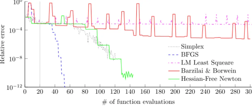
By using different optimization algorithms to minimize the unedited objec-tive function, figure 1.2 is created. The figure shows the function evaluation output against the number of performed function evaluations for all different optimization algorithms. Because the optimal function output is computed by comparing the actual image with a virtual one, the minimum objective function is generally not zero but an unknown arbitrary number. The number itself is insignificant other than that when it is minimized the candidate solution should be a good approximation to the actual solution.

Since the error starts relatively large but get quite small after a few iterations, a logarithmic scale has the advantage of showing both behaviours in a single plot. And since the function output is a arbitrary number anyway, all results are shown relative to the lowest found function output. These relative errors are shown in figure 1.2.

0 20 40 60 80 100 120 140 160 180 200 220 240 260 280 300 10−12

10−8 10−4 100

# of function evaluations

Relativ

e

error

Simplex BFGS

LM Least Squeare Barzilai & Borwein Hessian-Free Newton

Figure 1.2: Relative error vs the number of function evaluations for different optimization algorithms.

(11)

0 2 4 6 8 10 12 14 16 18 20 22 24 10−4

10−3

10−2

10−1

100

Relativ

e

error

Simplex BFGS

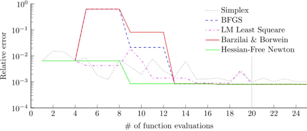
Figure 1.3: Relative error vs the number of function evaluations, showing the relevant interval.

1.4 Objective function analysis

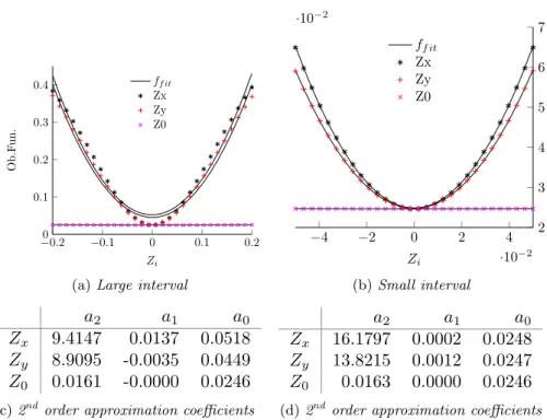
To gain insight in the behaviour of the objective function close to the optimal coordinates. For each coordinate one coordinate is varied while the other two coordinates are fixed in their optimal position. The results of these experiments are shown in figure 1.4. Subfigure 1.4a shows that there are only subtle difference between the two angular dimensions while there is a large scaling difference between the angular and distance variables.

(12)

−00.2 −0.1 0 0.1 0.2 0.1

0.2 0.3 0.4

Zi

Ob.F

un

.

ff it Zx Zy Z0

(a)Large interval

−4 −2 0 2 4

·10−2

2 3 4 5 6 7

·10−2

Zi

ff it Zx Zy Z0

(b)Small interval

a

2

a

1

a

0

Z

x

9.4147

0.0137

0.0518

Z

y

8.9095

-0.0035

0.0449

Z

0

0.0161

-0.0000

0.0246

(c)2nd _{order approximation coefficients}

a

2

a

1

a

0

Z

x

16.1797

0.0002

0.0248

Z

y

13.8215

0.0012

0.0247

Z

0

0.0163

0.0000

0.0246

(d)2nd _{order approximation coefficients}

Figure 1.4: Function evaluation for one dimensional changes and their polynomial fit

1.5 Objective function scaling

Generally in optimization an optimizer will convert quicker if the objective func-tion is smooth, convex and well condifunc-tioned. As previously menfunc-tioned, the ob-jective function close to the optimal value can be described with a second order polynomial function. This means it is smooth and convex. However, as the coefficients of the angular and the distance dimensions are orders of magnitude apart, the objective function is not well conditioned. This results in reduced performance as the gradient in theZ0 direction will initially be smaller and the value will not improve until the other variables are close to their minimum and all gradients are similar. To improve the convergence rate it can be beneficial to precondition the objective function in such a way that it is more symmetrical.

Equations (1.12) and (1.13) describe how a scaling factorS is determined. With a root finder the input that will produce the same function output at point his determined so that equation (1.12) holds. This value ˆxis converted into a scaling factor for each dimension using equation (1.13). The goal is to scale all three approximated objective functions by pre-multiplying the input

(13)

ˆ

fi(x) =a0+a1x+a2x2 fori=x, y,0 (1.11) ˆ

fx(h) = ˆfy(ˆxy) = ˆf0(ˆx0) (1.12)

Si=

ˆ

xi

h (1.13)

f(h)∼f(S2h)∼f(S2h) (1.14)

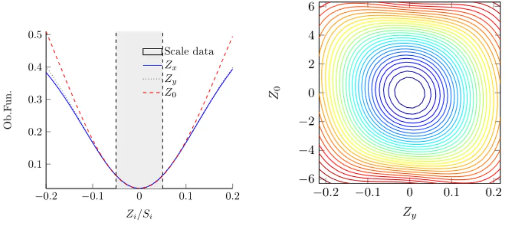
The results of this scaling is shown in figure 1.5a, the highlighted area marks the domain of the input data that is used to determine the scaling factor. Out-side this area theZ0dimensions starts to diverge from theZxandZydimensions,

but they are still of a similar order of magnitude. Figure 1.5b shows a contour plot that shows the objective function for Zy andZ0, this shows the same

be-haviour as the one dimensional plots, but also shows that the objective function transitions in a smooth way from one dimension to the other.

−0.2 −0.1 0 0.1 0.2 0.1

0.2 0.3 0.4 0.5

Zi/Si

Ob.F

un

.

Scale data

Zx

Zy

Z0

(a)One dimensional behavior

−0.2 −0.1 0 0.1 0.2

−6

−4

−2 0 2 4 6

Zy Z0

(b)objective function versusZ0 andZy

(14)

1.6 Improvement analysis

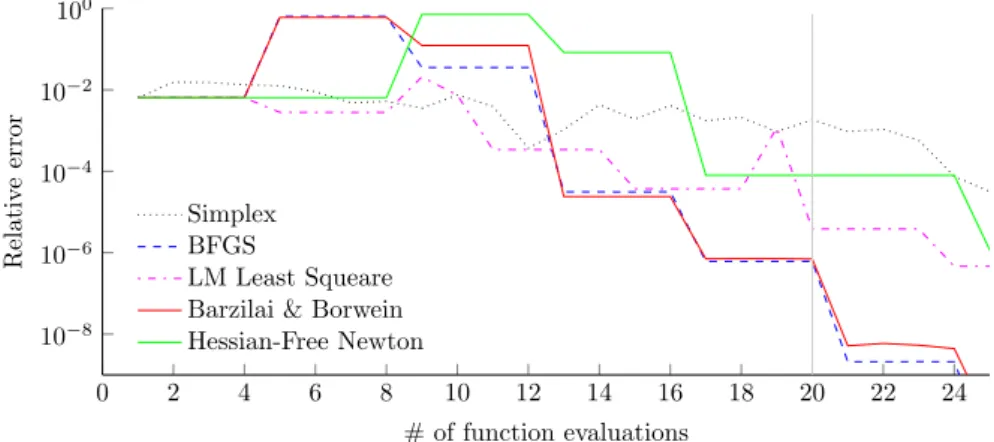
To test if the scaling of the objective function has improved performance, the relative error is plotted against the number of used iterations in figure 1.6 in the same way as was done in section 1.3. Without the preconditioned objective function, the initial error ofO(−2) was reduced to orderO(−3) in 20 function calls. Using the preconditioned objective function, the error after 20 function calls ranges fromO(−3) toO(−6.5) depending on the used optimization scheme. The procedure for the next analysis is to run 30 randomly generated start points that are relatively close to the optimal coordinates Si. This is done for

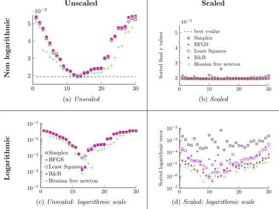
both the unconditioned and conditioned cases (1.7a and 1.7c vs 1.7b and 1.7d). The results showed are sorted on the output coordinate of theZ0dimension to make a particular behaviour of the optimizers more clear. Apparently the

Z0 dimension is the main contributor to the final error output in the unscaled cases. Sorting only that dimension creates an orderly result with the minimal error at the middle of the spectrum. The reason for this is that the optimizer first optimize for the other dimensions as these gradients are orders of magnitude larger than theZ0direction, leaving theZ0coordinate close to the initial random location. The same behaviour holds true to some extend for the scaled objective functions, but this time around there are more examples of a larger error inZ0 direction that result in a lower overall error. Combined with the generally lower objective function output this suggests that the Z0 direction is still the main contributor to the output error. But it is closer to the level of error in the other directions and that the general performance has increased significantly.

0 2 4 6 8 10 12 14 16 18 20 22 24

10−8

10−6

10−4

10−2

100

Relativ

e

error

Simplex BFGS

(15)

Unscaled Scaled

Non

logarithmic

0 10 20 30

2 3 4 5

·10−2

(a)Unscaled

0 10 20 30

2 3 4 5

·10−2

Sorted

final

y

v

alues

best yvalue Simplex BFGS Least Squares B&B

Hessian free newton

(b)Scaled

Logarithmic

0 10 20 30

10−5

10−4

10−3

10−2

10−1

Simplex BFGS Least Squares B&B

Hessian free newton

(c)Unscaled: logarithmic scale

0 10 20 30

10−7

10−6

10−5

10−4

10−3

10−2

Sorted

logarithmic

error

(d)Scaled: logarithmic scale

Figure 1.7: normal and logarithmic scaled error for the same 30 random start values between −0.05·Si and0.05·Si of the optimal point using different

(16)

1.7 Image Series

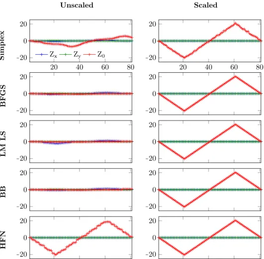
To test the optimizers in an actual application, a series of 120 images is analysed. These images were captured during the movement of an actuated mechanical arm. In this case the arm rotated around the Zx axis maintaining the same

position in the other degrees of freedom. These images were analysed after the fact using the different optimization algorithms both with and without a one time scaling procedure.

As the exact coordinates of each image are not known, the performance has to be measured in an indirect way. The sum of all objective functions output over the series is shown in table 1.8 and the estimated output coordinates are displayed in figure 1.9. The values is table 1.8 are fairly large compared to the differences between methods. This is because a large portion of these values is composed of differences between the actual image and the virtual rendering.

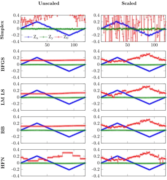
Comparing the results show that the simplex method has the worst perfor-mance across the board. Contrary to the random initial points the accuracy decreases when using the scaling factor. The images in figure 1.9 show a possi-ble explanation for this. As the results ofZ0are better in the scaled version, the accuracy of the other dimensions seems to deteriorate. The other methods do not seem to exhibit this behaviour and show slightly improved accuracy. Also, the performance of all 4 methods seem to be an improvement over the Simplex method. Although the scaled BB method has the best numerical results, the differences are so small that they all seem like viable options. In other situations or using slightly different parameters, the other algorithms could prove to be superior in that scenario.

Looking at the images of figure 1.9 it seems like the most critical degree of freedom is the Z0 direction as was expected by the previous experiments. Another thing that is unexpected is that there is a structural variation in the

Z0 direction in the scaled experiment. Since all but the Simplex method shows the same behaviour, it is likely not a optimization problem but a calibration error or an unintentional variation that occurred while creating the images.

As theZ0dimension is the most critical direction, that behaviour is dominant to the overall performance of the system. When looking at figure 1.10 it seems like the noise is significantly lower than that of figure 1.9. Note however that due to scaling the figure’s y-axis is about 60 times larger as the previous images so the noise is still there. It does show that all but the Hessian Free Newton method can not detect the large variation in Z0 direction, while in case of the scaled objective function they can. Another observation is that in the unscaled o.f. there is an interaction between the dimensions, as all variables except the

Z0 coordinates are kept constant and with certain methods the Zx direction

changes. This can either be because of the earlier mentioned calibration error or because there actually is a interaction.

(17)

Algorithm Unscaled Scaled

P

f(xf in) ∆ Pf(xf in) ∆

Simplex 6.183 0.149 6.490 0.458

BFGS 6.043 0.010 6.032 1.45·10−5

LS 6.055 0.022 6.045 0.013

BB 6.043 0.010 6.032

-HFN 6.033 - 6.034 0.003

Figure 1.8: Total objective function of all images and the difference between the best and current algorithm

Unscaled Scaled

Simplex

50 100

−0.4

−0.2 0 0.2 0.4

Zx Zy Z0

50 100

−0.4

−0.2 0 0.2 0.4

BF

GS

−0.4

−0.2 0 0.2 0.4

−0.4

−0.2 0 0.2 0.4

LM

LS

−0.4

−0.2 0 0.2 0.4

−0.4

−0.2 0 0.2 0.4

BB

−0.4

−0.2 0 0.2 0.4

−0.4

−0.2 0 0.2 0.4

HFN

−0.4

−0.2 0 0.2 0.4

−0.4

−0.2 0 0.2 0.4

Figure 1.9: Z output values using different algorithm for a series of real images with variable Zx coordinates. The left and right columns use respectively the

(18)

Unscaled Scaled

Simplex

20 40 60 80

−20 0 20

Zx Zy Z0

20 40 60 80

−20 0 20

BF

GS

−20 0 20

LM

LS

−20 0 20

BB

−20 0 20

HFN

−20 0 20

Figure 1.10: Z output values using different algorithm for a series of real images with variableZ0 coordinates. The left and right columns use

respectively the unscaled and scaled objective function.

Algorithm Unscaled Scaled

P

f(xf in) ∆ Pf(xf in) ∆

Simplex 34.505 31.507 2.347 0.3341

BFGS 39.657 36.659 2.013

-LM LS 37.999 35.001 2.014 0.0003

BB 39.426 36.428 2.014 0.0003

HFN 2.998 - 2.021 0.0082

(19)

1.8 Virtual image series

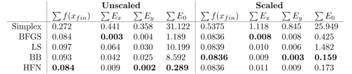
Since the exact coordinates of the real image series are not known, the exact error can not be measured directly. To be able to quintify the error in every independent degree of freedom, a virtual image is used instead of the camera input. Using the code that creates the virtual images in the objective function, a series of images with similar properties to the actual images is created. This way all the coordinates are known and the cumulative error for each degree of freedom can be calculated. If the results of these experiments match the observation of the actual images, this method can in some cases be used as an alternative to the series of actual images.

The results of the virtual image series experiments are shown in tables 1.12, 1.13 and 1.14. Also the coordinate plots are shown in the appendix in figures A.13, A.14 and A.16.

A difference with the actual images is that the objective function output approaches zero instead of an arbitrary number and, as was mentioned before, with this method the error in the various dimensions can be calculated exactly. When comparing the results of the virtual series of figure 1.15 with the actual results of figure 1.9 all behaviours are similar except the behaviour that is al-located to a possible calibration error. This suggest that results from virtual experiments are representative of actual behaviours, although more experiments might be necessary to confirm if this holds true for other applications.

Unscaled Scaled

P_f₍_x

f in) PEx PEy PE0 Pf(xf in) PEx PEy PE0

Simplex 0.272 0.441 0.358 31.122 0.5375 1.118 0.845 25.949

BFGS 0.084 0.003 0.004 1.189 0.0836 0.008 0.008 0.425

LS 0.097 0.064 0.030 10.199 0.0839 0.010 0.006 1.482

BB 0.093 0.042 0.025 8.592 0.0836 0.009 0.003 0.159

HFN 0.084 0.009 0.002 0.289 0.0836 0.011 0.009 0.173

Figure 1.12: Results from virtual generated images where only Zx changes.

Unscaled Scaled

P_f₍_x

Simplex 2.32 0.740 0.735 115.52 0.4405 0.687 0.764 33.0522

BFGS 4.51 0.856 0.593 168.00 0.0835 0.009 0.007 0.110

LS 15.52 3.223 1.139 331.98 0.0839 0.042 0.031 0.394

BB 16.34 3.383 1.048 345.46 0.0835 0.008 0.002 0.072

HFN 0.10 0.075 0.051 6.35 0.0836 0.010 0.005 0.544

(20)

Unscaled Scaled

P_f₍_x

Simplex 0.653 0.447 0.601 46.219 0.48664 0.973 0.926 22.472

BFGS 2.325 0.509 0.380 119.069 0.083811 0.008 0.006 0.191

LS 2.242 0.517 0.410 115.133 0.085310 0.061 0.087 0.519

BB 2.251 0.499 0.373 116.310 0.083817 0.010 0.003 0.225

HFN 0.090 0.040 0.031 4.731 0.083817 0.009 0.004 0.150

Figure 1.14: Results from virtual generated images where all variables are changed over time.

Unscaled Scaled

Simplex

50 100

−0.2 0 0.2

Zx Zy Z0

50 100

−0.2 0 0.2

BF

GS

−0.2 0 0.2

LM

LS

−0.2 0 0.2

BB

−0.2 0 0.2

HFN

−0.2 0 0.2

(21)

Chapter 2

Program guide

For anyone working with the created program, either to implement it in an application or to replicate the results, it is useful to know the global layout of the program and the different processes and their role. A schematic representation of this is shown in figure 2.1. The program is split in two general components, a Setup stage that only has to be executed once and is used to calibrate the hardware and to scale the objective function. Since these operations are only executed once, they are not optimized for speed nor restricted in the number of operations.

After this setup stage, the actual Operation stage can commence. In this stage first the initial coordinates are determined, this is also a one time operation and generally takes longer than the analysis of a single image. This step is just the analysis of a single image but since the initial error is larger than the during operation, the optimization algorithms need more function evaluations and possibly a more aggressive filter. Once the initial coordinates are found the error is typically rather small as the location is corrected every 5 ms and the algorithms should be able to correct the error in only 20 iterations. Every 5 ms a new image is loaded into the algorithm with the previous coordinate data as initial coordinates for the algorithm.

2.1 User interface

The user interface is composed out of two elements, there is a ’Dashboard’ in the root program where certain information is stored like the file name of the images, the range of analyzed images and config file names. Besides this dashboard the program requires the user to navigate a series of menus to select the operating mode.

2.1.1 Dashboard

(22)

two images image coordinates

config file Calibrate

Optional: Scaling

Find initial coordinates

Find coordinates

current coordinates image

updated config

scaling factor

xinit

Setup stage

Operational stage

xinit

Figure 2.1: Program

2.1.2 Graphical user interface

The menu structure of the GUI is shown in figure 2.2.

Use last Settings

This menu lets the user choose the last used settings to circumvent the under-lying menus, this only works if the previous run was completed without errors as the settings are only saved at the end of the program.

Choose Mode

Calibrate: At the moment this option is empty, but it is intended to be used for a calibration algorithm that will determine the geometry parameters of a particular setup and updates the config file with this information.

Find scaling factor: This option directs to the code used to find the scaling factor as is described in section 1.5. Yes: This option uses a previously calculated scaling factor and checks the quality of the fit. It will produce a graph that shows the scaled objective function on a large data range to assess the goodness of fit for coordinates outside the data range that was used to determine the fit.

No: If the existing scaling factor is not chosen it will create a new scaling factor, using a few hundred function evaluations andfac overwriting previously found factors. unscaled: used for image 1.4, scaled: image 1.5a

Image Series: The core of the program, this is the actual application of the code, It asked if it should use the scaling factor and it gives the option to select an optimization algorithm or loop over all five algorithms. used for images 1.9, 1.10, 1.15, A.13, A.14, and A.16

(23)

Choose experiment

Benchmark: Creates a figure for the time it takes to calculate 1000 function evaluations and virtual images, this isn’t mentioned in the report.

Random points: Creates a figure of the output coordinates of a single image for multiple starting positions for all optimization algorithms. used for images of figure 1.7

Iterations vs. error: Shows how the objective function varies over an increas-ing number of function evaluations for the different optimizers. used for images 1.2, 1.3 and 1.6

2d surface: used for images 1.5b

Basic optimizer: Finds the best coordinates withnmax function evaluations

for a single image using the chosen optimizer.

Use last settings

yes

no

Choose Mode

Calibrate

Find scal-ing factor

Use predefined scaling factor?

No % Find scaling factor

Image Series

Yes % Test scaling factor over a larger area

Use predefined scaling factor?

Yes

No

% Calibrate camera, not yet implemented

Choose optimization algorithm

Simplex

BFGS

LM LS

BB

HFN

Loop over all

-Experiments-% Use the same settings as the previous run

% Loop over all 5 algorithms % Requires Matlab 2011a? or higher Choose experiment

Benchmark

Random points

Iterations vs. error

2D surface

Basic optimizer

(24)

Appendix

A.1 Coordinate plots

Unscaled Scaled

Simplex

20 40 60 80

−20 0 20

Zx Zy Z0

20 40 60 80

−20 0 20

BF

GS

−20 0 20

LM

LS

−20 0 20

BB

−20 0 20

HFN

−20 0 20

(25)

Unscaled Scaled

Simplex

50 100

−5 0 5

Zx Zy Z0

50 100

−5 0 5

BF

GS

−5 0 5

LM

LS

−5 0 5

BB

−5 0 5

HFN

−5 0 5

Figure A.14: Virtual series of images with a ∆Z0 of 0,2.

Unscaled Scaled

P

f(xf in) PEx PEy PE0 Pf(xf in) PEx PEy PE0

Simplex 2.32 0.740 0.735 115.52 0.4405 0.687 0.764 33.0522

BFGS 4.51 0.856 0.593 168.00 0.0835 0.009 0.007 0.110

LS 15.52 3.223 1.139 331.98 0.0839 0.042 0.031 0.394

BB 16.34 3.383 1.048 345.46 0.0835 0.008 0.002 0.072

HFN 0.10 0.075 0.051 6.35 0.0836 0.010 0.005 0.544

(26)

Unscaled Scaled

Simplex

50 100

−2 0 2

Zx Zy Z0

50 100

−2 0 2

BF

GS

−2 0 2

LM

LS

−2 0 2

BB

−2 0 2

HFN

−2 0 2

Figure A.16: Z output values using different algorithm for a series of images. The left and right columns use respectively the unscaled and scaled objective

function.

Unscaled Scaled

P

f(xf in) PEx PEy PE0 Pf(xf in) PEx PEy PE0

Simplex 0.653 0.447 0.601 46.219 0.48664 0.973 0.926 22.472

BFGS 2.325 0.509 0.380 119.069 0.083811 0.008 0.006 0.191

LS 2.242 0.517 0.410 115.133 0.085310 0.061 0.087 0.519

BB 2.251 0.499 0.373 116.310 0.083817 0.010 0.003 0.225

HFN 0.090 0.040 0.031 4.731 0.083817 0.009 0.004 0.150

(27)

Improving convergence of numerical optimizers using a limited number of function evaluations