Three models of the term structure of interest rates

University of Warwick institutional repository: http://go.warwick.ac.uk/wrap

A Thesis Submitted for the Degree of PhD at the University of Warwick

http://go.warwick.ac.uk/wrap/36336

This thesis is made available online and is protected by original copyright. Please scroll down to view the document itself.

Three Models of the Term Structure

of Interest Rates

Joonhee Rhee

Submitted in accordance with the requirements

for the degree of Ph.D.

University of Warwick

Warwick Business School

Acknowledgement

First of all, I wish to express my appreciation to my parents for giving me the opportunity to continue to study. Without their unending love, I could not have completed this thesis. My only anxiety is that for the last three years I may not have been a very good son.

I also wish to thank my supervisor Dr. Nick Webber. I have always been grateful ' to him for his excellent advice and helpful comments, without which my work would

not have progressed.

I also thank Dr. Jack Broyles, who encouraged me whenever I was in despair and whose suggestions were always greatly appreciated

Professor Sang Yong Park of Yonsei University, Seoul, Korea supported me financially and psychologically from the start of my studies. I shall never forget his kindness.

I also thank Mr. Keith Taylor for English corrections of my thesis.

Abstract

In this dissertation, we consider the stochastic volatility of

short rates, the jump property of short rates, and market

expectation of changes in interest rates as the crucial factors in

explaining the term structure of interest rates. In each chapter,

we model the term structure of interest rates in accordance with

CONTENTS

Chapter 1. Introduction

1

Chapter 2. Asset Pricing in Financial Economics:

General Equilibrium and Martingales

6

Chapter 3. The Theory of the Term Structure of Interest Rates

and a Review of the Existing Literature

17

3.1. Introduction

17

3.2. The General Equilibrium Approach

18

3.3. The Risk Neutral Approach

21

3.4. The Affine Model of the Term Structure of Interest Rates

29

3.5. Issues for the Modelling

of the Term Structure of Interest Rates

35

3.6. Conclusion

37

Chapter 4. A Three-Factor Model of The Term Structure

of Interest Rates

38

4.1. Introduction

38

4.2. The Model and Its Derivation

41

4.2.1. The Model

41

4.2.2. Derivation of the Partial Differential Equation

43

4.2.3. The Features of the Model

49

4.3. An Estimation of the Parameters

58

4.4 Conclusion

67

,

Chapter 5. An Affine Term Structure Model with

69

5.1. Introduction

69

5.2. An Affine Model of the Term Structure With Jumps

70

5.3. An Affine Factor Model with Jumps

72

5.4. An Example of an Affine Term Structure model with Jumps

77

5.5. An Estimation of the Two-Factor Jump-Diffusion Model

91

5.5.1. An Approximate Maximum Likelihood Estimation

91

5.5.2. Empirical Results

98

5.6. Conclusion

107

Chapter 6. A Model of Term Structure of Interest Rates

under the Expectation of Regime Changes

6.1. Introduction

108

6.2. Review of Model

111

6.2.1. Cagan-Type Model

111

6.2.2. Rational Expectation Model of Interest Rates

114

6.2.3. Continuous Time Version of the Sargent Interest Rate Model 115

6.2.4. The Sargent-Type Model of Interest Rates

under the Probability Measure Q

118

6.2.5. Structural Framework of BGM

124

6.2.6. Our Model

131

6.3. An Explicit Form for Forward Rates

132

6.5. Conclusion

142

Chapter 7. Summary and Conclusion

143

Appendix I. A Closed-Form Solution of

a Pure Discount Bond Price

146

Appendix

A Determination of A and B

Appendix

Positive Interest Rates in the Presence of Jumps

157

A111.1.

Introduction

157

AIII.2. Review of the Flesaker and Hughston Approach

157

AIII.3. An Extension to Jumps

160

AIII.4. The Pricing of Contingent Claims

164

AIII.5 Conclusion

165

Appendix

Review on GMM Estimation of

the Multi-Factor Diffusion Model

166

AIV.1. Introduction

166

AIV.2. GMM Estimation of the Diffusion Model

167

AIV.3. Example : Two-Factor Model

170

AIV.4. Example : An Algorithm for the Two-Factor Model

172

AIV.5. A Grid Approximation

175

AIV.6. A Generalization of Transformation

in a Multi-Factor Diffusion Model

176

Lists of Tables

,

Chapter 4

Table 1. Base Case of Parameters

Table 2. Comparison of Models

Table 3. Estimates Using the GARCH-X Process

Table 4. Estimates of Annualized Parameters

. Chapter 5

Table 1. Errors Percentage of Interest Rates Difference in Model 1

Table 2. Errors Percentage of Interest Rates Difference in Model 2

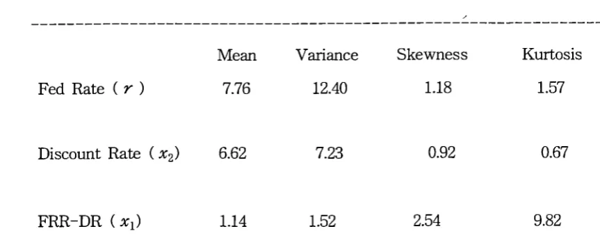
Table 3. Statistics of Data (monthly data)

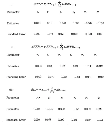
Table 4. Unit Root Test for FFR, DR, and x1

Table 5. Cointegration Test

Table 6. Estimates of Parameters (Bernoulli Mixture Gaussian)

Table 7. Estimate of 7h, 721 and 7

Table 8. Estimates of the Original Parameters

Table 9. Estimates of Parameters for Equation (38)

Chapter 6

Lists of Figures

Chapter 4

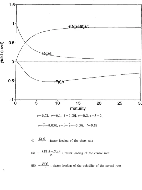
Figure 1. The Term Structure of Interest Rates

Figure 2. Factor Loadings

Figure 1 Interest Rates

Figure 4. Residual

Chapter 5

Figure 1. Interest Rates

Figure 2. Size of Jump of Discount Rate

Chapter 6

Chapter 1. Introduction

The term structure of interest rates plays a pivotal role in financial economics, from a simple NPV (Net Present Value) calculation to advanced options pricing. The interest rate, especially the short rate, is detelinined by complex economic forces. Models of the term structure of interest rates should reflect some, if not all, parts of this complexity. In this dissertation, we consider the stochastic volatility of short rates, the jump property of short rates, and market expectation of changes in interest rates as the crucial factors in explaining the term structure of interest rates. In each chapter, we model the term structure of interest rates in accordance with these factors.

The most natural way to model the term structure of interest rates in finance is to choose a general equilibrium framework. This approach involves a kind of microeconomic problem in a macroeconomic setting. Lucas (1978) and Sargent (1987) follow this approach in pure economics, and Cox, Ingersoll and Ross (1985b) and Longstaff and Schwartz (1992) do so in financial economics. Unfortunately, the approach has some limitations. The spot rate and the price of financial derivatives are expressed as an indirect utility function. When we implement a model from the general equilibrium framework, we have to specify or estimate the parameters of the utility function. Recently, Duffle (1992), Duffie and Epstein (1992) and Duffie and Lions (1992) have directly modelled the utility function in a continuous time framework. Hence they have considerably reduced the inconvenience associated with the general equilibrium modelling. However, they have not resolved all the problems involved in solving the associated Partial Differential Equation and, most importantly, in solving the problem of a utility function in the presence of jumps.

A very significant revolution in finance is represented by the application of martingale theory to check the no-arbitrage condition in pricing financial derivatives

,

or modelling the term structure of interest rates. This step distinguishes finance from economics. If a model of financial derivatives satisfies the no-arbitrage condition, it is not necessary to model in a general equilibrium framework. Harrison and Kreps (1979) obtain this result, and Harrison and Pliska (1981) develop it further. They call this characteristic "viability", which means "always supportable" by a general equilibrium framework.

We apply this latter approach to model the term structure of interest rates in a continuous time framework. Three main aspects of the dissertation will be highlighted

First, we present a three-factor affine model of the term structure of interest rates, in which the factors are the spread rate, its volatility and the long rate. The long rate that we consider in the first case is the consol rate. In the second case, the long rate used is a bench-mark rate affecting the level toward which the short rates converges. In the case of using the consol yield, we extend a two-factor model proposed by Schaefer and Schwartz (hereafter SS, 1984) to a three-factor case. Our model adds the stochastic volatility of the spread rates process. We also provide an approximate solution to the fundamental valuation equation using orthogonal state variables. In a similar context, we use a bench-mark rate affecting a level toward which the short rates converges as a factor. We shall explain this further in Chapter 4. We successfully provide a closed form solution of a pure discount bond price, using three factors in the latter case.

Thirdly, we investigate a model of the term structure of interest rates in the presence of expectations of changes in the regime of interest rates, or of bubbles.

,

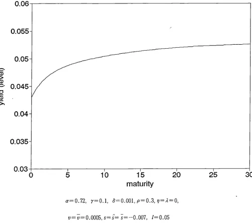
We express the model of the term structure of interest rates in terms of forward rate processes in a similar way to the frameworks of Brace, Gatarek, and Musiela (1997, BGM), and Jeffrey (1994). Assuming a Gaussian and time-homogeneous volatility structure, we present an explicit solution for forward rates in terms of fundamentals l , and consequently for a pure discount bond price under the expectation of changes in regimes. In this procedure, we re-interpret the Sargent (1972)-type interest rate model in the continuous-time framework of modem finance.

The structure of the dissertation is as follows.

In Chapter 2, two approaches to pricing the financial assets are explained: the general equilibrium approach and the no-arbitrage approach (martingale approach). To clarify the concept of the martingale in finance, the martingale measure is expressed in terms of time and state preference. In addition, some important concepts in a stochastic model, such as the Radon-Nikodym derivative and the Girsanov theorem, are explained.

In Chapter 3, we explain the theory of the term structure of interest rates both in the general equilibrium model and the martingale context in Sections 2 and 3. In the general equilibrium context, we explain how to obtain a pure discount bond price and pricing kernel from the the Euler equation. In particular, the pricing kernel approach in finance is quite important because it overcomes the arbitrary specification problems of the market price of risk in the martingale approach. Following Jamshidian (1991), we explain the relationships between spot rate process, forward rate process, and bond price process in the martingale measure context (this relationship is used in Chapter 6). In Section 4, we explain Duffie and Kan's (1996) affine model of the term structure of interest rates. Two chapters of the dissertation (Chapters 4 and 5) are in fact based on the affine framework. We also review affine

1. We shall provide a formal definition of the fundamental in Chapter 6.

-type models of the term structure of interest rates, such as that of Fong and Vasicek (1991). In Section 5, we explain how the three main Chapters 4, 5 and 6 can be integrated as one topic. The empirical distribution of changes in interest rates displays the leptokurtosis of interest rates. The distributional kurtosis can be explained by stochastic volatility (Chapter 4), the jumps of interest rates (Chapter 5), and the market expectation of interest rates (Chapter 6).

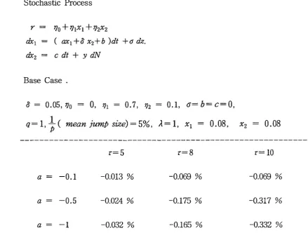
In Chapter 4, we investigate a three-factor affine model of the term structure, assuming stochastic volatility. We present an approximate solution of a pure discount bond price and a closed form solution of a pure discount bond price. Two models are examined. In the first model, the drift term of the consol rate is derived from the no-arbitrage condition. In the risk-neutral measure, this model is not an affine model. To obtain an approximate solution of a pure discount bond price, we assume that the drift term of the consol rate is linear with respect to the consol rate. In the second model, we use a long-term rate which affects the convergence of short rates as a factor. We successfully provide a closed form solution for a pure discount bond price. In an empirical estimation, our model is discretized in terms of a GARCH-X specification. In addition, we compare the model with Schaeffer and Schwartz's (1984) model, using the LR test.

In Chapter 5, we extend the affine model of the term structure of interest rates to the presence of jumps. We also present an approximate solution of a pure discount bond price in a two-factor case. First, we show how the affine framework can be extended to the jump diffusion case. In the next section, as examples, we demonstrate the two-factor jump-affine model of the term structure in two cases and obtain approximate solutions. In an empirical estimation, we use a maximum-likelihood method for the approximate density.

economy model is known to be viable in this sense. It is well-known, however, that the IS-LM model cannot be compatible with a Lucas-type economy. To reflect this, in Chapter 6, we combine the rational expectations model from monetary macroeconomics with a modelling of the term structure of interest rates. In Section 1, we explain the motivation of this chapter. In Section 2, we explain the Cagan-type monetary model, the Krugman and Miller (1992) target zone model, the Sargent-type interest rate model and the BGM model. We demonstrate how the Krugman and Miller framework can be applied to the Sargent-type interest rates model. We express the model of the term structure of interest rates in terms of the BGM framework. In Section 3, we choose a bubble path as a solution.

To obtain tractability or a closed form solution for interest rate derivatives, we sometimes permit the interest model to allow negative interest rates: for instance, the Gaussian model and our two-factor jump-diffusion model. In Appendix lII, we construct a theoretical model of the term structure of interest rates in the presence of jumps to see what kinds of term structure model do not allow negative interest rates. Following Flesaker and Hughston (1996), the interest rate positivity property is incorporated into the discount bond price.

-Chapter 2. Asset Pricing in Financial Econornics:

General Equilibrium and Martingales

Uncertainty in financial economics plays a pivotal role in deteiiiiining asset pricing. If there is no uncertainty, asset pricing is very simple. For instance, in the discrete time framework under certainty, any asset price is just a summation of known discounted future cash flows. In reality, however, the future cash flows and discount factors are unknown. So, how can we reasonably reflect uncertainty in modelling asset prices? The straightforward way to do this is to assume uncertainty in the form of a probability density. Modelling uncertainty as a normal distribution (Gaussian) is the usual approach in financial economics as well as in econometrics. There are several reasons for doing this. The uncertainty can be represented as symmetric about the mean. More fundamental is the advantage of analytical simplicity. Both the unconditional and conditional densities of the normal distribution are normal distributions. In addition, it is rather easy to extend a model to the multivariate case. For instance, when we analyse the relation between the risk premium of the market portfolio and the investors' optimal portfolio decision, we can use Stein's lemma. 2 However, this can be applied only to the normal distribution. Unfortunately, however, the normal distribution assumption does not conform closely to reality. It is well-known that stock returns are more nearly lognormally distributed, and that the underlying stochastic process of this and other economic variables, e.g. interest rates, exhibits skewness and excessive kurtosis

2. Let X and Y be bivariate normally distributed. Then we have

Cov(g(X), Y) = E[g l (X)] Cov(X,Y)

where g is differentiable. This is called Stein's lemma.

(leptokutosis). This means that the distribution is not symmetric and that the return distribution of some assets is fat-tailed. Accordingly, modelling the uncertainty of some assets requires careful attention, and must take into consideration the empirical evidence of the distribution of asset returns.

On the other hand, the continuous-time framework has been a fundamental tool since Merton's (1971) and Black-Sholes' (1973) option pricing. The continuous-time approach is one way of reducing the inaccuracy resulting from the discrete-time approach3. The continuous-time approach has the strong advantage that it expresses uncertainty in the form of a stochastic differential equation instead of as a distribution. Actually these two approaches are the same. In pricing a stock option, the stock price is assumed to follow a lognomal distribution. Equivalently, we could express it as a geometric Brownian motion. When we try to find the density function from the stochastic differential equation, we have to solve the Kolmogorov forward equation. Unfortunately, closed-form solutions are few. In some cases, for instance in Sun (1992), we can to solve a stochastic difference equation. However, solving a differential equation is easier than solving a difference equation. The attraction of the continuous-time approach is mainly due to the simplicity of modelling asset pricing.

One of the most important papers in asset pricing is Lucas (1978), which offers a theoretical examination of the stochastic behaviour of equilibrium asset prices in a pure exchange economy. Lucas investigates the relationship between the exogenously determined productivity changes and market movements in asset prices. Futhermore, he generalizes the martingale property of stochastic asset prices, which is a characteristic of market efficiency (we will discuss the martingale theory in the next section). Lucas models the uncertainty of productivity (in other words, changing the opportunity set) as a probability distribution rather than as a stochastic differential equation. In contrast to Lucas, Merton (1971) derives a relationship

3. Expressing uncertainty in the form of the stochastic difference equation is also possible. Sun (1992) uses a stochastic difference equation approach in analyzing the general equilibrium theory of the term structure of CIR (1985). In his paper, the price formula of a pure discount bond converges to that of CIR (1985).

between the equilibrium expected rates of return on assets in a series of stochastic differential equations. He extends a classical CAPM to the multi-factor CAPM in a continuous-time general equilibrium model. Synthesizing these , two approaches, Cox, Ingersoll and Ross (hereafter, CIR,1985a, 1985b) published a pathbreaking paper. CIR develop a general equilibrium asset pricing model in the continuous-time framework of Merton (1971) and in the Lucas-type economic structure. In OR, the model endogenously determines the stochastic process followed by the equilibrium price of any financial asset and shows how this process depends on the underlying real variables, i.e. for a term structure of interest rates, the economy determines the type of stochastic process for interest rates. This is different from the no-arbitrage approach of term structure modelling used by, for example, Vasicek (1977). One of the principle results of CIR (1985a, 1985b) is a derivation of a partial differential equation which asset prices must satisfy. The solution of the equation determines the equilibrium price of an asset in terms of the underlying real variables.

Asset pricing models must not allow arbitrage opportunities. The papers mentioned above derive asset pricing in the general equilibrium context. This approach automatically guarantees the no-arbitrage condition. In finance, there is another way to derive asset pricing models which does not admit to arbitrage opportunities.

Asset pricing in a general equilibrium context starts from the assumptions of the utility function and a budget constraint. Eventually, we have to solve the Hamilton-Jacobi-Bellman equation. The solution (the investment proportions of the riskless asset and the risky asset) is obtained in terms of an indirect utility function. It requires quite strong assumptions such as a specific utility function and the market clearing condition. The no-arbitrage approach seeks to develop pricing models in an economy with risk aversion and time preference. The no-arbitrage approach assumes only that "people prefer more to less" and is not concerned with the utility functions of individual investors.

in this thesis, we briefly sketch asset pricing in a no-arbitrage economy 4. To explain some concepts in a more intuitive way, we use both a continuous-time and a discrete-time approach throughout this thesis. Assume initially, 1) risk neutral

investors, 2) no time preference, 3) state space 12 with a finite number of states,

4) information structure (filtration), = {Et :t = 0,1 ... 7), E0 = {D}, 5) N+1

securities (the first one is a riskless security), 6) cash flows of security j X; = 1X1(t):t=1 . 7), where j=0, 1.... N+1. Then the ex-dividend

prices S; of a riskless security and the risky securities are

(1) S; = {SP); ,t=1,

So(t) = B(t)

= E(S1 (t+1)+X1 (t+1) 1 EJ

where B(t) is a T-period discount bond with face value equal to one, assuming

that there are no coupons. As the price processes are ex-dividend, B(7)=0,

Following Huang and Litzenberger (1988), we define the accumulated

dividend process for security j to be

4(t)=0X,(s), for all t=0,1...T

Adding DP) to both sides of the third line of (1) gives

(2) S;(t)+D;(t) = E(S1(t+1)+D;(t+1) Iea

= E(S;(s)+D;(s) I )-, for all s > t

where the second line of (2) follows from repeated substitution of the first line of (2)

4. This is based on lecture note of Subrahmanyam (1996) in an EDEN Seminar.

into itself. Thus, in the absence of risk aversion and time preference, prices plus accumulated dividends are martingales. No-arbitrage, therefore, is automatically guaranteed.

Then, what happens when the representative economic agent has a time preference? We can express the asset price in line with the marginal utility of the representative agent5. Then,

U t+i(Ct+i)

(3) B(t) = E( U(C) (B(t+1)) I t

Sp)

for all t < T-1, and where U denotes the utility function, U the marginal utility, and Ct the consumption at time t. As in the expression (3), in the presence of time preference, the spot price is not a martingale, even with the assumption of risk neutrality. To make the spot price a martingale, we rewrite (3) as

(4)

U t-Fi (Ct+ i ) E(U t+i(Ct+i))

I S•(t) = _{t+i(Ct+i)) U t(Ct)} (S1(t+1)+X1(t+1))

Defining,

td-1( 0( t+1)

Ut+I(Ct+1))

where cb is interpreted as a risk adjustment factor. Substituting (5) into (4), we obtain,

E(U t+ i (Ct+ i ) I et) (6) S =

U t(Ct) c5(t+1) (S1(t+1)+X1(t+1)) I et)

5. See Foundation of Financial Economics by Huang and Litzenberger (1988), p. 227.

B(t)

= Bct+i) ) sb(t+1) (s1(t+1)+x,(t+1)) I Et)

Si( t) where the second line of (6) comes from the first line of (3). Let S;(t)=

t)

Xi( t) and X

i

B(t) • For instance, setting N=1, T= 1, then we obtain:

(7) S*(0) = E(.0 (S* (1) + X* (1)) I S2)

= Es2 N-„, (S* (1) + X* (1)).

We define the conditional probability,

(8) z(t) = zw(t)cb,„(t+1)

where 7C is the conditional probability at time t, given the filtration e.t. From (7),

we can obtain the following relationship:

(9) E(

I

=

= Eei

and, using the definition of cb in (5), we find that equation (9) becomes equal to 1.

Hence 7C: behaves like a probability. It is called the Equivalent Probability Measure

(Huang and Litzenbeger, 1988). We rewrite equation (6) as

(10) . S(t) = E(cb(t+i) (S;(t+1)+X;(t+1))

I 0

= E

= E

We obtain an expression in the same form as the third line of equation (1). The security price plus the accumulated dividend are martingales under the new probability measure. Since this measure makes the security price into a martingale process, this probability measure is called the Equivalent Martingale Measure (EMM).

We derive the EMM from the assumption of risk aversion and time preference. However, the security price under EMM behaves like equation (1). Equation (1) is based on the assumption of risk neutrality. Hence the investor is risk neutral under EMM. This is why many authors, including Duffie (1992), call ElVIM the risk neutral measure. However, risk aversion and time preference are captured by the

EMM distribution shift from the original distribution. This martingale measure 7114,

is just the Arrow-Debreu (1954) state price vector. Actually, no-arbitrage is guaranteed if and only if there is a state price vector 6. Since the unique existence of a state price vector means the unique existence of EMM, there is no arbitrage if and only if there exists an EMM. Martingale technology in asset pricing has the same result as the general equilibrium framework but is more straightforward. This is why many asset pricing models are derived from the martingale technology. Harrison and Kreps (1979), Harrison and Pliska (1981), and Huang (1987) are included in this category of authors. However, as Harrison and Kreps point out, financial models from the martingale approach are viable, which means "always supportable" by the general equilibrium model.

How can we be sure of the unique existence of EMM? To understand this, we resort to the Riesz Representation Theorem.

The Riesz Representation Theorem (RRT) 7 : Given a vector space L, with an

inner product defined by (x, = EEmnd x. y I , then for each linear functional

L—>11, there is a unique 71- in L, called the Riesz representation of F, such that,

F(x) = E Emm[ x-- x ] where x E L.

If F is strictly increasing, then 7r is strictly positive.

We show how the RRT can be applied. Following the notation of the existing

literature, we denote the original probability by P and the EMM by Q. As in

Harrison and Pliska (1981), we define a price system for an asset, in particular a

contingent claim, to be a map F. L—>[ 0, C°). Then by RRT, there is a one-to-one

correspondence between the price system F and probability measure Q i.e.,

T

F(X) = E Q(1071 - IX ) As in Duffie (1992), the 7r is called a state-price deflator.

If L is assumed to be dense, then the space L is understood to be a Banach

space8.

The RRT provides the unique existence of EMNI or probability measure Q.

The next problem is how we find the EMM or probability measure Q. To understand this, we need two mathematical concepts: Radon-Nikodym derivatives and the Girsanov Theorem 9. We first introduce the Radon-Nikodym Theorem.

Theorem (Radon-Nikodym)io: If the EIVIM Q is absolutely continuous with

respect to the original probability measure P, then there is a non-negative random

variable p such that for any A E E, Q(A) = 1A pdP. The random variable p

is unique with P-probability one.

The random variable p is called the density of the probability measure Q with

respect to probability measure P, or the Radon-Nikodym derivative of Q. We

8. Banach space is a complete normed vector space. 9. See Dothan (1990), p. 208.

denote this by p = dd(123 11 , Actually, since the Radon-Nikodym derivative p is a kind of likelihood ratio, it should not deviate away from 1 if the two probability measures are to be equivalent. In the preceding theorem, if, for instance

E(p) = 1, then we can create an EMM Q from the original probability measure P

by defining Q(A) = E(1AP) for any event A where l A is a characteristic

function, i.e. if event A happens, then 1 A = 1, otherwise, l A = 0. Then, for any

random variable X, EQ(X) = Ep(pX) and the condition Q(A) > 0 is satisfied

whenever P(A)>O, and vice versa. Futhermore, the probability space should be

equivalent. This means that P and Q have the same events of probability 0. Intuitively, for instance, when today's stock price is E 1, getting, say, E 1000

tomorrow is very improbable. If the probability of £1000 is 0 under probability P,

it is also 0 under Q. Generally, if 9 is a sub-information set of e and Q is equivalent to P, then

, _Ep(p)(19) E Q( X

ls) — Ep(p1s)

We are now in a position to state the Girsanov Theorem. The Theorem

provides a martingale process under the new probability measure Q from an original

process under the old probability measure P in a stochastic continuous time process

such as the Ito process. As mentioned above, the new probability measure Q is

an EMM as well as a risk neutral measure. Hence, any processes under Q admit

no-arbitrage opportunities even without reference to general equilibrium.

A more general version and rigorous proof of the Girsanov Theorem is available

in Oksendal (1995). We just apply the result to an la process.

Girsanov Theorem : Let x be an Ito process in lin

(11) dvt = p t dt + 0t dz

where dz is a standard Brownian motion in lid, and where p: J x [ 0, °°)-4

and a: x [ 0, 00)—>rxd. Suppose v is an n dimensional vector process in some

Banach space12 LI such that 6,0t = p t — v, Then there exists an equivalent

martingale measure Q such that

(12) di; = dz t + 0, dt

defines a standard Brownian motion in lid on the probability measure space

(D, Q) and, then

(13) cixt = v t dt + dZs.

Finally, for any random variable .z,

EQ(z) = Ep(P T

(— fia,dzs foteAds) where to t = exp

Intuitively, the Girsanov Theorem states that if we change the drift term of a given

/7-6\ process, then the probability law of the process does not change dramatically. As mentioned above, the probability law of the new process is absolutely continuous with respect to the law of the old process (by Radon-Nikodym). Futhermore, the new process is a martingale process.

Chapter 3. The Theory of the Term Structure of Interest Rates

and a Review of the Existing Literature

3.1. Introduction

Prior to the development of the general equilibrium approach or the risk-neutral valuation technique (martingale approach), the theory of interest rates seems to have been derived primarily from portfolio theory or basic asset pricing. For instance, Stiglitz (1970) obtained the demand for financial assets and bonds in one-and two-period equilibrium models.

3.2. The General Equilibrium Approach

We will start with the Euler equation, which is similar to the result in Chapter 2, but slightly different in terms of the notation and the asset type. In a standard setting, as presented in Samuelson (1969), Merton (1971), Rubinstein (1976), Lucas (1978) and Breeden (1986), representative economic agents are assumed to base their consumption and portfolio selection on the maximization of the sum of time additive

— —

expected utilities of consumption at each time t in known state co, u(ct, co ). A

necessary condition for an interior maximization at time t is that the decrease in an

agent's satisfaction from selling a marginal pound's worth of assets at t and thereby giving up expected future consumption, must equal the increase in marginal utility from consuming the proceeds at t. Assuming that the sold asset is the T maturity bond at price P(t, T, co ), then the marginal increase in satisfaction of consuming the proceeds from the sale is P(t, T, co)zi (ct, co), where u"(.) is the marginal

utility with respect to consumption. The expected loss in utility from selling the bond is the expectation of its liquidation value P(t+1, T, co) at t+1, times the

marginal utility from consuming the uncertain proceeds u' (c +1 , co) at time t+1.

Mathematically, this can be expressed as

P(t, T, -co)zi (ct, co) - = 1 P(t+1, T , co)u" (ct+1, (071{60)&1) w E sz

where 2r( w) is the probability density function of state co at time t+1, and 9 is the

set of all states. By definition, assuming that { w } is an ordered set, for instance, the real numbers, then the density 7C is given by

a, — \

Pr ob( _{co td-i}(01(0 t = co ) = Lx-(11,

_

w )du.

We suppress the notation dependency on co. We define CP, t+1, a)) = uf ( ct+i, w)

74, (c t, —a)) , which can be interpreted as the price at which, at

the margin, time t consumption in state co is traded off against time t+1 stochastic consumption. The definition of cb u, here is different from that in Chapter 2. Using the definition of O w , equation (1) can be rewritten as

(2) P(t, T, co) = fi,v e j cb,,(t, t+1, w)P(t+1, T, co) ] 7r(co)da) .

This is what we call the Euler equation. We define

x* (co) = q5,(„( t, t+1, co )7r(a))

where 7r* is non-negative and L . s27r* (a)) dco = 1. Since 7r* ( W) can be regarded

as a probability measure, we can write

(3) P(t, T, a)) = E,[ P(t+1, T, co)] .

The transformation from probability measure 7/- to ,r*, which makes the discount bond price a martingale as seen in (3) under the new probability measure, is relatively straightforward in the case of the Von Neumann-Morgenstern utility function. The transformation involves just weighting the probability z of each outcome by the marginal utility of wealth O w ( t, t+1, co) of that outcome.

_

To find a risk neutral measure, we define Y( t, co) to be the one-period riskless _

(4) P(t, T, co) — y(t, (7 1 )) L sl U -00,P, t+1, co)P(t+1, T, (0) ] Y z( co) cico

We define a new measure

7r** (w) = c 6 .2r(w)Y(t, w)

then, from (4)

(5) Y(t, w) -- E 7,4 P(t+1,T, w) i

P(t, T, 0.))

-That is, the bond's expected return computed using the probability measure r** , just

as it would be if investors were risk neutral, equals the riskless return. The .4,

measure 7C is called the risk neutral measure.

To explain the concept of the pricing kernel, the pricing formula (5) can be expressed under probability measure A- as

(6) P(t, T, w) =--- E,[ 61. ,,P(t+1, T, co) ] .

Dividing both sides (6) by P(t, T, a.)) gives

(7) 1 = E[ 0 P:]

where P:, = P(t+1,T, (0)

P(t, T, co)

these models, the real bond yields are positively related to production and consumption growth rates, and are negatively related to uncertainty about future production opportunities. On the other hand, Constantinides (1992) proposed that the

O w, which is called the pricing kernel (we call this approach the semi-equilibrium

approach), should be modelled directly as a stochastic process. This definition is slightly different from that of Sargent (1987), who defines the pricing kernel as

cb z( w) 13 Das and Foresi (1996) follow the pricing kernel approach in deriving a

one-factor jump-diffusion model of the term structure of interest rates. As Constantinides (1992) points out, the direct time-series representation for the pricing kernel makes the procedure of equilibrium specification unnecessary.

This is the main framework of the term structure model of interest rates in the general equilibrium setting.

3.3. The Risk Neutral Approach

Instead of modelling the term structure of interest rates in the general equilibrium context, we can directly model any asset price under the risk-neutral measure or martingale measure. This implies that pricing modelling can be considerably simplified. If we try pricing an asset in a general equilibrium setting, we have to define a utility function and budget constraint, etc. However, as Duffle (1992) pointed out, a martingale is a black box, which makes specifying these unnecessary.

In this section we explain the modern framework of the model of the term structure of interest rates in the continuous-time setting. We also express the term structure model in accordance with the HJM (1992) framework. For simplicity we confine the story to a single-factor Gaussian model in which the uncertainty is

driven by a one-dimensional Brownian motion. In particular, to simplify our analysis, we consider the process Markovian in some cases. An intuitive extension and application to the multi-factor case is available in Karoui and Lacoste (1992).

To explain three seemingly different modellings of the term structure model of interest rates (see equations 9-1, 9-2, and 9-3), we start with some notation. Let

P = P(t, 7-) and f = A t, 7') be the price of a T maturity zero coupon bond at

time t and the instantaneous forward rate at time t, respectively. Then the following relations are true:

P(t, T.) = exp(— ft Tf( t, s)cis )

.gt, 7) = —a[ 1nP(t, TA

a T

P(t, 0 = 1, 7( t) = At, t)

where r(t) is the spot rate. We assume that the instantaneous spot rate, the drift and volatility of bond price, and the market price of risk which shall be defined later are state-independent.

Assuming that the bond price, forward rate and short rate follow /to processes, then:

dP

(9-1) _P — p(t, rdt — o(t, 7) dz

(9-2) df = a(t, T) dt + v(t, r dz

(9-3) dr = a(t)dt + v(t) dz,

following the conventional notation for bond price process, we take minus sign in the diffusion term in equation (9-1). Using /a's lemma, the following relations are satisfied:

(10-2)

(10-3)

(10-4)

(10-5)

a(t, = 1'U'_{a T} + v(t, Tmt, T),

v(t) v(t, t), oKt, = 0, and

= 7(t) — a(t, s)ds cr(t7-)2 .

a(t) — fitaT IT=t — v(t)A(t)

where A(t) is the market price of risk. Equation (10-4) is obtained by integrating

equation (10-2) with respect to T, and using the fact that o(t,t) = 0 and

it(t, = r(t). The proof is available in Hull and White (1993), and Jamshidian

(1991).

The ratio A(t) — P(to(' 7(t) , which is independent of T for all 0 < t T,

is called the market price of risk. Hereafter, we omit the time t for _{A(t) = A.} Then the pure discount bond price at time t is given by

P(t, T) = Eclexp(— r(s)ds)

where the probability measure Q is a risk neutral measure, and by the Girsanov

Theorem, a'. \ = dz — A dt. Using the money market account B(t)= exp( fo r(s)ds)

as the numeraire14, we can obtain the new process,

Ps (t) = P(t, 7) exp(— fo r(s)ds).

14. Any asset in the model whose price is always strictly positive can be taken as the numeraire. We then denominate all other assets in units of this numeraire. The money market account 9( t), for instance, could be the numeraire. At time t, the bond is worth

P(t,

i3(t) units of money market. We could also use the T-maturity bond as the numeraire.

dP* P*

Since this discounted process follows dP* — (p(t, T)— r)dt— o-(t, rdz, P*

p(t, 7-) = r + c( t, T) A holds if and only if — cr(t, r Hence, the

discounted process is a martingale with respect to the probability measure Q. As Jamshidian (1991) points out, it is usually difficult to evaluate the expected discounted payoff for complex derivatives.

On the other hand, if we can assume that the spot rate follows diffusion (9-3), then using the no-arbitrage condition, we can obtain the fundamental PDE which is satisfied by bond prices or the prices of interest rate derivatives. Vasicek (1977), Brennan and Schwartz (1979), Fong and Vasicek (1991), and our three-factor model which is introduced in Chapter 4 are included in this category. In this approach, the arbitrage-free interest rate model is determined by the spot rate and the market price of risk.

Equivalently, we can express the term structure of interest rates as forward rates in terms of the initial yield curve, the bond return volatility, and the market price of risk (9-2). This approach was first introduced by Heath, Jarrow and Morton (HJM) (1992). To see the HJM framework, the no-arbitrage condition

p(t, r = r + 6(t, r A is applied. Differentiating this condition with respect to

T, then from (10-1) and (10-2), we obtain a(t, r = v(t, r (a(t, r — A) (In

,

particular, A = — a(t) evaluating at T = t)15. Thus (9-2) becomes

V(t)

15. By assumption, the market price of risk A(t) is independent of T. Here we show why two definitions of the market price of risk are equivalent To do this, we find a limit value of . lim P(t' _{0(t, T)}r(t) . To find the value, we use L'hospital rule. Differentiating both the numerator and denominator with respect to T, we obtain

Iiin (a (t, 7)— a(t, 7)v(t, 7))

V(t, 7)

where the numerator comes from (10-3). using _{(Kt, 0 = 0, we can obtain the limit value} a(t, t)

(11) df = v(t, TA (0{4

r

= v(t, TA a(t, 7) dt + dZ's ]

= v(t, T)

where dz— is what we call the forward risk-adjusted probability measure, or T

• -measure defined as

dz = (o. — A) dt + dz = dt + d.Z\ .

Integrating the second line of (11), we find

(12) f(t,

r =

This is the HJM term structure model. As seen above, given the market price of risk, the initial yield curve and the volatility structure determine the arbitrage-free term structure model.

Following Jamshidian (1991), in order to examine the volatility structure, the following two volatility functions are defined:

(13-1) x(to, =

ft:

(13-2) y( to, t, = ft:(0(s,

r —6(s, t))2.

where 0 s to s t T. Assuming coefficients are Markovian, we can obtain the

(14) co., er\ v( t) ( cx s _" _ _{v(s, 6 `} 7-)

' a (s , 6)

,

where 0 s t s T. After rearranging, squaring and integrating (14) with

respect to s, we obtain,

I(6(s, T)— o(s , t))) 2

cis = ( cj(vttT) ) 2 ftt v(s, 62ch.

Hence,

(15) y(to, t, T) = (

c(4 t

r

,x(t

, 0.

since 0( t, T) and v(t) are always assumed to be positive. We can rearrange (14) as,

(16) v(s, t) 2 6(t,

7)

Integrating equation (16) with respect to s, the left side of equation (16) becomes

y(to, t, T)x(to, t). Hence (16) becomes

rt

(17) x(to, t) Y(to, t, 7-) = 10 vcs, o[ (Ks, 7)-0-(s, o] ds.

Cornparing (13) with equation (17), this looks like the Cauchy-Schwartz inequality. The equality holds only if the two parts of the integrand of the right side of (17)

are linearly independent. This implies that for fixed T s T, we can find g( T, T)

such that v(t, T) --- g(T, 7) v( 7). Now let h(7) = g(T, 7) and

q(t) = v(t, 7). Thus we obtain

(18) v(t, 7) = g(t)h(T). '

This is the main result of proposition 2-1 of Carverhill. The above result implies that the volatility structure is a deterministic function, and the spot rate process is Markovian. To examine further the volatility structure from Theorems 2 and 3 of Jamshidian (1991), we can express

v( to, 7)

(19) v(t, 7) = v(t)

v( to, 6 •

This expression is obtained from equation (18). From (c) and (d) in Theorem 2 of Jarnshidian (1991), we can find a function a(7) such that for all 0 t T,

T

V(t, 7) = V(t) exp(— ft a(u)du)

a lnv(to, 7) where a(7) =

• a T

From (12) and (19), we have

(20) At, 7) = f(to , 7) + v(vt('_t)7) f v(s, t)[ a(s, 2) dc + c I . n .

For a spot rate, we have,

t

(12-1) 7( t) = IK to , t) + ft V(S, t)[ u(s, t)ds + a',Z] .

fo r t

(21) v(s, t)di = r(t) — At° , t) — fo v(s, t)o-(s, t)a's . ..,

Substituting equation (21) into (20), we obtain,

_At, r = Ato, 7) + v(vt(, tr (7<t)—fuo, 0 + ft:vcs, a 0(s, 7-) —a(s,t)ds I).

. Finally using (17), we express the forward rate as

(22) .gt, T) = f(to,T) + v(t'_v(6 7) (7(6 —f(to, t) +x(to, t)y(to, t, T)).

To express the spot rate process from (22), differentiating (22) with respect to

T

_T

af( (23) dr( t) — ( to, t)

at + x( t0 , t) 2 + a(t)[ flto, t) — r(t)] ) dt + v(t) di

= (c(t) — a(Mt)) dt+ v(t) di

a f(to , t)

where c(t) = _at + x( t0 , t) 2 + a( t) to, t). Hence, the function a(t) is a

mean reversion parameter for the Gaussian model. As seen in equation (23), the initial forward rate curve controls the trends of the future spot rate. Futhermore, the mean reversion of spot rates is towards the forward rate with a rate of speed equal to a(t) . Finally, integrating and exponentiating equation (22) gives a bond pricing formula similar to that in Merton (1973) and Vasicek (1977).

structure of interest rates are eventually closely related. In the next section, we review the existing term structure models. Since these models are discussed in many papers ( e.g. Strickland, 1994), we simply describe, the term structure model and the available applications instead of offering a detailed explanation.

3.4. The Milne Model of the Term Structure of Interest Rates

We can classify models of the term structure of interest rates in many different ways, for instance in terms of the number of factors, or the underlying framework (the general equilibrium approach and the martingale approach), or, the stochastic process of bond prices, spot rates, and forward rates. Since the illustration of these models is provided in the major textbooks such as in Hull (1993), we will not reproduce the details here. However, since our models of the term structure of interest rates in Chapters 4 and 5 correspond to the affine type model published by Duffie and Kan (1996), we shall briefly explain the affine framework.

The Affine Model of the Term Structure of Interest Rates

An Affine Model is one in which bond yields are affine functions of the underlying dynamic factors. Duffie and Kan's (1996, hereafter DK) affine model of the term structure of interest rates encompasses many interest rates models. DK show that if the bond price takes the form of the exponential-affine

P(X, r) = exp(A i (r) + A 2 (r)" X)

where X is an nxl vector, Mr) is a function, A2 (r) is a column vector of an n

dzt dX, = (aX

t

v l (

x

),

2

o, 0,\ v,

i

where a and I are (n x n) matrices, b is an (n x 1) column vector and

v

i

where, for each

i,

li

_dzt

ingX,

independent (n x n) Brownian increments. Since the yield r) is affine

in X, this is called an affine model of the term structure of interest rates. The

affine class of term structure of interest rates includes the Vasicek (1977), CM (1985b), Longs taff and Schwartz (1992), Fong and Vasicek (1991).

The Affine Yield Factor Model

As Duffie and Kan (1996) make clear, yields at fixed maturities are chosen as factors. This is called an affine yield factor model. On the other hand, any state

process Xt

ciX = p(X)dt

ci(X)dz

which may be unobservable is allowed to be an affine factor, and a change of

variables from the original state factor

Xt

Yt

A( r) +B( r)Xt

Yt —

Let k

=

O and

r)

Xt

can write

dY t

= 1

+

where

ii(Y) =

(

(Y

Duffle and Kan show that this change of variables preserves the affine framework. This is also called an affine yield factor model.

Before DK, Brown and Schaefer (BS, 1994b) analyzed a one-factor and a two-factor affine model of the term structure of interest rates. They transformed the bond pricing formula into forward rates and investigated the relationship between the yield and the interest rate volatility. DR extend the model of BS into the multi-factor case. The advantage of this approach is that the yield can easily be expressed in terms of the covariance structure of its dynamic factors. This means that we can express the affine model as a multi-factor Markov parameterization of an HJM model. In Chapter 4 we shall show how to fit the affine model of the term structure of interest rates into the HJM framework (a three-factor case). Another advantage is that we can transform the state variable of the affine model ( which is possibly unobservable) into yield factors of an affine model (observable). Actually, most non-affine multi-factor models do not allow direct observation of the state variables from the yield curve. Filtering may be useful in this case. However, the affine model of the term structure is easily changed into an affine yield model without the use of filtering. Brown and Schaefer (1994b), for example, estimate the parameters of the two-factor model (assuming the two-factor Vasicek process), using the changes of factors into yields.

(1) Vasicek (1977)

,

The best known model of the term structure of interest rates is Vasicek model.

which is is based on the assumption that the short rate r process is as follows:

dr = a(p— r)dt + adz.

In this specification, a closed form solution of a pure discount bond price and a European type bond option formula (Jamshidian, 1989) are available. Chen (1992) also derives the closed-form solution for futures prices and European options on futures and on pure discount bonds. Unfortunately, this specification of the interest rate process allows negative interest rates.

(2) Schaeffer and Schwartz (1984)

In Chapter 4, we extend this model to the three-factor case. Schaeffer and Schwartz model the term structure model with two factors: the spread rates (short rate - consol rate) and the consol rates. Their model is given by

ds--- a( s— s)dt-FI/Vdz

dl= R(s, 1, Odt+ a-adz

where As , 1, 0 = 62 — sl under the risk-neutral measure.

Strictly speaking, their model is not an affine model of the term structure of interest rates. However, since they use an approximation for the drift of the consol

(3) Cox, Ingersoll and Ross (CR. 1985b)

CIR. assume that the short rate process is as follows:

dr = a(p—r)dt + all rdz.

The short rate can here be guaranteed to be positive. Using this dynamic of the short rate, CIR obtain a closed form for a European call option on a pure discount bond. Longstaff (1993) extends the CIR model, deriving formulas for European call and put options on coupon bonds. Chen and Scott (1992) also show that the OR model can be used to price options on bond futures.

(4) Longstctff and Schwartz (LS, 1992)

Using the framework of CIR, LS develop the dynamics of two factors which are independent of each other:

a'x = (7-84dt + Fcdzi

clY = (7)-03)dt + 5dz2.

The spot rate and the the volatility of the spot rate are given by a weighted sum of the factors:

r = ax + igy

v = a2x + )612y.

(5) Fong and Vasicek (FV, 1991)

FV obtain a closed form for a pure discount bond price under the dynamics of the short rate and the volatility of the short rate:

dr = a(r — r)dt + 5 dz 1

dv = 7( v— Odt + (SV vdz2.

Unfortunately, the short rate can be negative. The closed form solution of an option price on bonds is not available.

(6) Chen (1996)

Chen obtains a closed form solution for a pure discount bond price and for other interest rate derivatives under a three-factor dynamic: the short rate, the short-term mean, and the volatility of the short rate, which are given by:

dr = k( 0— r)dt + Fci-V rdzi

dO = v(t9 — t9)dt + 6\16' dz2

da = p(o. — o)it + 7)\17rdz 3 .

where k, v, p, 6, 6, and 7) are constant.

(7) Das and Foresi (1996)

Das and Foresi model the term structure of interest rates under the assumption of the possibility of short rate jumps. Their model is given by:

dr = a( p — r)dt + adz + ydN.

-where dN denotes the Poisson process with constant jump intensity and y is the

jump distribution. The authors assume that the sizes of jumps follow the exponential distribution. They obtain a closed-form solution of a pure discount bond price. In addition, using the Fourier transformation of the probability distribution of interest rates, they obtain the the price of an option on a bond. Unfortunately, as in the Vasicek model, this model produces negative interest rates depending on the parameter values.

In the following section, we shall explain how the next chapters of the dissertation are related.

3.5. Issues for the Modelling of the Term Structure of Interest Rates

The empirical distribution of changes in interest rates displays leptokurtosis. (Das and Foresi, 1996). This implies that the volatility of interest rates follows a stochastic dynamic. Actually, an ARCH specification of a short-rate process fits the market data well (Steeley, 1990). Many two-factor or three-factor term structure models of interest rates assume that the second factor is the volatility of interest rates, as in Fong and Vasicek (1991) and in the two-factor CIR model. Recently, Chen (1996) obtained a closed form for a pure discount bond price and for a bond option price using a three-factor model with stochastic volatility. The stochastic dynamics of interest rates is regarded as crucial in explaining the empirical distribution of changes in interest rates. We shall study this in Chapter 4.

of the stochastic volatility approach: The kurtosis tends to be smaller as the sampling interval becomes smaller in the stochastic volatility model. In this thesis, we model the term structure of interest rates to reflect these distributional effects. Studies based on the jump diffusion term structure models of interest rates are relatively few compared with those of the diffusion model. We shall extend the DK affine model of the term structure of interest rates to the presence of jumps in Chapter 5.

3.6. Conclusion

,

Chapter 4. A Three-Factor Model of The Term Structure

_,

of Interest Rates

4.1 Introduction

Many model of the term structure of interest rates have either one or two factors, and vary the assumption of the specific type of processes (e.g. square root process or Ornstein-Uhlenbeck process). In a two-factor model, the second factor may be the volatility of an interest rate. The Fong and Vasicek (1991), and the two-factor CIR models are examples of these. Recently, Chen (1996) obtained a closed form solution for a pure discount bond price and for a bond option price, using a three-factor model. However, Chen actually obtained the closed-form solution of a pure discount bond price under the assumption that the short rate followed a Vasicek process, allowing interest rates to be negative.

In this chapter, we develop two three-factor affine term structure models of interest rates. In the first model, the factors are: 1) the spread rate (short rate -consol rate), 2) the volatility of the spread rate and 3), the -consol rate. In the second mode117, the factors are: 1) the spread rate (short rate - long rate), where the long rate is defined to be a bench-mark rate affecting the level toward which short rate converges, 2) the volatility of spread rate and 3) the long rate. All factors have mean reversion. To preclude negative values of the consol rate, of the long rate and of the volatility of the spread rate, these processes are assumed to follow a ClR process. The spread rate, however, is assumed to follow a Vasicek process because negative values should be permitted. Hence, our model is not a non-negative affine model (Pang and Hodges, 1995).

The chosen factors and the number of factors are based entirely on previous empirical studies.

Steeley (1990) finds that three factors possibly determine 95% of the term structure of interest rates. He also finds that the short-term interest rate and the spread rate are characterized by the ARCH effect. This provides a clear evidence of the stochastic volatility of the short rates and spread rates (short rate - long rate). Steeley suggests that the long rate (for level), the spread rate (for the slope), and the volatility of the spread rate (for curvature) might provide a better description of the term structure of interest rates.

the Brennan and Schwartz,...." is quite wrong. First, as seen in the next paragraph, since Schaefer and Schwartz use the consol rate rather than the long rate as a factor, their model does not admit an arbitrage opportunity. However, Brennan and Schwartz model may admit arbitrage opportunities. Secondly, as shall be seen in Appendix I, the use of short rate as a factor implies that the mean reversion level of the short rate is fixed. However, the use of the spread rate as a factor allows the mean reversion level of the short rates to vary as it depends on the long mien. Accordingly, the two models are quite different, and the spread rate is not the redefinition of the short rate.

Actually, the consol rate itself might also be regarded as the bench-mark rate. If the consol rate is used as a factor, however, some care should be taken not to admit arbitrage opportunities. Dybvig, Ingersoll and Ross 19 (1989) and Hogan (1993) have shown that in some cases, including the consol rate as a factor may cause the short rate to fail to have a finite-value solution, and consequently must offer the possibility of arbitrage. However, our model does not include these cases. Furthermore, 18. To see the effect of the long rate on the mean reversion of the short rate, we shall compare two models. Ignoring the stochastic term, we set up two-factor interest model as

Model A

dr= a( b— r)dt, dl=m(c— 1)dt

Model B:

ds= k(n — s)dt, dl=m(c— 1)dt

where r is the short rate, 1 is the long rate, and s= r— 1 is the spread rate. All parameters a, b, m, c,k and n are assumed to be constant. In Model A, the mean reversion level b is fixed.

• On the other hand, if we substitute the long rate equation into spread rate equation in

Model B, we obtain

dr= k( kn+mc (m — k)1_{k r)dt}

Duffie, Ma and Yong (1995) obtain regularity conditions by which the short rate and the consol rate are consistent with the definition of the consol rate as the yield on a perpetual annuity under an equivalent martingale measure. The derivation of the drift term for the consol rate in our model satisfies their regularity conditions, especially their equation (4.31).

The plan of this chapter is as follows. In Section 2, we derive the price of a pure discount bond using our three underlying factors. In Section 3, we provide the empirical results of the three-factor model of interest rates, and we present a conclusion in Section 4.

4.2 The Model and Its Derivation

4.2.1 The Model

Assume that uncertainty is specified by the probability space (S2, E, P) , where

e

is a a-algebra subset of ..(2, and P is the probability measure on An adapted

filtration {

ei t

filtration is assumed to be right continuous and P-complete. We assume the following two three-factor models:

(Model 1)

cis= a( s— s)dt+ 6 dzi

clv=-- 7(v— v) + d`F.Klz2

dl= R(s, 1, Odt+ ollldz3

-(Model 2) _,

ds.---- a( --.9-- s)dt+ 6 dz i

dv ---= Ai; — v) + 8/2;d22

dl = - m(1 — 1)dt+ mil d23

where s= r-1 is the spread, r is short rate, 1 is the consol rate in model 1 and a

bench-mark long rate in model 2, and v is the volatility of the spread rate. We

assume that dz i , dz2 and dz3 are standard Gauss-Wiener processes and in

particular, that dz1 dz2 = pdt in model 1, and other instantaneous correlations between

processes are equal to zero, and Q(s, 1) E C2 ( [ 0 , °°)) i.e. a twice differentiable

function. As in Chen (1996), the assumption of dz1 dz2 = pdt might be not necessary

because the spread rate s and its volatility v are already correlated through the stochastic differential equation for the spread rate. We shall assume that all correlations between the Brown motion are zero in model 2. Using this fact, we obtain a closed-form of solution for a pure discount bond price in model 2 in

Appendix I. For model 1, however, we assume that dz 1dz2

=

and Vasicek. We shall specify R under the equivalent martingale measure. In this

chapter, we explain and derive a pure discount bond price only from model 1. The derivation of a pure discount bond price from model 2 is in Appendix I.

A consol bond is defined here as a bond paying a continuous coupon at a rate

of 1 per period with its value equal to . Our model specifies the spread rate

property. Similarly, the volatility equation of the spread rate also has a mean reverting tendency. The consol rate also follows a OR process but the drift term will be specified under the no-arbitrage condition.

4.2.2 Derivation of the Partial Differential Equation

Under the three-factor description of the term structure of interest rates, it follows from ItS's lemma that the instantaneous return on a bond is given by,

(dP+ cdt)

p = pdt-Odzi+gfclz2+Cdz3

where

P

(2) p= ÷-3(a(s—s)Ps+7(v—v)Pv+ RP1+ I- vP,s + -1 62 vP,,,,+ I- 02 1P 11 + 198vPsy + P t+ c),

(3) 0 ---1/7)-1-13-:;, w= an/7) 13;, C= olri-051-,

where c is a continuous coupon rate and the subscripts represent partial derivatives. Since we are concerned with a pure discount bond, we will set c = 0 in deriving a

PDE.

The signs of 0, V, and C are chosen arbitrarily to correspond to the direction of the relationship between each factor and the price.

An arbitrage argument applied to the equation for bond prices leads to the equilibrium condition:

(4) p= rd-A10 +AO/ -F A3C

where A1 , A2 and A3 are the market prices of risk due to Changes of the spread, the

volatility of the spread rate and the consol rate, respectively. To simplify the pricing formula for a pure discount bond, following Fong and Vasicek (1991), we will

assume that A1 and A2 are proportional to the level of risk

A1=A117)

A 2=71\IT).

To derive the partial differential equation satisfied by the value of all default free bonds, we use the fact that the consol rate is inversely proportional to the price of

1 the consol bond as in Brennan and Schwartz (1982). From P=7

PS =0, Ps, =-0, Pr=0, Pv=0, Prn, =0, P1= 721 Pll== .

Substitution of these derivatives for the consol bond into (2) and (4) yields the following expression for the market price risk of consol rate20

(5) de — A3 art= o-2 — s 1 .

As shall be seen in the PDE (6) of a pure discount bond price, 13—A360 is the

coefficient of P1. We can replace this with a2 —sl, and do not need to specify

either 13 and A3.

The drift term (5) and diffusion term of the consol rate in our model is consistent with the equation of (4.31) in Duffie, Ma and Yong (1995). The authors obtain

—1

20. Since 1 (161

12 + 12 o2

regularity conditions by which the definition of the short rate and the consol rate is consistent with the definition of the consol rate as the yield on a perpetual annuity under an equivalent martingale measure. Under their regularity condition, they show that the consol rate process under an equivalent martingale measure Q is21

dl = (— sl + /3 11A11 2)dt + Adz

where, _{A = _12.}

Since the drift term of the consol rate in our case is also derived from the probability measure Q, in our model the consol rate process conforms to this condition22.

Finally, substitution for p from (2) and for the market price of the consol rate

from (5) into the equilibrium condition (4) yields the partial differential equation satisfied by the value of a default-free bond. Therefore, we obtain the partial

differential equation for a discount bond P = P(s, v, 1, r):

2

1

21. In the original paper, they mistakenly write — Mil 2, in which —₂ cancels out by the coefficient of the second derivative of the consol price.

22. To show this, we derive the consol price process from our consol rate process. First, in our model we know that the consol rate process under Q is

dl = (o2 — sl)dt + arl dz.

Using Ito's lemma, we can obtain the consol price process Y under Q is,

dY = —s dt ₁ a dz

1

n

= (rY —1)dt 6

C".