Endoscopic end effector control using soft actuator

(1)

Endoscopic end effector control using soft actuator

Jorn Jansen

(2)

ii Endoscopic end effector control using soft actuator

(3)

iii

Abstract

The minimally invasive and non-invasive surgery are gradually replacing open surgery thanks to an instrument named endoscope. The significance of using soft actuators is to create a flexible instrument that can re-enact properties of a rigid instrument.

In this study, a modified design of an already existing modular continuum robot, STIFF-FLOP, is presented. The number of internal pneumatic chambers has been increased from 3 to 4 to enable antagonistic actuation.

An open-loop control system is implemented based on changing the pneumatic chamber lengths by controlling the applied air pressure. The use of pneumatic actuation in this open-loop control requires the relation between the applied pressure and the pneumatic chamber lengths. This relation is experimentally obtained on one soft actuator in 2 antagonistic direc-tions and with the use of image software the lengths are extracted. To these results a polynomial curve was fitted. A proof of concept for non-antagonistic bending has also been provided in this study.

The control system calculates the chamber lengths based on the desired rotation and bending, it would then, with the use of the pressure-chamber length relation, determine the required air pressure. Because both the actuated chamber and the non-actuated chamber lengths are included in this relation, the algorithm would compensate the actuated chamber length for any changes in the non-actuated chamber length.

With the use of the passive chamber compensation, the angular error was decreased with an average of 70.1% compared to not compensating. Final angular error (with compensation) results have a maximum of 4.74◦

and 4.31◦

for the left and right bending respectively.

The single section modelling and characterization serves as a basis for a more complex multi section endoscope. A possible application is an endoscope that remembers the set angle, by its operator, depending on the insertion of the endoscope, this has been given the name Insertion Dependent Angle Memory Control. This data can then be used to keep a specific angle at a specific spot by translating the angle between the multiple sections. .

(4)

iv Endoscopic end effector control using soft actuator

(5)

v

Acknowledgement

I would like to thank dr. ir. M. Abayazid and H. Naghibi Beidokhti MSc. for guiding me through this research.

I would also like to thank Muhammad Wildan Gifari for giving me insight in the soft actuators and for constructing the specific model used in this study.

Furthermore, I would like dr. ir. P. Breedveld for being the chair and dr. ir. B.J.F. van Beijnum for being the external member of my bachelor assignment committee and everyone reading my bachelor thesis.

(6)

vi Endoscopic end effector control using soft actuator

(7)

vii

1 Introduction

1.1 Soft Robotics Endoscope

During surgical operations, less pain, scarring and trauma will greatly increase the recovery rate of the patient. Minimal Invasive Surgery (MIS) and Natural Orifice Transluminal Endo-scopic Surgery (NOTES) are able to reduces these factors compared to traditional open surgery. One of the key techniques used in MIS and NOTES is endoscopy. Traditionally, the endoscope was used to look inside the patient's lumen, but with the help of modern robotics this use has been extended to also perform surgical tasks.

Current endoscopic instruments are either rigid or flexible. Rigid instruments give a high precision and force, at the cost of very poor manipulability. Flexible instruments often have a much higher dexterity, and can better circumvent healthy organs to reach a distant organ and give better vision of the surgical site but mostly lack the precision of rigid instruments [1].

Combining characteristics of both rigid and flexible instruments can be embodied by soft robotics. These robotics uses actuators made of soft and compliant materials. These materials are usually biocompatible, which means the material is not harmful or toxic to living tissue. Furthermore, due to the soft and compliant nature of these materials, they allow for a safer interaction with the human body as they can deform and shape with the body, which prevents large stresses on the living tissue.

While the flexible aspects of soft robotics allow for a high dexterity, it lacks the precision and capability to apply a force. A technique called granular jamming, which is commonly used in these kinds of applications [6], is able to manipulate the stiffness of the soft robotics actuator. Granular jamming works by vacuuming the capsule with a granular material (e.g. coffee pow-der), increasing the particle density and as a result increasing the viscosity of the material. This design is inspired by biological “manipulators”, such as elephant trunks and octopus arms. These “manipulators” can act as a soft manipulator, but also control their stiffness to act as a rigid manipulator [8].

Another major advantage of using soft robotics is the ability to be used inside an MRI environ-ment. The materials and the actuation method do not distort the MR signals, which makes it possible to precisely locate the soft robotic device during an MRI scan. This information can then be used to precisely guide the device through the body.

The aim of this study is to develop a control system to control the motion and bending of a four-chamber pneumatic controlled soft actuator, further referred to as “soft actuator” or “soft actuator module”, in 3 dimensions using forward kinematics. This is done by first creating a 2D version of the soft actuator module and modelling the characteristics. These characteristics are then used to create a realistic model, and subsequently, a control system for the actual soft actuator module. This is then followed by constructing a 3D version using the same method as for the 2D version, with more complex characteristics due to the increase in number of chambers.

An addition to this is to create a multi module robot by concatenating multiple single soft actuator modules and applying an inverse kinematic method, which allows for higher

(10)

2 Endoscopic end effector control using soft actuator

terity. Another application for a multi module robot is a guided endoscope that can follow a described path.

This soft actuator module can be used as an end effector for an MRI-compatible robotic endo-scope, or by using multiple modules as the whole endoscope.

1.2 Soft Actuator Module

The soft actuator module has been designed to meet specific requirements and is based on the STIFF-FLOP design [3]. However, the actuator presented in this report has four internal pneumatic chambers, instead of three in the STIFF-FLOP design, placed at 90◦

intervals. This enables antagonistic actuation. Antagonistically arranged chambers would allow more com-plicated motion trajectories and precise amount of exerted forces [2].

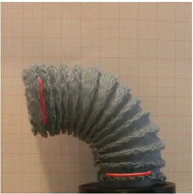
[image:10.595.185.385.341.542.2]

The pneumatic chambers, denoted by the numbers 1, 2, 3, & 4 in figure 1.2a, must be able to elongate individually to create an effective bending of the soft actuator module in a specific direction. A hollow cylinder in the middle of the soft actuator module, denoted by the letter H in figure 1.2a can be used for data cables for e.g. a camera, pneumatic tubes for the next section(s), or other instruments or cables.

Figure 1.1:Soft actuator module bending

The soft actuator module, shown in figure 1.1, is made by 3D printing a mold, which is shown in figure 1.2. This mold is then filled with elastomer to create the actual soft actuator module.

To control the stiffness of the soft actuator module, granular jamming has been implemented by inserting a flexible capsule of very fine coffee powder inside the pneumatic chambers (1, 2, 3, & 4 in figure 1.2a). This capsule has been fixated to the top and bottom, to ensure it gives a uniform stiffness. The way it is activated, is by vacuuming the capsule, which will decrease the volume only slightly but will increase the particle density of the coffee powder resulting in an increased viscosity of the material creating a stiff structure. The granular jamming is part of the actuator, but will not be discussed any further in this report.

(11)

(12)

(13)

(14)

tion as the base frame, an additional multiplication with homogeneous transformation matri-ces with pure rotationRz(φ) andRy(θ) is needed, shown in equation 2.3 and 2.4 respectively.

TRot−_z(φ)=



   

cos(φ) −sin(φ) 0 0 sin(φ) cos(φ) 0 0

0 0 1 0

0 0 0 1

     (2.3)

TRot−_y(θ)=



   

cos(φ) 0 sin(φ) 0

0 1 0 0

−sin(φ) 0 cos(φ) 0

0 0 0 1

     (2.4)

2.2 Robot Specific Mapping

While the robot independent mapping gave a solution for mapping the piecewise constant curvature arc from configuration space to task space, the robot specific mapping will give a solution for mapping the actuator space to the configuration space.

In contrast to the independent mapping, the specific mapping is unique to the exact type of robot. The specific mapping requires measurements on the actual robot, by relating the inputs and outputs of actuators [9]. In case of the soft actuator module the inputs will be the air pressure, related to the pneumatic chamber lengths, resulting in the arc parameters as output.

2.2.1 Parameters

There are three parameters that define the shape and orientation of the soft actuator module. In the section 2.1 it is described how the parameters are defined in the frame convention. The curvature of the soft actuator moduleκ(q), which is related to the angleθwithθ=κs. The angle of the plane containing the arcφ(q) and lastly, the length of the arc`(q), which describes the length of the backbone of the soft actuator module. The centre denoted by H and shown in figure 1.2a. The dependency onqdescribes that all the parameters are dependent on the joint parameters`iwithi∈[1, 2, 3, 4].

2.2.2 Inverse Solution

To go from arc parameters to chamber lengths, which can be related to the applied air pressure, a modified version of the solution by Bryan and Walker (2006) is used. The design in their paper is based on three tendon lengths, but the solution can be applied to pneumatic actuators such as the soft actuator module and modified to a four chamber length case [5].

The solution is based on the angle at which the pneumatic chambers are placed inside the soft actuator. When using three equally spaced tendons, the angle between them is 2/3π, as shown in their result. When using four tendons, or in case of the soft actuator module pneumatic chambers, this angle becomes 1/2π. The angles then become:φ1=φ,φ₂=φ+1/2π,φ₃=φ+π andφ4=φ+3/2π.

To obtain the pneumatic chamber length, the simplified result from Bryan and Walker (2006), shown in equation 2.5, is used as a basis. It describes the length of the tendon based on the

(15)

CHAPTER 2. MODELLING THE SOFT ACTUATOR MODULE 7

main trunk lengths, curvatureκ, rotationφ, distance from the centre of the trunk to the tendon

dand the number of (cable) segmentsn.

`i=2nsin ³κs

2n

´³1

κ−dsin(φi) ´

(2.5)

Equation 2.5 can be modified to work for a pneumatic chamber instead of a tendon. Parameter

dthen becomes the distance from the centre of the trunk to the centre of the pneumatic cham-ber and because pneumatic chamcham-bers are assumed to inhibit a constant continuous curvature, the numbers of cable segments is equal to infinity. Settingn→ ∞_{and substituting the} appro-priate values forφ, the specific mapping for the four pneumatic chamber actuator is shown in equation 2.6.

f−₁

speci f i c=      `1 `2 `3 `4      =     

`(1−κdsin(φ)) `(1−_κ_d_cos(_φ₎₎ `(1+κdsin(φ)) `(1+κdcos(φ))

     (2.6)

Equation 2.6 shows each pneumatic chamber length based on the arc parametersκ,φ,dand`, but to achieve the required length a pneumatic actuation method is used. The relation between the two will be described in the next section.

2.2.3 Chamber Length to Pressure Relation

To relate the air pressure applied to the pneumatic chambers to the length of these pneumatic chambers, the chamber lengths need to be measured at different air pressures. A curve fitting technique is then used to obtain a continuous curve of the chamber length to pressure relation.

Both the actuated and the non-actuated pneumatic chamber lengths are measured. The effects inflicted (upon each other) by both the actuated and the non-actuated pneumatic chamber are used to create a more accurate simulation, and thus a more accurate control system.

2.3 Constraints

A prediction is made that the piecewise constant curvature only holds for a specific range of angles. By adding constraints to the system, it is made sure that the piecewise constant curvature will always hold for any output angle and that desired bending is realizable. The way these constraints are determined is by examining the physical soft actuator module and checking for which angles the piecewise constant curvature holds.

Another constraint is a kinematic constraint. For a single section the device is underactuated, this means it has less number of actuators then it has degrees of freedom (DoF). As a result, it can not follow all paths in the work space. This can be solved by increasing the number of ac-tuators, thus adding more modules till the number of actuators equals the degrees of freedom. In that case, the robot becomes fully actuated.

(16)

3 Constant Curvature Kinematics

Using the modelling of section 2, kinematics of single and multi module cases can be derived.

3.1 Single Module Kinematics

To get the actuator(s) in their desired position and motion, kinematics is needed. First, the forward kinematics for a single module is determined. This way the shape of the soft actuator module and end effector position is determined by setting the angles. Next, using differential kinematics the end effector velocity can be determined by the rate of change of the angles.

3.1.1 Forward Kinematics

Using equation 2.2 the homogeneous transformation matrix can directly be extracted. Given the angleφ, curvatureκand length`the end effector position in Cartesian space can be deter-mined.

Taking equation 2.2 as the transformation matrix T₁0(q), the transformation from 0 to 1 de-pendend onq=[κ φ]T, with 0 being the base and 1 being the end effector of the (first) soft actuator module, denoted byP1. Then, by multiplyingT₁0(q) with the location of the base will give the end effector positionP1, shown in (3.1), if the base of the soft actuator module was placed in the origin,O=[0 0 0]T aiming upwards in the +z-direction.

P1=T₁0(q)·O (3.1)

3.1.2 Forward Differential Kinematics

Differential kinematics relates the velocities of the joints, ˙q=[ ˙φ κ˙]T, in joint space to the end effector velocity in task space, Cartesian space, v=_{[ ˙}_x _y˙ _z˙_]T_{. This relation is given by the} Jacobian of the robot, denoted byJ.

By taking the time derivative of the transformation matrixT, the result can be used to deter-mine the Jacobian.

Similar to the work of Hannan et. al. (2003), the only velocities of interest are those in thex,y, andzdirection. In such a case, if the time derivative of matrix T looks like equation 3.2, then

Jq˙can be constructed by taking specific elements of equation 3.2, shown in equation 3.3 [4].

˙ T =     

α11 α12 α13 α14

α21 α22 α23 α24

α31 α32 α33 α34

α41 α42 α43 α44

     (3.2)

Jq˙=[α₁₄ α₂₄ α₃₄]T (3.3)

Factoring outJ from (3.3) gives the result in equation 3.4.

J= 



β11 β12

β21 β22

β31 β32



 (3.4)

(17)

CHAPTER 3. CONSTANT CURVATURE KINEMATICS 9

With elements:

β11= 1

κ(−sin(φ)+sin(φ) cos(κs)) (3.5)

β21= − 1

κ(cos(φ)−cos(φ) sin(κs)) (3.6)

β31=0 (3.7)

β12= 1

κ2(cos(φ)−cos(φ) sin(κs))+

s

κcos(φ) sin(κs) (3.8)

β22= 1

κ2(sin(φ)−sin(φ) cos(κs))+

s

κsin(φ) sin(κs) (3.9)

β32= 1

κ2sin(κs)+

s

κsin(φ) sin(κs) (3.10)

Using this Jacobian, the end effector velocity can be determined based on the joint velocity, shown in equation 3.11.

v=Jq˙ (3.11)

The Jacobian also serves as a basis for the inverse kinematics problem [5].

3.1.3 Inverse Differential Kinematics

Obtaining the joint angles based on the end effector position is called the inverse kinematics problem. Multiplying equation 3.11 with the inverse Jacobian on both sides is a solution, how-ever, in this case the Jacobian is not square. This is solved by taking the pseudo inverse of the Jacobian. The pseudo inverse Jacobian, denoted byJ+

, is defined as shown in equation 3.12.

J+

=(JTJ)−1JT (3.12)

This way the end effector velocities can be set, and the joint velocities be determined.

˙

q=_J+_v _(3.13)

As a single module system is underactuated, it cannot follow all arbitrary trajectories. The x, y and z coordinates are dependent on each other. A certain x and y in the work space will results in a forced z coordinate. This does not add any benefit over using the less-complex forward kinematics method, and will thus not be tested on the physical soft actuator. However, the method described is the same as for a multi section inverse differential kinematics problem.

The current end-effector frame rotates together withθandφ. As explained in section 2.1 an additional multiplication withRz(φ) andRy(θ) is needed to have the end-effector frame par-rallel to the base frame in thex,y andz-direction. This will then put the velocities in a more intuitive frame. The velocities are then in the same direction as the base frame.

(18)

(19)

11

4 Implementation

The realization of the control system of the soft actuator module has been done in multiple, separate, steps. First, the physical soft actuator module (section 1.2) is tested in order to char-acterize the bending versus chamber length (section 2.2.3). After, the characteristics of the soft actuator module is determined, namely the relation of the elongation of the pneumatic cham-bers and the applied pressure. This relation is then used, together with equation 2.6 to deter-mine the needed pressure to achieve the required bending angle(s). To verify the simulations and the calibration, the above is evaluated on the physical soft actuator module.

4.1 Soft Actuator Module

The soft actuator module has been created as described in chapter 1.2. The mold, shown in figure 1.2a and 1.2b has been 3D printed and assembled. The mold has then been filled with EcoflexTM00-50 Platinum Cure Silicone Rubber Compound by Smooth-On. The material was then vacuumed for 3 minutes to remove any air bubbles present. It was let to cure for 4 hours before taking the mold apart and applying the shielding.

The shielding makes sure the pneumatic chambers do not expand outwards, and the full de-formation is in the elongated direction. The shielding has been made to fit the soft actuator module closely and only allow expansion in the upwards direction.

When referred to a 2D, scenario, chambers 1 and 3, which can be seen in figure 1.2a are connected to a pressure regulator (manual or voltage controlled). Chambers 2 and 4 in a 2D scenario are left unconnected. In this scenario when referred to the actuated chamber or actuated pneumatic chamber is the chamber with the controlled air pressure in it. The passive, or non-actuated, chamber is at vacuum to stay as close to the original 3.0 cm chamber length.

In a 3D scenario, all 4 chambers are connected to pressure regulators. Furthermore, the 2D and 3D scenario use the same algorithm, only with different calibrations. The above steps are first done in a 2D implementation (φ=0), which is followed by a 3D implementation.

4.2 2D Implementation

4.2.1 Calibration

The calibration is performed to establish the relation between the pneumatic chamber length and the applied pressure. The way this has been performed is by placing specific physical markers on the soft actuator module. A series of increasing known pressures are applied into one chamber, and the bending is examined. This bending is captured with a digital camera, and digitally the size of both the actuated pneumatic chamber and the opposite pneumatic chamber (chamber (1) and (3) in figure 1.2a) is determined. The measuring setup can be seen in figure 4.2.

Physical markers have been placed 5 mm above and 2 mm below the pneumatic chamber, this margin has been introduced to avoid puncturing the chamber with the needle markers. Needle markers have been used to avoid measuring errors of the shielding moving independently from the internal soft actuator module. The total distance from the bottom marker to the top marker in rest position (θ=0) equals those two margins plus the chamber length of 30mm, resulting in 37mm.

(20)

(21)

(22)

(23)

(24)

5 Simulations

The purpose of the simulations is to validate the modelling of the soft actuator module of chapter 2 together with the kinematics of chapter 3.

The simulations are done using the same order as described in section 4. First, a 2D scenario is simulated, which is followed with a 3D scenario. After the single module has been simulated in both 2D and 3D, this is expanded into a 3D multi module simulation.

The purpose of these simulations is to verify the kinematics of the robot. It also gives a visual representation of the shape of the module together with it’s chamber lengths. This could help to spot errors before the physical testing stage.

5.1 2D Single Module

The 2D simulations are based on the equations in section 3.1 withφ=0, the physical limi-tations, described in section 4.4, have also been included in this simulation. A 2D Cartesian system is created in which the base of the module has been placed in [0 0]T. The backbone of the module is then plotted according to the homogeneous transformation matrix given in equation 2.2 given a specificθin the range 0 to 1/2π. `is set to 3.00cm, equal to the physical chamber length.φis set to 0, as mentioned above. A continuous curvature has been achieved by plotting 240 points forsin (2.2), from 0.0cm to 3.0cm, with a resolution of 80 dots per cm.

The pneumatic chambers have been visualized in the same manner as the main backbone, but their bases have been placed in [d 0]T and [−d 0]T withd being the distance from the backbone, the centre of the soft actuator module, to the centre of the pneumatic chamber, which equals 0.8cm.

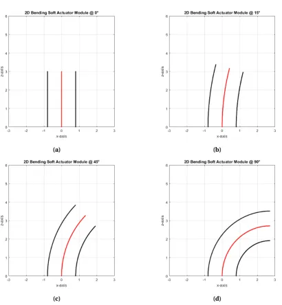
[image:24.595.70.498.595.642.2]

Figure 5.1a - 5.1d show a 2D plot of the main trunk, displayed in red, with the left and right chamber, displayed in black at the angles,θ, of 0◦

, 15◦

, 45◦

and 90◦

, respectively. An angle θ of 0◦

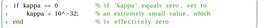
is considered the rest state, however whenθ =_{0 is applied to relation with} _κ=_θ_/_s_, this results in a division by zero in equation 2.2. This has been prevented by adding the code below, which results in the angleθbeing, effectively, 0 while not causing a division by zero. The MATLAB code can be found in appendix A withφ=_0.

1 i f kappa == 0 % i f ’ kappa ’ equals zero , s e t to 2 kappa = 10^−32; % an extremely small value , which

3 end % i s e f f e c t i v e l y zero

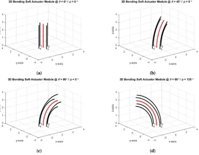
5.2 3D Single Module

The 3D simulations are done in the same fashion as in section 5.1, but in a 3D Cartesian system, and placing the base of the module in [0 0 0]T. The backbone of the module has been plotted as described in section 5.1, with the same resolution,`andθ range. But, in the 3D scenarioφhas been made variable from 0 to 2πinstead of equal, and fixed, to 0.

The four bases of the pneumatic chambers have been placed around the backbone’s base at 90◦

intervals at a distancedof 0.8cm.

(25)

CHAPTER 5. SIMULATIONS 17

(a) (b)

[image:25.595.102.513.71.516.2]

(c) (d)

Figure 5.1:2D simulations of the soft actuator module bending at multiple anglesθ

Figure 5.2a - 5.2d show a 3D plot of the main trunk, displayed in red, with the four pneumatic chambers in the configuration described above. A multiple of configurations are displayed for display-purposes. Similar to section 5.1.1, in case of the rest state, that isθ=0, the same code is used to prevent a division by zero. The MATLAB code can be found in appendix A.

5.3 3D Multi Module

The simulations in section 5.2 serve as a basis for the simulations for a 3D multi module endo-scope. Every module inside the multi module endoscope can be seen as an individual module, such as simulated in section 5.2. The simulations of multi module has been performed in the same 3D Cartesian space as the 3D single module simulations (see section 5.2). The base of the first module has been placed in [0 0 0]T, similar to the 3D single module. But, every suc-ceeding module is placed on the frame of the end effector of the previous module. This can be seen as multiplying the individual homogeneous transformation matrices, shown in equation

(26)

(a) (b)

[image:26.595.87.497.82.402.2]

(c) (d)

Figure 5.2:3D simulations of the soft actuator module bending at multiple angles ofθandφ

3.14. For the simulations for the multi module robot a 2 module case has been created. This way the simulations stay relatively simple compared to a higher number of modules, while still being able to show the possibilities of a multi module robot.

Because the soft actuator module has a non-bending part at the top and bottom, this has also been modelled in the simulations by adding a pure translation transformation matrix in between the homogeneous transformation matrices of the first and second module. This is 0.5cm at the top, and 1.0cm at the bottom.

The pneumatic chamber lengths of each module are also calculated based on the parameters of each individual module. This can be compared with the simulations shown in section 5.2. The individual chambers are not shown in the 3D multi module simulations to avoid clutter.

Figure 5.3a - 5.3d show the simulation results for the multi module robot following the criteria sated above. Multiple configurations are displayed to show the possibilities of this robot. The rotationφi, withi ∈[1, 2], is done at the beginning of each new module. The considered rest state has been displayed in figure 5.3a. The MATLAB code for the 3D simulations can be found in appendix B.

(27)

CHAPTER 5. SIMULATIONS 19

(a) (b)

[image:27.595.97.519.197.555.2]

(c) (d)

Figure 5.3:Multi module simulations showing multiple configurations with the black module being the first one, the blue module the second one and the red pieces are the non-bending parts of the actuators. A line from the origin to the projection of the end effector on thex−yplane can be seen as the thin black

line in thex−yplane.

(28)

6 Results

The results are obtained as described in chapter 4. These are compared to the simulations, the control algorithm, if applicable.

6.1 Validation: Piecewise Constant Curvature Assumption

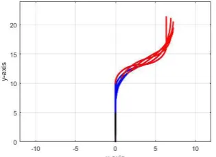
[image:28.595.168.398.249.445.2]

Measurements have been done according to the method described in section 4.2.1. The radius lengthsr1andr2, as shown in figure 4.1, have been measured and the absolute difference be-tween these two is displayed in figure 6.1 for the left and right bending. Figures 6.2 and 6.3 show the soft actuator at multiple angles ofθ.

Figure 6.1:Absolute difference between lengthsr1andr2

Figure 6.2:Left bending at multiple angles ofθ

Figure 6.3:Right bending at multiple angles ofθ

6.2 Chamber Length - Pressure Relation

6.2.1 2D: Calibration

Section 4.2.1 describes the process of obtaining the calibration results and calculations re-quired for it. The results of these measurements and calculations are displayed in figure 6.4 and

(29)

CHAPTER 6. RESULTS 21

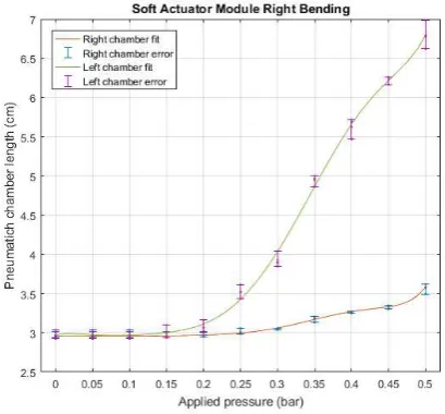
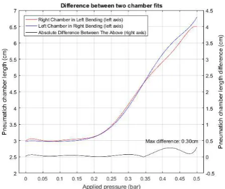
[image:29.595.195.401.160.346.2]

figure 6.5. These figures include the original measuring data, with the maximum and minimum displayed by the errorbar. An 8th degree polynomial has been fitted to the mean value of the measurement data. An 8th degree polynomial is chosen because it would have the least devia-tion from the mean value points. Figure 6.6 shows the fitted curves of both actuated chambers, included the absolute difference between them.

Figure 6.4:2D bending pressure and chamber length relation for a left bending

Figure 6.5:2D bending pressure and chamber length relation for a right bending

With a maximum difference of 0.49 cm at 0.35 bar for the left bending (figure 6.4) and 0.36 cm at 0.50 bar for the right bending (figure 6.5). This difference in chamber length is equal to a 17◦

and 12◦

difference in bending (θ) respectively at that pressure level.

In figure 6.6 the maximum absolute difference of the two curves is 0.30 cm, at that specific pressure (0.50 bar) will result in aθ=10◦bending difference.

[image:29.595.195.400.411.601.2]

(30)

[image:30.595.178.402.84.272.2]

Figure 6.6:Difference of the fit of actuated chambers of figure 6.4 and 6.5

6.2.2 2D: Validation

Following the method described in 4.2.2 the validation of the 2D scenario is executed. The results, the difference of the input bending angle θ (supplied to the control algorithm) and the actual bending, are shown in figure 6.7a for the left bending and figure 6.7b for the right bending of the soft actuator module. Both figures include the error when assuming the passive chamber is at 3.0cm, referred to as “Chamber error without compensation” and the error when compensating the acutated chamber length based on the passive chamber length, referred to as “Chamber error with compensation”.

[image:30.595.79.497.457.653.2]

(a) (b)

Figure 6.7:Difference between the input angle and the measured angle for left and right bending

6.3 3D: Proof of Concept

Figure 6.8 shows a top view of the soft actuator module with a overlay showing the actuated pneumatic chambers, as yellow circles, the passive pneumatic chambers, as blue circles, thex

andy-axis and the direction of bendingφas the yellow line. Figure 6.9 shows the perspective when looking from thex-axis andy-axis in a 3D scenario.

(31)

(32)

7 Discussion

The results of the piecewise constant curvature validation show two different results. One, on the left bending, show that the difference between the radius lengthsr1 and r2 is minimal, proving that the assumption of piecewise constant curvature is valid. However, the right bend-ing shows a larger difference between the two lengths, showbend-ing that the assumption does not hold as well compared to the left bending. When looking at figure 6.3 it can also be observed that compared to figure 6.2 the curvature is less uniform. The soft actuator module elongates more in the right direction and the bending is mostly in the middle, with the top part (referring to the part that is not fixed to the base) containing almost no bending. This is likely caused by the non-uniformity and non-symmetry of the shielding, as it is shrunk by heating it by hand, and thus prone to imperfections. The error does increase with increased bending for both left and right bending, especially the left bending shows an increase in error after 90ci r c. This confirms the prediction made in section 2.3 regarding that the piecewise constant curvature will only hold for a certain range ofθ.

Comparing the calibration results of the left and right bending show similar trend, this can also be seen in figure 6.6 where the fitted curves are compare, however, similar to the validation results, the slight differences can be caused by the non-uniformity and non-symmetry of the shielding as explained above. The validation results of the individual left and right curves show that with the passive chamber compensation the accuracy of the soft actuator module control is greatly increased. It also shows that a larger bending relates to a larger error. The error in the right bending (figure 6.7b) shows a error which deviates from the expected error. A possible explanation for this could be the non-uniformity and non-symmetric construction of the shielding, as explained above in the first paragraph of this chapter.

The use of curve fitting also brings error into the experiments, because the fit is not exact, there is a deviation from the actual measuring results. An increase in accuracy can be achieved by in-creasing the number of measurement points and by experimenting with different curve fittings.

If the physical soft actuator module, including the shielding, could be made uniformly and symmetrically, every pneumatic chamber’s bending could be considered identical requiring only measurements on one pneumatic chamber..

Furthermore, there are multiple causes of uncertainty in the measurements. First, human factor while manually determining the angles and link- and radius lengths in ImageJ. Second, the images taken are slightly distorted due to the camera’s field-of-view, and consequently a non-flat image. Last, the exact location of the internal pneumatic chambers can’t be directly observed. The markers used will also introduce a uncertainty into the measurements.

The repeatability of the calibration measurements can be assessed based on the differences between the multiple measurements. This difference is larger for the left bending compared to the right bending. The error between the minimum and maximum value is considered to be significant, resulting in noticeable angle differences. When concatenating multiple modules the overall error will increase linearly with the number of modules. For this case and the application of the soft actuator module the repeatability is considered to be low.

(33)

CHAPTER 7. DISCUSSION 25

Observation on the prediction made in section 4.3 that the soft actuator needs more pressure to deviate from this natural bending is observed to be the case. With theθ=₉₀◦_{bending with} aφ=45◦ rotation shown in figure 6.9 a pressure of around 0.53 bar was needed. But when bend in a so-called natural direction, explained in section 4.3, the soft actuator module needed around 0.39 bar.

Furthermore, as shown with the 3D proof of concept, with the control of multiple chambers a desired rotation can be achieved. However, more research into the characteristics and cali-bration should be done to correctly control the 3D motion. Once extended into 3D, the single module serves as a solid basis for a multi module with the kinematics described in section 3 or with the application described below.

As an application for this study, based on the forward kinematics and control algorithm of a single module, multiple segment endoscope was guided through a predefined path. Within this study it has been given the name Insertion Dependent Angle Memory Control (IDAMC). IDAMC works as follows, the (human) operator will, with visual feedback from the camera in the tip of the most distal module, control the most distal module of a multi module robot. The operator is able to control the angleθandφ. The operator is also able to insert the endoscope further into the the patient. In this case, the anglesθandφfrom the most distal module will translate to the adjacent module closer based on the insertion. This way the angle stays at a certain location in the human body, making it possible to transverse the endoscope around complex curvatures.

A 2D (φ=0) MATLAB demo, MATLAB code can be found in appendix D, has been made to show the above. It remembers the set angleθin an array based on the insertion parameter

q in cm. It has a resolution of 0.5cm, which can be increased at the costs of a larger memory array. Figure 7.1a - 7.1c shows a three module endoscope that is mounted on a non-acutated base at multiple insertions. If the base of the endoscope is inserted more or less, the angle θis translated over two sections in such a way that the effective angles equal the set angles. Figure 7.1d shows the overlap for the insertionsq =0 toq =10 with a interval of 1. For these simulations a module length of 5 cm is taken and assumed that there is a constant curvature bending throughout the full module length.

Improving on this design is to be able to more accurately follow the set angles. This can be done by decreasing the module length, and to have the same endoscope length increase the number of modules with the same factor.

(34)

(a)Insertion ofq=_{0 cm and}_θ=₉₀◦ _(b)_{Insertion of}_q=_{2 cm. Angle}_θ_{has been}

par-tially translated into the second section (blue module).

(c)Insertion ofq=5 cm (one module length).

Angleθhas been fully translated into the sec-ond section (blue module), and a new angle has been set ofθ= −90◦(red module).

(d)Overlap of the insertionsq=0 cm toq=10

[image:34.595.315.473.413.528.2]

cm with 1 cm intervals

Figure 7.1:2D simulation of path following application with three modules (red, blue and black) and insertion base rod (magenta line)

(35)

27

8 Conclusions and Recommendations

8.1 Conclusions

The main research question in this study was “How to control a soft actuator module for endo-scopic application”. Moreover to controlling the soft actuator, possible applications and future perspectives of the module was also assessed.

The main research question has been successfully answered by creating a control system that is based on changing the pneumatic chamber lengths by applying an air pressure. Required for this is a understanding of the relation between the applied air pressure and the length of the pneumatic chamber. This relation has been experimentally determined, and validated with a maximum error of 9.61◦

and 9.35◦

for the left and right bending respectively. An additional characterization was added to this control system, referred to as passive chamber compensa-tion, and was able to reduce the error to a maximum of 4.74◦

and 4.31◦

respectively.

A proof of concept of 3D motion has been given to show that by actuating multiple modules a effective bending and rotation can be achieved. However, a more complex calibration is needed to use 3D motion in the control system.

With the kinematics of chapter 3 this single module serves as a solid foundation for a multi module solution and can be used as one of multiple identical modules in a multi module robot to allow more complex maneuvers. A possible endoscopic application is given as Insertion Dependent Angle Memory Control (IDAMC). Furthermore, with the use of inverse kinematics given in section 3.2.3, based on the pseudo inverse Jacobian, it is theoretically possible to set an end effector location and obtain the joint angles. This also allows velocity control in thex,y

andzdirection.

8.2 Recommendations

This section is dedicated to give recommendations for future research and aspects of this study what could be improved.

A major improvement for this study would be the production of a uniform and symmetric soft actuator module, mainly the shielding. This could be done by improving the current produc-tion process or developing a new shielding. One could also incorporate a construcproduc-tion in the actually soft actuator that would constrain the sideways expansion, e.g. rigid rings inside soft actuator.

Furthermore, while a better calibration method could be developed. This can be done by improving on the current design using image based calibration with the use of pysical markers or developing a new design based on e.g. lasers or other positional sensing systems. The resolution could also be increased by choosing smaller intervals in the applied air pressure.

In addition, to create the curve based on this calibration different curve fittings could be used. Comparing these curves and experimenting with them could give a better insight in what method would work best.

(36)

Currently the control algorithm is validated using a manual valve. The output pressure, cal-culated by the control algorithm, is applied manually using this valve. The voltage controlled pressure regulator was ordered at the beginning of this study, but was not delivered in time. The control system however is described in section 4.5.

The Insertion Dependent Angle Memory Control could be used together with MR imaging and machine learning to let an algorithm set the angles based on the insertion. This can be done to assist the operator during surgery or suggest paths (e.g. implementing path planning) to the operator.

(37)

29

A Single Module Simulation MATLAB Code

1 % Jorn Jansen

2 % BSc E l e c t r i c a l Engineering 3 % University of Twente

4 % Enschede , the Netherlands 5 %

6 % Single S o f t Actuator Module Simulation Code 7 % Part of EE BSc Thesis

8

9 %% parameters

10 l =3; % length of arc (cm)

11 sk = l ; % length to point on arc (cm) , i f l =s then

endpoint i s taken

12 k = 8 0 ; % r e s o l u t i o n

13 phi = 0*2*pi/360 ; % r o t a t i o n a l about the z a x i s ( degrees ) 14 theta = 103*2*pi/360; % r o t a t i o n about the y a x i s ( degrees ) 15 kappa = theta / sk ; % curvature

16 d = 0 . 8 ; % diameter of the tube

17

18 i f kappa == 0 % s i n g u l a r i t y prevention 19 kappa = 10^−32;

20 end 21

22 r = 1/kappa ; % radius of curve

23

24 %% inverse dependend mapping

25 l 1 = sk *(1−kappa*d*sin( phi ) ) ; % c a l c u l a t i o n of chamber lengths 26 l 2 = sk *(1−kappa*d*cos( phi ) ) ;

27 l 3 = sk *(1+kappa*d*sin( phi ) ) ; 28 l 4 = sk *(1+kappa*d*cos( phi ) ) ; 29

30 Rz = [cos(−phi ) −sin(−phi ) 0 0 ; sin(−phi ) cos(−phi ) 0 0 ; 0 0 1 0 ; 0 0 0 1 ] ; % r o t a t i o n a l matrix to keep the i n d i v i d u a l chambers from r o t a t i n g around the z−a x i s

31

32 %% physical r e s t r i c t i o n s o l v e r ( old method) 33 i f l 1 < 3.000

34 d1 = 3.000−l 1 ;

35 l = l + d1 ; 36 end

37

38 i f l 2 < 3.000 39 d2 = 3.000−l 2 ;

40 l = l + d2 ; 41 end

42

43 i f l 3 < 3.000 44 d3 = 3.000−l 3 ; 45 l = l + d3 ;

(38)

46 end 47

48 i f l 4 < 3.000 49 d4 = 3.000−l 4 ;

50 l = l + d4 ; 51 end

52

53 kappa = theta / l ; 54

55 i f kappa == 0

56 kappa = 10^−32; 57 end

58

59 l 1 = l *(1−kappa*d*sin( phi ) ) ; % r e c a l c u l a t i o n chamber lengths 60 l 2 = l *(1−kappa*d*cos( phi ) ) ;

61 l 3 = l *(1+kappa*d*sin( phi ) ) ; 62 l 4 = l *(1+kappa*d*cos( phi ) ) ; 63

64 %% c a l c u l a t i o n s

65 f i g u r e(’ pos ’, [ 1 0 10 510 3 6 0 ] )

66 f o r s = 0 : 1 / k : l % main backbone plot

67 T1 = [cos( phi ) *cos( kappa* s ) −sin( phi ) cos( phi ) *sin( kappa* s ) (

cos_{( phi ) *(1}−cos( kappa* s ) ) ) /kappa ; sin( phi ) *cos( kappa* s ) cos ( phi ) sin_{( phi ) *}sin_{( kappa* s ) (}sin_{( phi ) *(1}−cos( kappa* s ) ) ) / kappa ; −sin( kappa* s ) 0 cos( kappa* s ) (sin( kappa* s ) ) /kappa ; 0

0 0 1 ] ;

68 V = [ 0 ; 0 ; 0 ; 1 ] ;

69 Q = T1*V ;

70 plot3(Q( 1 ) , Q( 2 ) , Q( 3 ) , ’ r . ’) ; 71 g r i d on ;

72 hold on ; 73 end

74

75 f o r s = 0 : 1 / k : l % pneumatic chamber 1 plot

cos_{( phi ) *(1}−_cos_{( kappa* s ) ) ) /kappa ;} _sin_{( phi ) *}_cos_{( kappa* s )} _cos ( phi ) sin_{( phi ) *}sin_{( kappa* s ) (}sin_{( phi ) *(1}−cos( kappa* s ) ) ) / kappa ; −sin( kappa* s ) 0 cos( kappa* s ) (sin( kappa* s ) ) /kappa ; 0

0 0 1 ] ;

77 V1 = [ 0 ; d ; 0 ; 1 ] ; 78 Q1 = T1*Rz*V1 ;

79 plot3(Q1( 1 ) , Q1( 2 ) , Q1( 3 ) , ’ k . ’) ; 80 hold on ;

81 end 82

cos_{( phi ) *(1}−_cos_{( kappa* s ) ) ) /kappa ;} _sin_{( phi ) *}_cos_{( kappa* s )} _cos ( phi ) sin_{( phi ) *}sin_{( kappa* s ) (}sin_{( phi ) *(1}−cos( kappa* s ) ) ) / kappa ; −sin( kappa* s ) 0 cos( kappa* s ) (sin( kappa* s ) ) /kappa ; 0

0 0 1 ] ;

(39)

APPENDIX A. SINGLE MODULE SIMULATION MATLAB CODE 31

85 V2 = [ d ; 0 ; 0 ; 1 ] ; 86 Q2 = T1*Rz*V2 ;

87 plot3(Q2( 1 ) , Q2( 2 ) , Q2( 3 ) , ’ k . ’) ; 88 hold on ;

89 end 90

cos_{( phi ) *(1}−cos( kappa* s ) ) ) /kappa ; sin( phi ) *cos( kappa* s ) cos ( phi ) sin_{( phi ) *}sin_{( kappa* s ) (}sin_{( phi ) *(1}−cos( kappa* s ) ) ) / kappa ; −_sin_{( kappa* s ) 0} _cos_{( kappa* s ) (}_sin_{( kappa* s ) ) /kappa ; 0}

0 0 1 ] ;

93 V3 = [ 0 ; −d ; 0 ; 1 ] ;

94 Q3 = T1*Rz*V3 ;

95 plot3(Q3( 1 ) , Q3( 2 ) , Q3( 3 ) , ’ k . ’) ; 96 hold on ;

97 end 98

cos_{( phi ) *(1}−cos( kappa* s ) ) ) /kappa ; sin( phi ) *cos( kappa* s ) cos ( phi ) sin_{( phi ) *}sin_{( kappa* s ) (}sin_{( phi ) *(1}−cos( kappa* s ) ) ) / kappa ; −sin( kappa* s ) 0 cos( kappa* s ) (sin( kappa* s ) ) /kappa ; 0

0 0 1 ] ;

101 V4 = [−d ; 0 ; 0 ; 1 ] ;

102 Q4 = T1*Rz*V4 ;

103 plot3(Q4( 1 ) , Q4( 2 ) , Q4( 3 ) , ’ k . ’) ; 104 hold on ;

105 end 106

107 t e x t( 0 , d , 0 ,’ 1 ’) ; % l a b e l chambers 108 t e x t( d , 0 , 0 ,’ 2 ’) ;

109 t e x t(0 ,−d , 0 ,’ 3 ’) ; 110 t e x t(−d , 0 , 0 ,’ 4 ’) ;

111

112 x l a b e l(’ x−a x i s ’) ; % l a b e l a x i s 113 y l a b e l(’ y−a x i s ’) ;

114 z l a b e l(’ z−a x i s ’) ;

115

116 t i t l e( [’ 3D Bending S o f t Actuator Module @ \ theta = ’ num2str( theta

*360/(2*pi) ) ’ \ c i r c / \ phi = ’ num2str( phi *360/(2*pi) ) ’ \ c i r c ’ ] ) ;

117

118 xlim ([−4 4 ] ) ;

119 ylim ([−4 4 ] ) ; 120 zlim ( [ 0 4 ] ) ;

(40)

B Multi Module Simulation MATLAB Code

1 % Jorn Jansen

8

9 %% general parameters

10 k = 2 0 ; % r e s o l u t i o n of plot

11 T = 1 ; % simulation sample time

12

13 %% parameters l i n k 1

14 l 1 = 3 ; % length of arc (cm)

15 sk1 = l 1 ; % length to point on arc (cm) , i f l =s then

endpoint i s taken

16 phi1 = −3/4*pi; % r o t a t i o n a l about the z a x i s ( degrees )

17 theta1 = 1/2*pi; % r o t a t i o n about the y a x i s ( degrees ) (ONLY

POSITIVE ANGLES)

18

19 kappa1 = theta1 / sk1 ; % curvature 20

21 i f kappa1 == 0 % prevent s i n g u l a r i t y 22 kappa1 = 1e−32;

23 end

24 r1 = 1/kappa1 ; % radius of curve

25

26 %% parameters l i n k 2

endpoint i s taken

29 phi2 = 1/2*pi; % r o t a t i o n a l about the z a x i s ( degrees ) 30 theta2 = 1/2*pi; % r o t a t i o n about the y a x i s ( degrees ) 31

32 kappa2 = theta2 / sk2 ; % curvature 33

34 i f kappa2 == 0 % prevent s i n g u l a r i t y 35 kappa2 = 1e−32;

36 end

38

39 %% Non−bending parts modelling between module 1 and 2

40

41 NB1 = [1 0 0 0 ; 0 1 0 0 ; 0 0 1 1 . 5 ; 0 0 0 1 ] ; % matrix Non−

Bending part #1

42 NB2 = [1 0 0 0 ; 0 1 0 0 ; 0 0 1 0 . 5 ; 0 0 0 1 ] ; % matrix Non− Bending part #2

43

(41)

APPENDIX B. MULTI MODULE SIMULATION MATLAB CODE 33

44 %% p l o t s

45 f i g u r e(’ pos ’, [ 1 0 10 510 3 6 0 ] )

46 f o r s = 0 : 1 / k : l 1 % plot f i r s t section

47 T1 = [cos( phi1 ) *cos( kappa1 * s ) −sin( phi1 ) cos( phi1 ) *sin( kappa1 * s ) (cos_{( phi1 ) *(1}−_cos_{( kappa1 * s ) ) ) /kappa1 ;} _sin_{( phi1 ) *}_cos₍ kappa1 * s ) cos( phi1 ) sin_{( phi1 ) *}sin_{( kappa1 * s ) (}sin_{( phi1 ) *(1}−

cos_{( kappa1 * s ) ) ) /kappa1 ;} −sin( kappa1 * s ) 0 cos( kappa1 * s ) (sin ( kappa1 * s ) ) /kappa1 ; 0 0 0 1 ] ;

48 V = [ 0 ; 0 ; 0 ; 1 ] ; % o r i g i n 49

50 i f s == 0

51 Q11 = T1*V ; % begin f i r s t section

52 end

53 i f s == l 1

54 Q12 = T1*V ; % end second section

55 end 56

57 Q1 = T1*V ;

58 plot3(Q1( 1 ) , Q1( 2 ) , Q1( 3 ) , ’ k . ’) ; 59 g r i d on ;

60 hold on ; 61 end

62

63 f o r s2 = 0 : 1 / k : l 2 % plot second section

64 T2 = [cos( phi2 ) *cos( kappa2 * s2 ) −sin( phi2 ) cos( phi2 ) *sin( kappa2 * s2 ) (cos_{( phi2 ) *(1}−cos( kappa2 * s2 ) ) ) /kappa2 ; sin( phi2 ) *cos( kappa2 * s2 ) cos( phi2 ) sin_{( phi2 ) *}sin_{( kappa2 * s2 ) (}sin( phi2 ) *(1−cos( kappa2 * s2 ) ) ) /kappa2 ; −sin( kappa2 * s2 ) 0 cos( kappa2 * s2 ) (sin_{( kappa2 * s2 ) ) /kappa2 ; 0 0 0 1 ] ;}

65

66 i f s2 == 0

67 Q21 = T1*NB1*T2*V ; % begin second section

68 end

69 i f s2 == l 2

70 Q22 = T1*NB1*T2*V ; % end second section

71 end 72

73 Q2 = T1*NB1*T2*V ;

74 plot3(Q2( 1 ) , Q2( 2 ) , Q2( 3 ) , ’b . ’) ; 75 hold on

76 end 77

78 NBF1 = plot3( [ Q12( 1 ) Q21( 1 ) ] , [Q12( 2 ) Q21( 2 ) ] , [Q12( 3 ) Q21( 3 ) ] , ’ r ’

) ; % plot non−bending part #1

79

80 hold on 81

82 Q3 = T1*NB1*T2*NB2*V ; % c a l c u l a t i o n non−bending part #2 83

84 NBF2 = plot3( [ Q22( 1 ) Q3( 1 ) ] , [Q22( 2 ) Q3( 2 ) ] , [Q22( 3 ) Q3( 3 ) ] , ’ r ’) ;

% plot non−_{bending part #2}

(42)

85

86 s e t( [ NBF1 NBF2] ,’ LineWidth ’, 2 ) ; 87

88 hold on ; 89

90 plot3( [ 0 Q3( 1 ) ] , [0 Q3( 2 ) ] , [0 0 ] , ’ k ’) ; % plot "shadow" on x−y plane

91

92 x l a b e l(’ x−a x i s ’) ;

93 y l a b e l(’ y−a x i s ’) ;

94 z l a b e l(’ z−a x i s ’) ; 95

96 xlim ([−8 8 ] ) ;

97 ylim ([−8 8 ] ) ; 98 zlim ( [ 0 8 ] ) ; 99

100 t i t l e( [’ Multi Module bending @ \ theta_1 = ’ num2str( theta1 *360/(2*

pi) ) ’ \ c i r c / \ phi_1 = ’ num2str_{( phi1 *360/(2*}pi) ) ’ \ c i r c / \ theta_2 = ’ num2str_{( theta2 *360/(2*}pi) ) ’ \ c i r c / \ phi_2 = ’ num2str_{( phi2 *360/(2*}pi) ) ’ \ c i r c ’] ) ;

(43)

35

C 2D Control System MATLAB Code

1 % Jorn Jansen

8

9 %% parameters

10 l =3; % length of arc (cm)

11 sk = l ; % length to point on arc (cm) , i f l =s then

endpoint i s taken

12 k = 8 0 ; % r e s o l u t i o n

13 phi = 0*2*pi/360 ; % r o t a t i o n a l about the z a x i s ( degrees ) 14 theta = 90*2*pi/360; % r o t a t i o n about the y a x i s ( degrees ) 15 kappa = theta / sk ; % curvature

16 d = 0 . 8 ; % diameter of the tube

17

18 kappa = kappaconstraint ( kappa ) ; 19

20 r = 1/kappa ; % radius of curve

21

22 mcl = 3 . 0 ; % minimum chamber length

23 Lold = 0 ; % i n i t i a l value Lold

24

25 Rz = [cos(−phi ) −sin(−phi ) 0 0 ; sin(−phi ) cos(−phi ) 0 0 ; 0 0 1 0 ; 0

0 0 1 ] ;

26

28 L = chamberlength ( l , kappa , d , phi ) ; 29

30 %% physical r e s t r i c t i o n s o l v e r 31 done = 0 ;

32 count = 0 ; 33

35 L = chamberlength ( l , kappa , d , phi ) ; 36 l i n i t = chamberconstraint ( L , mcl , l ) ; 37

38 %% physical r e s t r i c t i o n s o l v e r 39

40 while done == 0 % run u n t i l minimum length i s within 1% of the

previous minimum length

41

42 l = chamberconstraint ( L , mcl , l ) ; % c a l c u l a t e backbone length

with compensation

43

44 kappa = theta / l ;

(44)

45

46 kappa = kappaconstraint ( kappa ) ; % check f o r s i n g u l a r i t y 47

48 L = chamberlength ( l , kappa , d , phi ) ; % c a l c u l a t e chamber

lengths

49

50 pa = pressureoutput ( l ) ; % c a l c u l a t e pressure needed 51 mcl = lengthoutputpassive ( pa ) ; % check passive chamber

length

52

53 l = chamberconstraint ( L , mcl , l ) ; % c a l c u l a t e new backbone

length

54

55 kappa = theta / l ; 56

57 kappa = kappaconstraint ( kappa ) ; % check f o r s i n g u l a r i t y 58

59 L = chamberlength ( l , kappa , d , phi ) ; % c a l c u l a t e chamber

lengths again with the new l

60

61 Lnew = max( L ) ; % determine Lnew, t h i s i s the max in a

2D case

62

63 i f ( ( 0 . 9 9 9 9 * Lold<=Lnew) && (Lnew<=1.0001* Lold ) )

64 done = 1 ; % i f within 1% done = 1

65 e l s e

66 done = 0 ; % i f not within 1% done = 0

67 end 68

69 Lold = Lnew ; % Set old value as the new value

70

71 count = count + 1 ; % keep t r a c k of the amount of

i t t e r a t i o n needed

72 end 73

74 PA = pressureoutput (max( L ) ) % output pressure to command window 75

76 %% functions

77 function L = chamberlength ( l , kappa , d , phi ) 78

79 % c a l c u l a t e chamber lengths 80

81 L ( 1 ) = l *(1−kappa*d*sin( phi ) ) ;

82 L ( 2 ) = l *(1−kappa*d*cos( phi ) ) ;

83 L ( 3 ) = l *(1+kappa*d*sin( phi ) ) ; 84 L ( 4 ) = l *(1+kappa*d*cos( phi ) ) ; 85

86 end 87

88 function l = chamberconstraint ( L , mcl , l ) 89

(45)

APPENDIX C. 2D CONTROL SYSTEM MATLAB CODE 37

90 % c a l c u l a t e backbone length 91

92 i f min( L ) < mcl

93 dl = mcl − min( L ) ;

94 l = l + dl ;

95 end 96

97 end 98

99 function kappa = kappaconstraint ( kappa ) 100

101 % check f o r s i n g u l a r i t y 102

103 i f kappa == 0

104 kappa = 10^−32;

105 end 106

107 end 108

109 function ansp = pressureoutput ( l ) 110

111 % pressure output based on chamber length 112

113 PQ = [ 0 . 0 0 0 0.050 0.100 0.150 0.200 0.250 0.300 0.350 0.400

0.450 0 . 5 0 0 ] ;

114

115 ML1 = [ 3 . 0 3 8 3.038 3.038 3.101 3.164 3.517 4.041 5.002 5.717

6.262 6 . 9 8 2 ; PQ ] ;

116 ML2 = [ 2 . 9 2 4 2.924 2.924 2.940 3.009 3.434 3.896 4.866 5.469

6.166 6 . 6 2 3 ; PQ ] ;

117 ML3 = [ 2 . 9 5 1 2.951 2.951 2.998 3.017 3.614 3.847 4.966 5.690

6.257 6 . 7 8 0 ; PQ ] ;

118

119 ML = mean( [ML1( 1 , : ) ; ML2( 1 , : ) ; ML3( 1 , : ) ] , 1 ) ; 120

121 pl = p o l y f i t(PQ,ML( 1 , : ) , 8 ) ; % f i t t e d curve 122

123 syms p ;

124 eqn = ( pl ( 1 ) * (p) ^8) +( pl (2) * (p) ^7) +( pl (3) * (p) ^6) +( pl (4) * (p) ^5) +(

pl ( 5 ) * (p) ^4) +( pl (6) * (p) ^3) +( pl (7) * (p) ^2) +( pl (8) * (p) ) +( pl (9) ) == l ; % inverse of the f i t t e d curve

125 solp = solve ( eqn , p , ’ r e a l ’, true ) ; %pressure output 126 solpa = vpa ( solp ) ;

127 solpadouble = double ( solpa ) ;

128 ansp = solpadouble ( ( solpadouble >= 0 . 2 ) & ( solpadouble <= 0 . 5 ) )

; % get r e a l solution withint the range of 0 . 2 bar to 0 . 5 bar

129 130 end 131

132 function l = lengthoutputpassive ( pa )

(46)

133

134 % c a l c u l a t e passive chamber length based on pressure applied to

the

135 % actuated chamber 136

137 PQ = [ 0 . 0 0 0 0.050 0.100 0.150 0.200 0.250 0.300 0.350 0.400

0.450 0 . 5 0 0 ] ;

138

139 ML1 = [ 3 . 0 7 1 3.071 3.071 3.071 3.071 3.041 3.001 3.075 3.200

3.345 3 . 4 8 7 ; PQ ] ;

140 ML2 = [ 3 . 0 0 7 3.007 3.018 3.021 3.009 2.986 3.055 3.136 3.291

3.339 3 . 5 0 2 ; PQ ] ;

141 ML3 = [ 2 . 9 8 2 3.001 3.001 3.008 2.991 2.984 3.008 3.062 3.170

3.371 3 . 4 6 4 ; PQ ] ;

142

143 ML = mean( [ML1( 1 , : ) ; ML2( 1 , : ) ; ML3( 1 , : ) ] , 1 ) ; 144

145 pl = p o l y f i t(PQ,ML( 1 , : ) , 8 ) ;

146 l = ( pl ( 1 ) * ( pa) ^8) +( pl (2 ) * ( pa) ^7) +( pl (3 ) * ( pa) ^6) +( pl (4 ) * ( pa) ^5)

+( pl ( 5 ) * ( pa) ^4) +( pl (6 ) * ( pa) ^3) +( pl (7 ) * ( pa) ^2) +( pl (8 ) * ( pa) ) +( pl ( 9 ) ) ;

147 148 end

(47)

39

D 2D Insertion Dependent Angle Memory Control

MATLAB Code

1 % Jorn Jansen

8

9 %% general parameters

10 k = 2 0 ; % r e s o l u t i o n

11 d = 1 ; % diameter of the tube to pressure chamber

12

13 %% base section parameters

14 O = [ 0 ; 0 ; 0 ; 1 ] ; % l o cati on base 15 q = 0 ;

16

17 %% section 1 parameters

endpoint i s taken

20 phi1 = 0 ; % r o t a t i o n a l about the z a x i s ( degrees ) 21 theta1 = 0 ; % r o t a t i o n about the y a x i s ( degrees ) 22 kappa1 = theta1 / sk1 ; % curvature

23

24 i f kappa1 == 0 %prevent s i n g u l a r i t y 25 kappa1 = 10^−32;

26 end 27

29

30 l11 = sk1 *(1−kappa1 *d*sin( phi1 ) ) ; % lengths of the pressure

chambers ,

31 l12 = sk1 *(1−kappa1 *d*cos( phi1 ) ) ; % these can be r e l a t e d to the

pressure

32 l13 = sk1 *(1+kappa1*d*sin( phi1 ) ) ; % applied . 33 l14 = sk1 *(1+kappa1*d*cos( phi1 ) ) ;

34

36 l 2 = l 1 ; % length of arc (cm)

endpoint i s taken

41

42 i f kappa2 == 0 %prevent s i n g u l a r i t y

(48)

43 kappa2 = 10^−32;

44 end 45

47

chambers ,

pressure

52

54 l 3 = l 1 ; % length of arc (cm)

endpoint i s taken

59

62 end 63

65

chambers ,

pressure

70

71 %% memory 72 n = 2 ;

73 Q = [ 0 : 1 / n : 5 0 ] ;

74 THETA = [Q; zeros( 1 , 5 0 *n+1) ] ; % create theta array to

s t o r e angles f o r multiple displacements

75

76 THETA( 2 , 10*n+1:15*n) = 1/2*pi/ ( l 1 *n) ; % s e t t e s t angle theta 77 THETA( 2 , 15*n+1:20*n) = −1/2*pi/ ( l 1 *n) ; % s e t t e s t angle theta

78

79 %% v i s u a l i s a t i o n

80 f i g u r e(’ pos ’, [ 1 0 10 510 3 6 0 ] )

81 f o r q = 10:−1:0 % overlap i n s e r t i o n s q = 10 t i l l q = 0 82 theta1 = sum(THETA( 2 , q*n+1:(q+l1 ) *n) ) ;

83 theta2 = sum(THETA( 2 , ( q+ l 1 ) *n+1:(q+l1+l2 ) *n) ) ;

84 theta3 = sum(THETA( 2 , ( q+ l 1 + l 2 ) *n+1:(q+l1+l2+l3 ) *n) ) ; 85

86 kappa1 = theta1 / l 1 ; 87 kappa2 = theta2 / l 2 ;

(49)

APPENDIX D. 2D INSERTION DEPENDENT ANGLE MEMORY CONTROL MATLAB CODE 41

88 kappa3 = theta3 / l 3 ; 89

92 end 93

96 end 97

100 end 101

102 T0 = [1 0 0 0 ; 0 1 0 0 ; 0 0 1 q ; 0 0 0 1 ] ; % base section

v i s u a l i s a t i o n

103 V = T0*O; 104

105 plot( [O( 1 ) V( 1 ) ] , [O( 3 ) V( 3 ) ] , ’m’, ’ LineWidth ’, 2 ) ; % plot base

of endoscope

106

107 g r i d on ; 108 hold on ; 109

110 f o r s1 = 0 : 1 / k : l 1 % v i s u a l i s a t i o n section

1

111 T1 = [cos( phi1 ) *cos( kappa1 * s1 ) −sin( phi1 ) cos( phi1 ) *sin( kappa1 * s1 ) (cos_{( phi1 ) *(1}−cos( kappa1 * s1 ) ) ) /kappa1 ; sin( phi1 ) *cos( kappa1 * s1 ) cos( phi1 ) sin_{( phi1 ) *}sin_{( kappa1 * s1 ) (}sin( phi1 ) *(1−cos( kappa1 * s1 ) ) ) /kappa1 ; −sin( kappa1 * s1 ) 0 cos( kappa1 * s1 ) (sin_{( kappa1 * s1 ) ) /kappa1 ; 0 0 0 1 ] ;}

112 Q1 = T0*T1*O;

113 plot(Q1( 1 ) , Q1( 3 ) , ’ k . ’) ; 114 hold on ;

115 end 116

2

118 T2 = [cos( phi2 ) *cos( kappa2 * s2 ) −sin( phi2 ) cos( phi2 ) *sin( kappa2 *

s2 ) (cos_{( phi2 ) *(1}−cos( kappa2 * s2 ) ) ) /kappa2 ; sin( phi2 ) *cos( kappa2 * s2 ) cos( phi2 ) sin_{( phi2 ) *}sin_{( kappa2 * s2 ) (}sin( phi2 ) *(1−_cos_{( kappa2 * s2 ) ) ) /kappa2 ;} −_sin_{( kappa2 * s2 ) 0} _cos_{( kappa2 *} s2 ) (sin_{( kappa2 * s2 ) ) /kappa2 ; 0 0 0 1 ] ;}

119 Q2 = T0*T1*T2*O;

120 plot(Q2( 1 ) , Q2( 3 ) , ’b . ’) ; 121 hold on ;

122 end 123

3

(50)

125 T3 = [cos( phi3 ) *cos( kappa3 * s3 ) −sin( phi3 ) cos( phi3 ) *sin( kappa3 * s3 ) (cos_{( phi3 ) *(1}−_cos_{( kappa3 * s3 ) ) ) /kappa3 ;} _sin_{( phi3 ) *}_cos₍ kappa3 * s3 ) cos( phi3 ) sin_{( phi3 ) *}sin_{( kappa3 * s3 ) (}sin( phi3 ) *(1−cos( kappa3 * s3 ) ) ) /kappa3 ; −sin( kappa3 * s3 ) 0 cos( kappa3 * s3 ) (sin_{( kappa3 * s3 ) ) /kappa3 ; 0 0 0 1 ] ;}

126 Q3 = T0*T1*T2*T3*O;

127 plot(Q3( 1 ) , Q3( 3 ) , ’ r . ’) ; 128 hold on ;

129 end 130 131

132 x l a b e l(’ x−a x i s ’) ;

133 y l a b e l(’ y−a x i s ’) ;

134

135 xlim ([−12 1 2 ] ) ;

136 ylim ( [ 0 2 4 ] ) ; 137

138 end

(51)

43

Bibliography

[1] H. Abidi, G. Gerboni, M. Brancadoro, J. Fras, A. Diodato, M. Cianchetti, H. Wurdemann, K. Althoefer, and A. Menciassi. Highly dexterous 2-module soft robot for intra-organ navi-gation in minimally invasive surgery.Int J Med Robotics Comput Assist Surg., 14, 2018. [2] K. Althoefer. Antagonistic actuation and stiffness control in soft inflatable robots. Nature

Reviews Materials, 3:76–77, 6 2018.

[3] M. Cianchetti, T. Ranzani, G. Gerboni, I. D. Falco, C. Laschi, and A. Menciassi. Stiff-flop surgical manipulator: mechanical design and experimental characterization of the single module.IEEE/RSJ International Conference on Intelligent Robots and Systems (IROS), pages 3576–3581, 11 2013.

[4] M. W. Hannan and I. D. Walker. Kinematics and the implementation of an elephant's trunk manipulator and other continuum style robots. Journal of Field Robotics, 20(2):45–63, 2 2003.

[5] B. A. Jones and I. D. Walker. Kinematics for multisection continuum robots.IEEE Transac-tions on Robotics, 22(1):43–57, 2 2006.

[6] M. Manti, V. Cacucciolo, and M. Cianchetti. Stiffening in soft robotics: A review of the state of the art.IEEE Robotics Automation Magazine, 23(3):93–106, 9 2016.

[7] N. Simaan, K. Xu, W. Wei, A. Kapoor, P. Kazanzides, R. Taylor, and P. Flint. Design and in-tegration of a telerobotic system for minimally invasive surgery of the throat. The Interna-tional Journal of Robotics Research, 28(9):1134–1153, 2009.

[8] K. K. Smith and W. M. Kier. Trunks, tongues, and tentacles: Moving with skeletons of mus-cle.American Scientist, 77(1):28–35, 1 1989.

[9] R. J. Webster III and B. A. Jones. Design and kinematic modeling of constant curvature continuum robots: A review. The International Journal of Robotics Research, 22(13):1661– 1683, 2010.