Implementation of a power efficient DFT based demodulator for BFSK

(1)

1

Implementation of a power-efficient

DFT based demodulator for BFSK

Giovanni Meciani M.Sc. Thesis December 2018

(2)

(3)

Abstract

In wireless communication, the frequency offset is a problem that hinders the communication. It arises from the discrepancy between the frequencies of the oscillator of the transmitter and the one of the receiver. To solve this problem, oscillators with high frequency stability can be employed, at the expense of higher power requirements. As a consequence, this solution can be problematic in Wireless Sensors Network (WSN), where sensor nodes have limited power resources. Another solution is to correct the frequency offset within the demodulation algorithm, thus making it possible to use less power-hungry oscillators.

This thesis focuses on the hardware implementation of an existing offset tolerant demodu-lation algorithm for BFSK modudemodu-lation. Particular attention was posed in making the demod-ulator as power efficient as possible, given its usage in a WSN. To reach this goal, the two Discrete Fourier Transforms were optimised for zero-padding, which is an operation used in the algorithm. These two modifications allowed to save power when compared with the standard radix-2 FFT.

Fixed-point is the chosen data representation. As the word length of the representation is a critical aspect that affects power consumption, an appropriate size was determined by using a procedure that makes use of MATLAB. The complete demodulator is implemented in VHDL and is used to characterise the system, when an FPGA is used in the synthesis process. Relevant results analysed are bit error ratio (BER) with different levels of noise, power consumption with different clock speeds, and resource usage.

(4)

(5)

List of Acronyms

AA Anti-aliasing

ADC Analog to Digital Converter

ALM Adaptive Logic Module

ASIC Application Specific Integrated Circuit

AWGN Additive White Gaussian Noise

BER Bit Error Ratio

BFSK Binary Frequency Shift Keying

BIBO Bounded Input Bounded Output

CFO Carrier Frequency Offset

DDC Digital Down Converter

DFT Discrete Fourier Transform

DSP Digital Signal Processor

FFT-ZP Fast Fourier Transform Zero Padding

FFT Fast Fourier Transform

FP Fixed-point

FPGA Field Programmable Gate Array

IF Intermediate Frequency

IoT Internet of Things

IP Intellectual Property

LNA Low-Noise Amplifier

LUT Look-Up Table

mSDFT Modulated SDFT

OFDM Orthogonal Frequency-Division Multiplexing

SDFT Sliding DFT

SNR Signal to Noise Ratio

(8)

SS Spread-spectrum

ST-DFT Short-Time Discrete Fourier Transform

UNB Ultra Narrowband

UWB Ultra Wideband

VHDL VHSIC Hardware Description Language

(9)

Chapter 1

Introduction

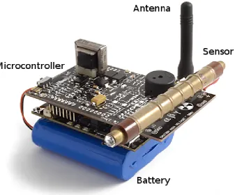
Figure 1.1: Example of sensors. From left to right: thermometer, image sensor, smoke sensor.

The acquisition of information is an important aspect in our lives. We use our five senses to obtain data from our surroundings, but they are neither precise nor reliable. We can tell if the weather today is hot or cold, however we cannot describe it using numbers, which makes the statement consequently subjective.

With the advent of science, which required precise measurements, analog sensors have been invented and improved since the 16th century, when the first thermometer was created by Cornelis Drebbel [1]. Other examples are the barometer to measure pressure, hygrometer for humidity, speedometers for speed, and many other exist to measure different physical variables. Sensors have changed drastically with the coming of integrated circuits. They are now very small, highly precise, and most importantly, can gather information faster than a human could ever read. Imagine if we had to constantly monitor the vital signs of a patient, we would have to spend an excessive amount of time reading the thermometer, the ECG, blood pressure and so on. Thanks to electronic sensors, data can be continuously collected and stored for later use. But what if we have a lot of these sensors, spread over a vast area? We can still place them here and there and check them from time to time. This idea would be feasible, although rather

(10)

Figure 1.2: The dotted signal represents the interference which is wide spread, while the solid line depicts an ultra-narrowband signal.

tedious, when it comes again to patients or to monitor a vineyard or the temperature of each room in your house. However, when safety or security are involved, this option is not viable. In these cases, the information needs to be communicated as fast as possible. As a consequence, sensors have been arranged in what are now called Sensors Network. Each sensor node can communicate its retrieved data to the user, through wires or wirelessly. In the present context, we will focus on the second group which is referred to as Wireless Sensors Network (WSN).

Many WSN are characterised by a very low data rate, in the order of Bytes or kBytes per second. In fact, each sensor reading requires as many bit as the ADC bit resolution in use, which usually spans from a few bit up to 32 bit. Moreover, the transmission of this data occurs every now and then. Sensor nodes rely often on batteries and therefore it is necessary to use the available power as sparingly as possible. Because of that, two approaches have been adopted in order to maintain high power-efficiency in the sensor nodes: duty cycling [2], and wake-up radios [3]. With the first approach, the radio gets ready to receive data at a fraction of the time. This is already an improvement compared to leaving it continuously listening, but it is not optimal. In fact, as it may not be known when the next transmission will occur, the receiver might listen more than it is necessary in order not to miss messages. With the second approach, two radios are employed: a main radio and a wake-up radio. The first one takes care of demodulating the incoming signal and transmit the decoded bits to the microcontroller. Because this operation is power expensive, the wake-up radio, which is designed to be as power efficient as possible, is used to wake the main radio only when it detects a message being transmitted.

Interference is a disturbance produced by the communication between other devices. It is nowadays characterised by wideband signals, for example due to spread spectrum or OFDM techniques. These are usually employed in devices that use Wi-Fi or Bluetooth technologies, such as smartphones, PC, smart appliances, and so on.

In order to avoid it, ultra-wideband (UWB) techniques can be employed. The drawback is the short range that they reach. This is due to the regulations that impose a maximum amount of power that this techniques can use. The Slow Wireless Project proposes to utilise ultra-narrowband (UNB) techniques to realise robust, power-efficient, ad-hoc radio links for WSN that require low instantaneous data rates (Bytes/second). To understand how UNB signals can be useful in wideband interference such as spread spectrum (SS), an example is shown in Fig. 1.2. The dotted signal represents the interference which is characterised by a wideband signal. The solid line indicates an ultra-narrowband signal. Its power is concentrated in a very small bandwidth, while its power spectral density stands decisively above the interference. As a consequence, the signal can be better discriminated by the receiver.

(11)

[image:11.595.131.469.93.373.2]

1.1. WIRELESS SENSOR NETWORK 11

Figure 1.3: Example of a wireless sensor node.

offset tolerant demodulation algorithm for a BFSK modulation technique. Before presenting the algorithm, an overview of WSN is given in the next section.

1.1 Wireless Sensor Network

A Wireless Sensor Network (WSN) is a collection of sensors physically distant to one another that gather information and transmit them in a wireless manner. Usually, physical variables like temperature, humidity, air pressure, etc. is the data being collected. In a WSN there are usually two types of nodes. Sensor nodes obtain the relevant data from the environment and constitute the majority of the nodes. The other type is gateway node, which gathers the information transmitted by the sensor nodes and passes them to the user [5].

A node is usually composed by a radio transceiver, a microcontroller, at least one sensor, and a power supply. An example is shown in Fig. 1.3. The radio transceiver is required to send and receive data, although the latter functionality may not always be present. In fact, a sensor needs to receive data only if it can be controlled. The microcontroller is used to collect data from the sensor(s) and pass them to the transmitter, as well as receiving configuration instructions, for example the frequency at which the data should be transmitted. At least one sensor is connected to the node, although the system might incorporate multiple sensors.

(12)

component [6], modulation and demodulation techniques need to be designed as energy-efficient as possible.

WSN are becoming more adopted in many different fields. In [7], an extensive taxonomy of WSN applications is proposed. WSN can be characterised as single or multi-hop. In the former case, a message sent by a sensor node is directly dispatched to the user node. Instead, in multi-hop, a message is first sent to other nodes before reaching the user. Some of the applications where WSN are being used and belong to the multi-hop group are: metropolitan operation, military, civil engineering, environmental monitoring, logistics, position & animals tracking, transportation, automobile, sensor & robots, reconfigurable WSN, and nanoscopic sensors. Instead, single-hop WSN can find application in: industrial automation, health, mood-based services, entertainment, smart office, sports, building automation, home control.

Another classification for WSN takes into account whether nodes are static or mobile [8]. In the first case, the nodes are placed once and remain in the same position indefinitely, conversely, in the mobile WSN nodes can move around. In our work, only static WSN are taken into consideration.

In [7], WSN applications are grouped by data rate. Thirteen out of eighteen of the considered applications are medium or low bit rate, which means they use less than 115.2 kbps. Because of that, ultra-narrowband (UNB) modulation schemes are becoming more widespread [4]. The advantage resides in the longer range that this technique is able to achieve compared with wide-spectrum signals.

1.2 The frequency offset problem

The frequency offset is a non-ideality that arises from the discrepancy between the frequencies of the oscillator of the transmitter and the one of the receiver. This is due to physical limitations caused by the age of the oscillator, its temperature, mass transfer due to contamination, stress-strain in the resonator, and quartz defects [9]. This imperfection is expressed based on deviation from the nominal value of the frequency indicated by the manufacturer in terms of parts per million (ppm). For example if an oscillator is rated 50 MHz with ±20ppm, then its actual frequency is between 50.001 MHz and 49.999 MHz.

If the oscillators were ideal, the two frequencies used to transmit bit “1” and bit “0” would remain unchanged. In reality, the frequency offset problem might occur. This produces a shift of these two frequencies, which makes the receiver unable to detect the incoming data. The lower the data rate, the higher the frequency stability of the oscillator has to be, being equal the carrier frequency. For example, for frequency offset in the order of 20% of data rate and data rate of 1 kbps, 2.4 GHz for the carrier wave, the frequency stability of the oscillator needs to be less than±1ppm. A crystal oscillator with low frequency stability is not only expensive, but also more power-hungry [4]. However, that is not desirable in sensor nodes powered by batteries.

This problem can be addressed in the digital or analog domain or both. A number of algorithms have been proposed for the digital domain [10–12], but they can only partially solve the problem. Another possible solution is to pass the burden of implementing frequency offset cancellation techniques to demodulation and detection schemes. This, in turn, helps to ease the constraints on the crystal by making it possible to adopt a less precise one, which ultimately makes the system more power-efficient [13].

(13)

1.3. ST-DFT DEMODULATION SCHEME 13

Figure 1.4: Diagram of the proposed demodulator [4].

BPSK the Auto-Correlation Demodulator is employed [16, 17]. The ST-DFT demodulation is the centre of this thesis and will be explained further in the next section.

1.3 ST-DFT demodulation scheme

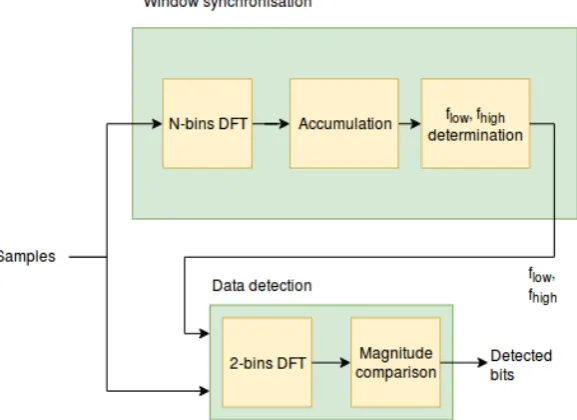
In the previous section it was illustrated how the frequency offset problem may negatively affect the communication. In this section, an algorithm presented for BFSK modulation will be presented which is capable of tolerating large frequency offset by employing the Short-Time DFT [4]. In Fig. 1.4 its block diagram is shown. Initially, samples are acquired. A window is then aligned over a symbol, in the synchronisation phase. These samples are then processed by the ST-DFT block, which produces the power spectral density of the signal. By using this representation, it is possible to determine at which frequencies the transmitter is sending the data. Hence, a frequency offset would not hinder the correct data detection, because the frequencies are determined whenever a new data packet is received. As soon as the synchronisation is complete, the information regarding the detected frequencies is then passed to the detection block, indicated bybLandbH. At this point, the ST-DFT is used to determine

the actual bits contained in the data packet. The algorithm will be explained in more details in Section 2.1.

1.4 Radio receiver

In this section, a radio receiver will be outlined which will give an idea of where the demodulator is placed. A generic schema for a radio receiver is presented in Fig. 1.5. A description of the flow of the signal from the antenna to the demodulator according to the previous figure is as follows.

1. Anantenna is an electronic circuit that produces or captures radio waves. In our case it receives the electromagnetic waves and transform them in a signal.

2. The second element is a bandpass filter, which is used to allow a certain range of frequencies to pass through and reject those outside.

3. Next, the signal passes through a low-noise amplifier (LNA). It amplifies the signal, which is at the present stage very low on power. The characteristic of this type of amplifier is to enhance the useful signal, while adding as little noise as possible.

(14)

[image:14.595.171.427.65.300.2]

Figure 1.5: Schema of a generic radio receiver.

local oscillator, is used to shift the signal from the carrier frequency to an intermediate frequency (IF).

5. Subsequently, alow-pass filteris applied to counter the side effect of the previous oper-ation. The mixer brings the signal to a certain frequency fIF. As a result of the mixing

operation, an additional frequency component located in 2fc−fIF is generated, wherefc

is the carrier frequency. Hence, the low-pass filter is used to remove it.

6. At this point, the signal is still in the analog domain. As the demodulator is digital, an ADC is used to convert the signal to the same domain.

7. Next, a digital down converter (DDC) is employed. Recall that after the mixer, the signal is now located in an intermediate frequency. A DDC is employed to bring the signal in the base band, that is to centre it at the zero frequency. This operation is done to further reduce the frequency, which helps to process the signal at lower speed. This in turn, helps to reduce power consumption.

8. Before reaching the demodulator, the signal passes through a decimation filter. Its purpose is to reduce the sampling rate in order to accommodate slower components of the system. Additionally, it helps reduce the processing power, as less samples imply less memory is needed and a slower clock can be employed.

9. Finally, the digital signal reaches thedemodulator and the relevant information can be extracted.

1.5 Research questions

(15)

1.6. THESIS OUTLINE 15

Another important aspect while designing a system is the determination of an appropriate data representation, which is essential for two reasons. Firstly, an incorrect data representation may produce incorrect results, for example due to overflow as a consequence of too small regis-ters. Secondly, it influences the power consumption as more registers and interconnections are needed.

Finally, the produced implementation of the system will be studied. As a power-efficient demodulator is designed, it is relevant to know its power consumption for the technology used to implement it. Additionally, its performance needs to be analysed in order to determine which ADC frequencies can be supported.

To summarise, the research questions are as follows:

RQ1. How can the two DFTs be implemented in a more power-efficient way?

RQ2. What is the smallest number representation so that the BER is the same as when full precision is used?

RQ3. What is the performance and the resource usage of the proposed implementation?

1.6 Thesis outline

(16)

(17)

Chapter 2

Background

In this chapter, the possibility to use more power-aware solutions for the two DFTs, in the synchronisation and the detection blocks will be investigated. As it will be shown, both cases include a special function that enables additional optimisation compared to the standard radix-r FFT.

In Section 2.1 the adopted demodulation algorithm will be further explained. In Section 2.2, the DFT in the synchronisation block will be analysed. Subsequently, in Section 2.3, a solution for the detection phase will be presented.

For the reminder of this text, the conversion from complex to real operation is as follows. It is assumed that when converting from a complex operation to a real one, a complex addition (CA) results in two real additions (RA), while a complex multiplication (CM) is equivalent to

two real additions and four real multiplications (RM).

Additionally, the following notation is used unless otherwise specified

W_Nkn:=ej2πknN .

[image:17.595.155.444.524.734.2]

2.1 Demodulation algorithm

Figure 2.1: Schema of the demodulator.

(18)

The ST-DFT demodulation scheme is used to achieve a frequency offset tolerant communi-cation. It was originally proposed in [15] and improved in [4]. It can be used for differentially encoded BFSK modulation. The algorithm is composed of two phases, namely window syn-chronisation and data detection. The diagram that shows their interconnections is presented in Fig. 2.1. Before describing the role of the two phases, the ST-DFT and zero-padding will be explained.

2.1.1 ST-DFT and zero-padding

0 0 2 2 4 4 Time 0 6 S(f) 10 6 20 DFT bins 30 8 ₄₀ 50 8 60 10 ₇₀ 10

0 10 20 30 40 50 60 70

DFT bins 1 2 3 4 5 6 7 8 9 10 Time

Figure 2.2: (left) Power spectral density obtained by using the ST-DFT. (right) Same repre-sentation viewed from above.

The ST-DFT is a linear transform that produces a time-frequency representation of a signal [18]. This information is useful for example with BFSK modulation. As data is encoded by varying the frequency of the transmitted signal over time, this frequency shift can be easily seen in the frequency domain. An example is shown in Fig. 2.2.

This operation is used both in the synchronisation and detection phase. In the first one, it is needed to detect the symbols present in the preamble of the transmitted packet. In this case, a full N-point DFT is required. In the detection phase, it serves to detect the bits transmitted. As this information is passed on two specific frequencies, in this case the algorithm needs only two bins of the calculated DFT.

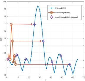
The DFT is performed on zero-padded samples, both in the synchronisation and in the detection blocks. This operation is done to interpolate the bins in the spectrum. To understand the effect of this operation, an example is shown in Fig. 2.3. In this case, the window is composed of eight samples. The non-interpolated line was obtained by computing the 8-point DFT, without applying any zero-padding. The same DFT result is shown with the purple diamonds, but this time the magnitude of the bins have been spaced so that they are eight points apart from each other. Finally, the blue line with full points indicates the interpolated DFT of the same eight samples with a zero-padding factor of 8, which corresponds to a 64-point DFT.

(19)

[image:19.595.149.438.90.364.2]

2.1. DEMODULATION ALGORITHM 19

Figure 2.3: Comparison of different DFT.

different frequencies will fall into the same bin. Instead, thanks to the interpolation produced by the zero-padding, the power spectral density is well spread and the positions of the peaks can be better distinguished. In conclusion, the zero-padding was used to increase the resolution of the incoming signal.

2.1.2 Window synchronisation

The task of the window synchronisation phase is to align the sample window over a symbol. Moreover, this phase detects the bins corresponding to the frequencies used by BFSK, indicated by bL andbH in Fig. 2.1.

To obtain this information, a rectangular window is shifted over the initially arrived samples that belong to the preamble, which is a sequence of alternating zero and one symbols. Each symbol is composed of a fixed number of samples indicated with M. In Fig. 2.4 this shifting procedure is shown for three different delays. When the window exactly aligns with a symbol (delay = 0), its spectrum shows a single clear peak, either on the low frequencyf lowor on the high frequency f high, which are unknown at this stage of the algorithm. When the window is not aligned, multiple peaks are present. Therefore, the idea is to slide the window over the whole preamble and understand which of the M delays is the best one.

(20)

[image:20.595.183.414.83.318.2]

Figure 2.4: Variation of spectrum when the window is delayed [4].

are obtained and stored in register 2. This operation is repeated for M=8 times and involves samples labelled from 0 to 14. This was the first accumulation round, which corresponds to the first symbol. As there are multiple symbols in the preamble, an equal amount of rounds needs to be computed. In the subsequent rounds, the magnitudes are accumulated with the previously computed values. The accumulation is separate for odd and even numbered symbols.

At the end of all the symbols of the preamble, it is determined which register contains the biggest value, which indicates the delay that best alignes with the preamble symbols. Together with this information, the bins that representflow and fhigh are determined (also referred to as

bin low and bin high).

2.1.3 Data detection

The second phase receives timing information necessary to align the window on the incoming data. The ST-DFT produces a time-frequency representation of the incoming signal, so that the detection of the bits can be carried out. An example of this representation is shown in Fig. 2.2. Each axes that starts from the time line indicates a new ST-DFT. The frequency axis shows the bins of the DFT, while the vertical axis is the magnitude of each bin.

The DFT receives M samples, zero-pads them, and computes the result. Compared to the window synchronisation, in this case only two bins of the DFT are required, those indicated by bin low and bin high. The actual detection happens by comparing the magnitudes of the previously computed two bins. Whenever the first is greater than the second, a bit “1” is detected, otherwise it is a “0”.

2.2 DFT in synchronisation block

(21)

2.2. DFT IN SYNCHRONISATION BLOCK 21

Figure 2.5: Shifting of the window when the number of samples per symbol is 8.

Figure 2.6: Window update process.

In the first window (window 1) the system has to wait for the first eight samples before it can start to process them. Subsequently, for window 2, 3, and so on, the oldest sample of the previous window is removed while all the other samples are shifted. This can be seen in window 2, where the second sample is not in the second slot of the window, but it is now in the first one. Then, the newest sample is inserted in the eighth slot. At this point they can be processed and as soon as the 10th _{sample arrives, window 3 can be formed in the same manner.}

The explained procedure is in fact, sliding a window over a series of samples. This encourages us to investigate the possibility to use the sliding DFT.

2.2.1 Sliding DFT

As explained, each window overlaps with the previous one by the M-1 samples that they have in common. This suggests that the DFT bins obtained for the nth window, can be reused for (n+1)th_{window. This is the idea behind the sliding DFT (SDFT) as presented by Jacobsen and}

Lyons in [19]. It is a reinterpretation of the DFT as a filtering operation. This method is useful when the variation of a DFT bin during a time interval needs to be tracked. A conventional DFT necessitates repetition of all computations for each new sample. However, using the sliding DFT, the computation decreases to a simpler “update” operation.

(22)

computa-Figure 2.7: Resonator for a single bin for the original SDFT.

tional cost and numerical stability. In the next section the original work will be presented and will be followed by the modulated SDFT (mSDFT).

Original SDFT The first sliding DFT was proposed in [19] and updated in [20]. Its derivation is now briefly explained. LetSk(n) be the bin computed at time n for frequency index k for an

N-point DFT. With a standard DFT it would be calculated as

Sk(n) = n X

l=n−N+1

x(l)e−j2Nπkl (2.1)

To calculate Sk(n+ 1), the same operation needs to be computed. However,Sk(n+ 1) and

Sk(n) can be related thanks to the circular shift property of the DFT. As mentioned before,

thenth window removes the oldest sample x(n-N) and adds the last arrived, x(n). Additionally, samples that are in common need to be shifted, which is done by multiplying Sk(n−1) by

ej2πkn/N_{. The equation to compute bin k at time n from the previous one at time n-1 is [19]:}

Sk(n) =Sk(n−1)e

j2πk

N −x(n−N) +x(n). (2.2) This formula is correct as long as only the magnitude of the bin is required. A better expression that corrects the phase is given by [20]:

Sk(n) =e

j2πk

N [S_k(n−1)−x(n−N) +x(n)]. (2.3) The cost of this solution can now be derived, with reference to Fig. 2.7. For K frequencies (1≤K ≤N), after L samples (L≥N), when an N-point window is used and assuming complex inputs, the cost is as follows. The total cost is divided into two parts. The cost of sign inversion and first addition (left) and the rest of operations (right). The number of operations for the left part isCL= (L−N)CA, whereCAindicates complex addition. Since the delay register is empty

(23)

for the right part is CR=K((L−1)CA+LCM), whereCM indicates complex multiplication.

The final cost is:

C₍_tot₎=CL+CR=CA(L−N+K(L−1)) +CM(KL).

Note that additional simplifications can be obtained by taking into account the fact that for certain combinations of kand N, the complex factor ej2Nπk becomes a trivial multiplication by 1, -1, j or -j.

In terms of memory, the system requires N+1 registers for a single resonator. If multiple resonators are used (K ≤N), then N+K registers will be needed, as the left part is used for all the resonators.

The stability of this filter is now discussed. The Z-transform of the k-th bin is given by:

H(z) = 1−z

−N

1−ej2Nπknz−1

it has a single pole atz=ej2πknN , which makes the filter marginally stable. In fact, the stability is affected by coefficient precision (number of bits used for representation in hardware), if the precision is not enough the pole moves outside the unit circle which leads to instability. However, if the numeric coefficient is not excessively rounded, the filter is BIBO stable (Bounded Input Bounded Output).

Modulated SDFT (mSDFT) The block diagram of the modulated SDFT is shown in Fig. 2.8 [21].

Figure 2.8: Resonator for a single bin for the mSDFT [21].

This variation of the SDFT takes advantage of the DFT modulation property. Thekthbin is shifted to the position zero. This removes the twiddle factor from the feedback, hence avoiding accumulated errors due to its finite representation. This can be seen by usingk= 0 in Eq. 2.3, it becomesS0(n) =S0(n−1)−x(n−M) +x(n) and the twiddle factor does not influence the computation anymore. In order to produce the desired shift, Eq. 2.3 needs to be multiplied by the factorW_N−km, where m is the phase of the shift. Whenm= 0, the phase of the modulating sequence is 0, when the index increases, also the sequence increases by a factor ofW_N−k. In order to correct the phase, a multiplication byW_Nk(m+1) is required to produceX_nk =W_Nk(m+1)X_n0.

Also for this SDFT, the left side is independent of the bin index and the result can be shared among multiple resonators. This can decrease hardware complexity by reusing the same component. The number of operations can be calculated similarly to the original SDFT. The cost is calculated for K frequencies (1≤K≤N), L samples (L≥N), when a N-point DFT is used and assuming complex inputs. For the left part the cost isCL=LCA. For the right part

(24)

Figure 2.9: Block diagram of the original DFT when zero-padding is taken into account.

C(tot)=CL+CR=K(3L−2)CM +L(K+ 1)CA. (2.4)

In terms of memory, if K resonators are used, then N+2K registers are needed.

2.2.2 Sliding DFT in presence of zero-padding

The SDFT methods can be used to update previously computed bins whenever a new sample arrives. The last sample of the previous window is removed, all the old samples are shifted, and the new one is introduced. This operation though does not take into account the zero-padding operation. Such an operation, as it was illustrated in 2.2, is necessary in the present case and therefore has to be incorporated.

Currently, none of the existing SDFT methods can be utilised in the algorithm. In fact, the zero-padding makes the concept of sliding a window incorrect. This problem can be resolved by using the result proposed in [22]. The authors suggest that since the zero padding only adds zeroes, part of the computation of a single bin can be avoided.

The idea behind this optimisation is as follows. Let N =Z+S be the number of point of the DFT, Z the number of zeros and S the number of non-zero samples. Then a generic bin is calculated, in the standard DFT, as:

X(k) =

N−1

X

n=0

x[n]e−j2πknN (2.5)

the summation can be divided in two parts, because of the tailing zeros:

X(k) =

S−1

X

n=0

x[n]e−j2πknN +

N−1

X

n=S

x[n]e−j2Nπkn

In the second term all values are zeroes and therefore, only the first term needs to be considered.

(25)

[image:25.595.199.390.73.153.2]

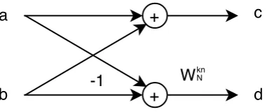
2.2. DFT IN SYNCHRONISATION BLOCK 25 a b + + c d Wkn N -1

Figure 2.10: Butterfly.

with the sliding property. The derivation is as follows.

Xk= N−1

X

n=0

x(n)e−j2πnkN

=

M−1

X

n=0

x(n)e−j2πnkN

=

M−1

X

n=0

x(n)e−j2πnk

0

M

(2.6)

Where N indicates the DFT points, M the number of non-zero samples (N M), k0 = kM N .

The first equality is the N-point DFT. The second equality is obtained by noting that N −M

samples are zero because of the zero-padding. The third equality is a rearrangement of the indices.

The original SDFT can now be revisited in light of this new achievement by starting with Eq. 2.3.

Xk(n) =Xk(n−1)ej

2πk0

M −x(n−M)ej 2πk0

M +x(n)e−j

2π(M−1)k0 M

= (Xk(n−1)−x(n−M) +x(n)WM k 0 M )W

−k0 M

(2.7)

The block diagram of the modified SDFT is shown in Fig. 2.9, withk0= kM

N . The trade-off

here is that while the number of total operations is reduced, a correcting factor appears, which increases the complexity. Moreover, the new multiplication introduces the k factor on the left side, meaning that the computation of this first stage cannot be shared among all the resonators. Only the M registers and the sign inversion operation can be shared.

The cost of the revisited SDFT is as follows. On the left side the cost isCL= (L−M)CA+

KLCM, while on the right sideCR=K((L−1)CA+LCM). The total is as follows.

Ctot =CL+CR= (2KL)CM + (L−M +K(L−1))CA (2.8)

where M is the number of non-zero samples and N the order of the DFT, L is the number of total samples passed to the resonators, and K the number of frequency of interest.

2.2.3 FFT zero padding (FFT-ZP)

The second approach that was studied started by considering the standard FFT radix-2. The reason for choosing radix-2 instead of radix-4 or radix-8 is related to its simplicity. As the order increases, also the structure of each solution becomes more complex.

(26)

[image:26.595.144.449.74.312.2]

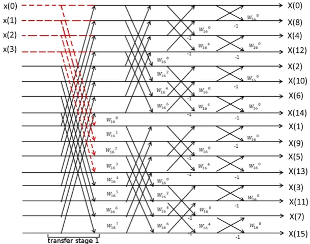
Figure 2.11: 16-points FFT radix-2 DIF.

In the standard radix-2 N-point FFT, there are l stages, where l= log₂N. An FFT stage is a collection of butterflies. An example is depicted in Fig. 2.11. The FFT in the picture is 16-point and the number of stages is 4. The structure of a butterfly is illustrated in 2.10. The interpretation of its flowgraph is as follows; its meaning extends as well to the previously shown FFT stage. The resulting values are c=a+b and d= (a−b)W_Nkn. Usually the plus signs are omitted and the intersection of an arrow into another indicates that a sum is occurring. Instead a factor, like W_Nkn of the example, which lies above an arrow, indicates that it is multiplying the value carried by the arrow.

When M non-zero samples are given to an N-point FFT, with M = 2k _and _N _{= 2}l _and

M < N, then there existl−ktransfer stages andknormal stages. A transfer stage is a stage in which there are no butterflies, cfr. Figs. 2.11-2.13. Because of the presence of the input zeros, in the first l−k stages there are no additions, as they result in passing through the samples. In this case though, the twiddle factors need to be multiplied with the non-zero samples. After

l−kstages, the following stage is a normal one because all its input are at this point non-zero. The cost of this solution is calculated considering that all operations are complex. There are additions only in the last k stages and for each one there are N additions. Considering M = 2k

and N = 2l_{, the number of multiplications can be calculated. There are M multiplications in}

the first transfer stage, 2M in the second one, 4M in the third, and so on. The total number of transfer stages is l-k. Thus, there areMPl−k−1

n=0 2n multiplications in all the transfer stages. In the normal stages there are twiddle factor multiplications which account for N₂ multiplications for each of the last k stages.

Overall, the total number of additions and multiplications are:

CA=kN. (2.9)

CM =M l−k−1

X

n=0

2n+N

(27)

[image:27.595.143.448.108.348.2]

Figure 2.12: 16-points FFT radix-2 DIF. First stage transfers.

[image:27.595.144.450.454.704.2]

(28)

2.2.4 Comparison

In Table 2.1 all the analysed methods for the synchronisation block are summarised. Note that none of the methods take into account the operation reduction due to trivial multiplications by the factors 1, -1, j, -j generated by twiddle factor simplifications.

In general, multiplications are regarded as more power intensive operations than addi-tions. A number of algorithms have been implemented to reduce the complexity of both operations. For the addition, many adders have a logarithmic time. Namely, an n bit in-put Kogge-Stone parallel prefix graph has a delay of log₂n as well as Ladner-Fischer, while Brent-Kung adder has 2 log₂k−2 [23–25]. For the multiplication, the fastest algorithms reach a computational time proportional tonlogn. Mixed-level Toom-Cook implemented by D. Knuth reaches O(nlogn2

√

2 logn_{), the Sch¨}_{onhage–Strassen algorithm improves to} _O₍_n_log_n_{log log}_n_),

and F¨urer’s algorithm takes O(nlogn22 log∗n_{) [26–28].}

These two operations can be compared only when their implementation has been decided. Until that time, they need to be regarded as two incomparable costs. As a consequence, the cost of the DFTs cannot be expressed with a single number and therefore cannot be established unambiguously which one has a lower complexity.

Additionally, the complexity itself also depends, other than on the algorithm, on the tech-nology used (7 nm, 10 nm, 14 nm and so on) and the target IC (FPGA, ASIC, CPU, GPU), among others. It is left to the designer to pick the best combinations depending on the cir-cumstances. In this work, the actual implementation of adders and multipliers was left to the synthesis tool.

The decision of which of these DFTs best suit the present context is postponed to Section 3.1.1, when the parameters of the system will be known, i.e. variables N, M, L, J, etc.

CM CA Note

Radix-2 N

2lJ N lJ [29]

Radix-4 3₈N lJ 3₂N lJ [29]

Split-radix N₄(l−1)J N lJ [30]

SDFT KL L−N +K(L−1) 2.2.1

SDFT revisited 2KL L−M+K(L−1) 2.2.2

mSDFT K(3L+ 1) L(K+ 1−N) 2.2.1

FFT-ZP J(MPl−k−1

n=0 2n+N2k) J N k 2.2.3

Table 2.1: Comparison of the DFT calculation methods studied that could potentially be used in the implementation. N is the DFT order and M is the number of non-zero samples, with

M = 2k_and _N _{= 2}l_{. For the SDFTs, L is the total number of samples present in the preamble,}

for which the sliding operation is necessary; K is the number of bins (it may be less or equal to N). For the standard DFTs, J is the number of times the DFT needs to be repeated to complete the preamble.

2.3 DFT in data detection block

The DFT is also used in the data detection block. In this case it is used to identify whether the received symbol is 0 or 1. The decision is made by comparing the magnitude of the two bins determined in the synchronisation phase. M non-zero samples are zero-padded and sent to a DFT block. However, in this case only two bins are of interest, bin low and bin high. In this section, different methods that optimise the computation based on these conditions are compared.

(29)

2.3. DFT IN DATA DETECTION BLOCK 29

Figure 2.14: Schema of the Goertzel algorithm.

2.3.1 Single bin DFT

A single bin of an N-point DFT can be calculated using Eq. 2.5. It involves N complex multiplications and N-1 complex additions. Therefore, the computation cost in terms of real operations is 4N RM + (4N −2)RA.

In Section 2.2.2, it was shown that the single bin DFT can be improved in presence of zero-padding. In this case the cost becomes equal to M complex multiplications and M-1 complex additions.

2.3.2 Goertzel algorithm

The Goertzel algorithm was firstly presented in [31]; its derivation can also be found in [32]. With this technique it is possible to obtain individual terms of an N-point DFT. The advantage is the reduced amount of operations. This is true as long as the number of bins of interest is equal or less than log₂N, otherwise the FFT outperforms this solution [32]. Only two bins out of the 64 produced by the DFT were required in the data detection, and because of that the previous condition is satisfied. Its schema is shown in Fig. 2.14. The algorithm is a two-stage filter. The first one is:

s[n] =x[n] + 2 cosω0s[n−1]−s[n−2],

which produces an intermediate result. In the second one, the output of the previous stage is used to compute the final value:

y[n] =s[n]−e−jω0_s_[_n₋_1]_, where ω0 = 2_Nπk and s[n] is the output of the first stage.

(30)

and a complex multiplication. The total cost is as follows

Ctot=N(4RA+ 2RM) +CA+CM = (4N + 4)RA+ (2N + 4)RM. (2.11)

The Goertzel algorithm was improved by using the technique described in 2.2.2. The deriva-tion is as follows. The starting point is the same as for the SDFT Eq. 2.6, with k0 = kM/N

and WM =e−j

2π M.

Xk= M−1

X

n=0

x(n)e−j2πnk

0

M

=

M−1

X

n=0

x[n]W_Mnk0

=W_M−k0N

M−1

X

n=0

x[n]W_Mnk0

=W_M−k0(N−M)

M−1

X

n=0

x[n]W_M−k0(M−n)

(2.12)

We define

yk[m] :=

+∞ X

n=−∞

x[n]W_M−k0(m−n)u[m−n] (2.13)

By combining Eq. 2.12 and 2.13

Xk=W

−k0(N−M)

M yk[m]|m=M (2.14)

Notice that

W_M−k0(N−M)=ej2Mπ M

Nk(N−M)

=e−j2πMN k

(2.15)

Finally, from Eq. 2.14

Xk:=e−j

2πM k

N y_k[m]|_m₌_M (2.16)

In Eq. 2.16, it can be seen that the new multiplication factor appears just before the output. This operation can be avoided as it only affects the phase of the result and not the magnitude, which is the only information needed by the algorithm. Therefore, such operation is not included in the cost of the algorithm. Previously, the loop repeated N times, while now only M iterations are needed.

(31)

2.3. DFT IN DATA DETECTION BLOCK 31

2.3.3 Comparison

In Table 2.2, a summary of the previously presented DFT is shown. In this case the operations are all real. This conversion was necessary because the Goertzel algorithm contains a real multiplication, which cannot be converted in term of complex operations.

For both the single bin DFT and the Goertzel algorithm, the improvement produced by the optimisation indicated in 2.2.2, makes the cost become linear in the number of non-zero input values (M) rather than the number of points of the DFT (N).

The decision of which of these DFTs best suit the present context is postponed to Section 3.1.2, when the parameters of the system will be known, i.e. variables N, M, L, J, etc.

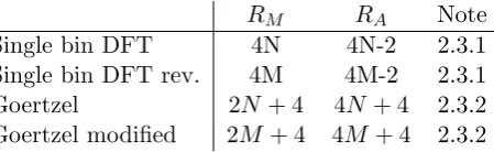
RM RA Note

Single bin DFT 4N 4N-2 2.3.1

[image:31.595.189.414.212.281.2]

Single bin DFT rev. 4M 4M-2 2.3.1 Goertzel 2N+ 4 4N+ 4 2.3.2 Goertzel modified 2M + 4 4M + 4 2.3.2

(32)

(33)

Chapter 3

Design, implementation, and

verification

In this chapter, the proposed implementation of the demodulation algorithm described in Section 2.1 is presented. This chapter opens by presenting implementation considerations regarding the choice of the two DFTs 3.1. Following, the data representation will be discussed 3.2. Next, the system architecture is explained by elaborating on the design blocks that compose the demodulator 3.3. The chapter closes with a presentation of the tools used to verify the design and the methodology adopted for the verification 3.4.

3.1 Implementation

3.1.1 DFT in the synchronisation block

In Section 2.2, different alternatives for the DFT in the synchronisation block were considered. In the present section, their computational complexity will be revisited with defined parameters of the system. The number of samples per symbol, indicated with M, is 8, which is also the size of the window that is used in the SDFT and corresponds to the number of non-zero samples. The number of DFT points, indicated with N, is 64, while the number of times a DFT has to be repeated for a complete preamble, indicated with J, is 112. For the SDFTs, two additional parameters were defined. The number of samples in the preamble, indicated with L, is equal to 119, while the number of bins that need to be computed, indicated with K, is equal to 64.

Table 3.1: Comparison of the DFT calculation methods defined in Table 2.1 when evaluating for afull preamble. N=64, M=8, J=112, K=64, L=119, l=6, k=3. Input is a complex sequence, all the operations are real.

RM RA Note

Radix-2 86,016 129,024 [29] Radix-4 64,512 161,280 [29] Split-radix 35,840 103,936 [30] FFT-ZP 68,096 77,056 2.2.3 SDFT revisited 60,928 45,790 2.2.2

In Table 3.1 each implementation is reevaluated when considering the aforementioned pa-rameters. Split-radix has the lowest number of real multiplications, while the revisited SDFT has the lowest count of real additions. From this table it is evident that the Split-radix and the SDFT are the best candidates to be implemented in the synchronisation block. To choose the best one, the complexity of their structures are now considered. The Split-radix is a combina-tion of FFT radix-2 and radix-4 [33]. Instead, the SDFT has a straightforward structure which

(34)

comprises of only four operations, which is easier to implement. At this point, the SDFT is the best candidate to be implemented.

Before making a final decision, there is another aspect to be considered. In all the DFTs, there are twiddle factors that equal to 1, -1, j, or -j. These values can be efficiently computed by treating them as special cases. In Table 3.2 a summary is presented of the number of real operations required to compute a full preamble, when simplifications are taken into account. The FFT-ZP is the solution that best takes advantage of this simplification, while the SDFT results to be the worst. While the SDFT has the lowest count of additions, it has the worst count of multiplications, which is almost three times the number used by the split-radix or two times the FFT-ZP. Because of this, the SDFT was discarded. The split-radix and the FFT-ZP are the last two candidates. The second has one-third more multiplications than the split radix, but less than half of the additions of the split-radix. In numbers, the price to save 50k additions is roughly 6k multiplications. As it was explained before, comparing these two numbers is not possible until additional information is provided regarding the implementation of these operations. Therefore, their structures will be compared to make a final decision. The split-radix is a combination of radix-2 and radix-4, while the FFT-ZP is a simplified radix-2. In conclusion, the FFT-ZP was deemed the best compromise in terms of ease of implementation and computational cost.

Table 3.2: Comparison of the DFT calculation methods when evaluating for afull preamble. N=64, M=8, J=112, K=64, L=119, l=6, k=3. Input is a complex sequence, operations are realand trivial multiplications are removed.

RM RA Note

Radix-2 29,568 115,584 [33] Radix-4 23,296 109,312 [33] Split-radix 21,952 107,968 [33] FFT-ZP 27,328 56,672 2.2.3 SDFT revisited 57,120 45,790 2.2.2

3.1.2 DFT in data detection block

In Table 2.2, different methods to compute a single-bin DFT were presented. Similarly to what was done for the synchronisation block, these methods will now be revisited in light of the defined parameters. The number of samples per symbol, indicated with M, is 8, while the number of DFT point, indicated with N, is 64.

In Table 3.3 the cost for calculating a single bin DFT is reported in terms of real opera-tions for each methods. The revisited Goertzel algorithm has 12 multiplicaopera-tions less than the revisited single bin DFT, while this second one has 6 less additions. Since multiplications are computationally more intensive than additions, the Goertzel algorithm was considered as the best solution between the two.

Table 3.3: Number of real operations for the data detection, for a single bin and a 64-point DFT, where only the first 8 samples are non-zero.

RM RA Note

Single bin DFT 256 254 2.3.1 Single bin DFT rev. 32 30 2.3.1

Goertzel 132 260 2.3.2

(35)

3.2. DATA REPRESENTATION 35

3.2 Data representation

3.2.1 Fixed-point representation

A fixed-point representation was chosen above floating-point. The latter has a lower power efficiency, which is due to the additional hardware required to carry out operations like addition and multiplication [34, 35]. Moreover, the dynamic range of the input data of the system was limited between -100 and 100. This is in contrast with the practice of using floating-point, which is more suitable when data with different order of magnitudes are present [34].

The fixed-point number representation is a data type used to represent real values. Its advantage resides in the hardware. Operations like addition, multiplication, square root algo-rithms and any other mathematical operation that can been used for integer arithmetic can also be used for fixed-point values. This is the case because fixed-point representation is equal to integer representation, except that the first is scaled by a predetermined factor. This factor though, does not affect the actual computation, but is only used to interpret the results. An example to clarify this concept will be presented later.

Similar to integers, fixed-point numbers can be signed or unsigned. Besides, signed values can be achieved either with two’s complement or signed magnitude. Consider an unsigned N-bit integer value, its binary representation is given by

x=

N−1

X

i=0

bi2i, (3.1)

wherebiis theithbit. Each bit has a weight given by its position, i.e. bitith has weight 2i. The

weights in this case are only powers of two, between 1 and 2N−1_{. With fixed-point, also negative} powers of two are used, which make it possible to represent real values. For the remainder of this thesis, (i|f) denotes a fixed-point number in which iindicates the number of bits used for the integer part andf for the fractional part. For example, given an unsigned number represented in binary as (10010110)2 and FP representation (5|3), then the bit weights are between 2−3 and 24_{, which gives the value} P5−1

i=−3bi2i = 18.75. Another way to obtain the same result is by interpreting the binary representation as an integer in base 10, (10010110)2 = (150)10, and then multiplying it by the weight of the LSB, which is in this case 2−3_{. As expected, the result} is the same 150∗2−3_{= 18}_._75.

When operating with two values that use different FP representations, the user needs to keep in mind the representations in order to interpret correctly the result. For example, let

a have FP (ia|fa) and b have FP (ib|fb). When adding these two values, the one with the

smallest fractional part needs to be adapted to the other. Assumingfa > fb, then the addition

is obtained asa+b∗2fa−fb_{. In this case the FP representation of the result is given by}_a_because of the bigger fractional part.

The multiplication is instead easier. Let cbe the result of a∗b, then its FP representation is (ia+ib|fa+fb). In this case the multiplication can be immediately carried out in integer

arithmetic and later the result can be interpreted as a real value by dividing it by 2fa+fb_. This shows that, except for a shifting operation in the addition, the two operations are the same both in integer arithmetic and in fixed-point. Therefore, the hardware to compute the result can be the same. Similar reasoning applies for division and square root.

3.2.2 Fixed-point optimisation

(36)

[image:36.595.76.523.77.375.2]

Figure 3.1: Block diagram of the demodulator.

processing unit need to be driven in order to obtain the result, which in turn leads to higher power consumption. Interconnections are not only present inside an arithmetic unit, but they serve to move data between different blocks. Each wire acts as a capacitor which drains energy when charged and discharged. As such, the total energy consumption is proportional to the number of interconnections, which is dependent on the data word length.

Registers are needed where intermediate results need to be stored. These elements retain information across subsequent clock cycles. It is in fact the system clock that dictates the frequency at which the content can change. Whether the content of a register changes or not, they still consume energy. Therefore, the higher the number of registers in use, the higher the energy consumption. However, the size of a register is strictly related to the data representation, hence another reason for keeping the word length as small as possible.

The third aspect is the precision of the computation. In the present algorithm there are many values that depend on the sine and cosine functions. The more precise the results need to be, the more the number of digits have to be stored. This translates to larger word lengths, with all the consequences described earlier. Therefore, it is important to maintain the precision just high enough to obtain correct results.

In conclusion, motivated by these three reasons, the next section will present the approach adopted to determine the FP representation. The procedure will strive to obtain word length as small as possible, while ensuring correct results.

3.2.3 Determination of the optimal fixed-point representation

(37)

transmitted bits with those actually decoded. The system was tested for 14 different levels of noise,Eb/N0 = 1,2, ..14dB, withinfinite data precision, that is by using the MATLAB default data type which is 64 bit floating-point. The resulting curve was then used as the performance measure for fixed-point optimisation, which will be referred from now on as the reference curve.

Optimal fixed-point representation of a certain entity of the system means the (i|f) combi-nation that is as small as possible, while the results are still correct. To determine whether the results were correct or not, the BER curve generated by each FP representation was compared against the reference.

The entities for which the FP representation was determined, are shown in Fig. 3.1 with red borders (also for the ADC, which is not depicted). The determination was carried out as follows. The input and output values of the studied block were recorded while running the MATLAB script. The biggest absolute values were used to have a first, rough estimation of the required word lengths. Next, a formal reasoning was adopted to determine the correct representation necessary to avoid overflow. For example, squaring an n bit value requires 2n bit for the output; adding two n bit values require n+1 bit for the output, and so on. Gathering these information, input, output, and formal values, was vital because the number of suitable FP representations is infinite. Instead, with this approach a general idea of where to start searching for the best (i|f) combination was obtained.

As the MATLAB data are in floating-point, a conversion function to fixed-point was needed. The conversion function is as follows.

1 v a l u e = s i g n( v a l u e )∗mod(f l o o r(a b s( v a l u e )∗2ˆ f ) , 2ˆw) /2ˆ f ; 2

where f is the number of bits for the fractional part, w the word length, and value is the data that is being converted. This conversion function can be applied after every basic operation (addition, multiplication, square root). For example, if the following equation needs to be evaluated f(x) = 2x2₋₃_x_{+ 7, the FP conversion function can be placed at different} stages of the computation: on the input, on the output, after computing 2x2, or after 2x and then again after −3x+ 7, after each multiplication, or any other combination. The trade off is between a very close representation, when a lot of conversions are executed, and a fast execution time of the script, when a few conversions are used.

The determination of the FP representation was done for each block separately. Initially, all blocks were set to use infinite precision. When a representation was obtained for a block, the following one were simulated while maintaining the FP of the previous equal to the one just determined, while the subsequent were still left with infinite precision. To clarify, an example is now presented. With reference to Fig. 3.1, let us take into consideration only FFT-ZP, bank of magnitudes (BOM), and bank of adders (BOA). Initially all three are given FP +∞. Then the FFT-ZP FP is determined. At this point, BOM and BOA still have +∞, while FFT-ZP has FP (a|b). In the next step, the FP for BOM is determined while maintaining (a|b) for FFT-ZP and +∞for BOA. After the determination, BOM has a defined FP (c|d) and the procedure can finally be repeated once more for the BOA block.

This sequential determination was done for the synchronisation and detection block sepa-rately. All the FP were then put all together in (Section 3.2.12). In this final step, only some adjustments on the various FP representations were needed in order to obtain an acceptable BER.

(38)

0 2 4 6 8 10 12 14

E_b/N₀ [dB]

10-6 10-5 10-4 10-3 10-2 10-1 100

BER

[image:38.595.156.428.86.335.2]

reference 2 bit 3 bit 4 bit 5 bit 6 bit 7 bit 8 bit

Figure 3.2: Comparison of different ADC resolutions.

3.2.4 Modelling the ADC

The precision of the digital input to the demodulator is determined by the ADC. It was necessary to model it in order to determine the minimum number of bits necessary to represent the input values, while maintaining the BER as close as possible to the reference. As the input was complex, it was assumed that two ADCs were present, for the real and imaginary parts. Similarly to fixed-point optimisation, the model of the ADC was tested in the MATLAB script. The ADC used uniform quantisation with mid-riser characteristic. The values exceeding the threshold were clipped. The threshold, or saturation level, varied dynamically and was set equal to the square of the RMS of the incoming signal.

The results are shown in Fig. 3.2. For bit resolutions between 2 and 4, the distance from the reference curve is noticeable. Instead, for 5 and 6 the difference is relevant only by zooming in at the highestEb/N0 levels, nonetheless it is still relevant. Finally, the curves 7 and 8 bit are both very close to the reference. The latter was chosen as a conservative decision.

This part of the design was carried out for the sake of completeness. Additional research should be performed in order to determine whether a lower amount of bit could have been used.

3.2.5 FP data representation - ADC

Data produced by the ADC are integer values. Generally speaking, all the data processed by the hardware are integers. This is the case because, as it was explained earlier, fixed-point and integer values are two faces of the same coin. Their difference is a scaling factor used to interpret them.

The reason for viewing them as fixed-point, rather than as integer, is due to the fact that the MATLAB script produced results in floating-point. Therefore, when comparing the results from the hardware against those from the script, they had to be converted to integer or real values and in either case a conversion was needed.

(39)

0 2 4 6 8 10 12 14

E

b/N0 [dB]

10-6 10-5 10-4 10-3 10-2 10-1 100

BER

[image:39.595.154.430.87.356.2]

reference 3|5 4|4 5|3 6|2 7|1 8|0

Figure 3.3: Comparison of BER results while varying word length and number of bits dedicated to the integer part for the ADC block.

smallest FP representation that also maintains an appropriate BER. According to simulations the maximum value of the ADC output was 9.0724 and therefore 4 bits were expected to be enough for the integer part. In Fig. 3.3 simulations with different representations are presented. Clearly, not dedicating enough bits for the fractional part leads to a loss of data, as curves (8|0), (7|1), and (6|2) show. Curves (5|3) and (3|5) slightly move away from the reference for high

Eb/N0. Therefore, representation (4|4) was chosen.

3.2.6 FP data representation - FFT-ZP

For the FFT-ZP block, the FP conversion function was placed in multiple positions as indicated with red blocks in Fig. 3.5. It was invoked on the input, for each twiddle factor and after each addition and multiplication operation; however, it was not placed after intermediate operations that arose with complex multiplications.

The maximum absolute value of all real and imaginary parts of the input was 7.25, and 26.95 for the output. Hence, at least 5 bits were necessary for the integer part. An upper bound on the number of bits for the integer part can be obtained by considering the worst case in which the inputs of the FFT-ZP all have the largest possible value, both for the real and imaginary parts. In this case, the output of the FFT-ZP is 73.61, which requires 7 bits.

(40)

0 2 4 6 8 10 12 14

E_b/N₀ [dB]

10-6 10-5 10-4 10-3 10-2 10-1 100

BER

[image:40.595.156.429.142.392.2]

reference 4|8 5|7 6|6 3|8 5|5 4|4

Figure 3.4: Comparison of BER results while varying word length and number of bits dedicated to the integer part for the FFT-ZP block.

a

b

+

+ x

-1

c

d Wkn

N

[image:40.595.196.391.564.665.2]

(41)

3.2.7 FP data representation - Magnitude (synchronisation)

The magnitude operation is composed by three steps; square of the operands, addition, and square root. If the operands are n bit, after the squaring, 2n bits are needed, 2n+1 after the addition andceil((2n+ 1)/2) after the square root.

The maximum absolute value recorded at the input and output were 26.95 and 26.07 re-spectively. Therefore, 5 bits for the integer part should suffice. However, as it was explained before, intermediate values may require up to 2∗5 + 1 = 11 bit dedicated to the integer part to avoid overflow. Therefore, it was expected that the final result may be contained in a register of size between 5 and 11.

When simulating in MATLAB, the magnitude of a complex value can be simply obtained by invoking the abs() function. The problem is that the intermediate operations are hidden, which makes the intermediate values impossible to approximate. Therefore, the built in function was not used and a dedicated one was made in which the squaring, addition, and square root operations were all separate. The FP conversion was then placed between each operation as well as on the input and output of the magnitude block.

In Fig. 3.6, the results are shown. Curve (10|0) is not suitable, which also suggests that the fractional part should be maintained. Curve (6|3) indicates that using less than 7 bit for the integer part is not correct. Finally, (8|3) and (7|2) are very close, and therefore the second is chosen for the reduced number of bits.

3.2.8 FP data representation - Accumulation

This block corresponds to Bank of adders and Accumulation registers, with reference to Fig. 3.1. The accumulation phase sums incoming data from the magnitude for seven times. This means that to avoid overflow three additional bits are required. The maximum absolute value on the input is 26.07 which requires 5 bits for the integer part. According to simulations, the maximum output value is actually 96.238, which suggests that 7 bit should suffice for the integer part. The FP conversion function was executed after each addition and on the incoming data. In Fig. 3.7, simulation results are shown. Curve (5|7) shows that 5 bit for the integer part is not enough. Instead, no bit for the fractional part is also not a good decision, as shown by curve (7|0). Finally, the remaining curves are all very close to the expectation. Therefore, curve (6|2) was chosen.

3.2.9 FP data representation - Selection

This block corresponds to R, with reference to Fig. 3.1. In this block the delaysel and the two bins, bin low and bin high, are determined. The procedure is as follows. Let x and y be two arrays. The maximum value, and its position in the array, is searched for both. Let xmax and

ymax be these maximum values and xpos and ypos be their respective index position in their

corresponding arrays. Then, the value Ri for delay i calculated in this block is obtained as

Ri =xi,max−xi(yi,pos) +yi,max−yi(xi,pos). The maximum between the Ri dictates the delay,

i.e. delaysel=i.

Regarding data representation, if both maximum values, xmax and ymax, require n bits

to be represented, then the final value R needs n+1 bits. This can be understood by noting that x(ypos) and y(xpos) are values smaller than xmax and ymax respectively. Therefore, the

differences are always representable with n bit. Finally, only the addition of the differences may produce overflow and therefore n+1 bit are required.

(42)

0 2 4 6 8 10 12 14

E

b/N0 [dB]

10-6 10-5 10-4 10-3 10-2 10-1 100

BER

[image:42.595.156.429.86.335.2]

reference 10|0 8|3 6|3 7|2

Figure 3.6: Comparison of BER results while varying word length and number of bits dedicated to the integer part for the magnitude (synchronisation) block.

In Fig. 3.8, the results are shown. Curves with integer bit 4, 5 and 6 are not suitable. Curve (5|0) performs well on high Eb/N0, but bad on the low side, while curve (6|0) behaves in the opposite way. Nonetheless, both were discarded. Instead, curves with 7 bit for the integer part perform equally well suggesting that bit for the fractional part does not influence. Therefore, curve (7|0) was chosen.

3.2.10 FP data representation - Goertzel algorithm

In the Goertzel algorithm there are two additions and one multiplication that are repeated 8 times. Each of these operations require an additional bit. After this loop stage, three more additions are needed. In total there are 3∗8 + 3 = 27 operations in the algorithm, leading us to add ceil(log₂27) = 5 bits.

The maximum values recorded and the input and output of the Goertzel block were 8.9047 and 23.998 respectively. Therefore, 9 bits for the integer part should suffice when also consid-ering the extra 5 bits previously indicated. The FP conversion function was invoked on all the twiddle factors, on the input, and after each arithmetic operation.

The results are shown in Fig. 3.9. The (7|0) curve suggests that leaving out the fractional part drastically hinders the correct detection of the data packet. Also 3 bit for the fractional part are not enough according to curves (7|3) and (5|3). Finally, (7|5) is picked as a conservative decision.

3.2.11 FP data representation - Magnitude (detection)

(43)

0 2 4 6 8 10 12 14

E_b/N₀ [dB]

10-6 10-5 10-4 10-3 10-2 10-1 100

BER

[image:43.595.166.420.104.336.2]

reference 5|7 6|2 7|4 7|0 8|4

Figure 3.7: Comparison of BER results while varying word length and number of bits dedicated to the integer part for the accumulation block.

0 2 4 6 8 10 12 14

E_b/N₀ [dB]

10-6 10-5 10-4 10-3 10-2 10-1 100

BER

reference 4|0 5|0 6|0 7|0 7|1 7|2

[image:43.595.164.421.456.694.2]

(44)

0 2 4 6 8 10 12 14

E

b/N0 [dB]

10-7 10-6 10-5 10-4 10-3 10-2 10-1 100

BER

[image:44.595.165.421.106.339.2]

reference 7|5 6|5 7|3 5|3 7|0

Figure 3.9: Comparison of BER results while varying word length and number of bits dedicated to the integer part for the Goertzel block.

0 2 4 6 8 10 12 14

E

b/N0 [dB]

10-6 10-5 10-4 10-3 10-2 10-1 100

BER

reference 10|0 7|0 6|4 6|2 5|4 6|3

[image:44.595.165.421.460.692.2]

(45)

Results are presented in fig. 3.10. Removing the fractional part is not appropriate as shown by curves (7|0) and (10|0). FP (5|4) shows that overall the BER increases for allEb/N0 suggesting that 5 bit for the integer part are not enough. In contrast with the expectation, 6 bit seems to be enough. Combination (6|2) is therefore picked as it has the smallest number of bits in use.

3.2.12 FP data representation - Putting it all together

0 2 4 6 8 10 12 14

E

b/N0 [dB]

10-6 10-5 10-4 10-3 10-2 10-1 100

BER

reference RUN 1 - 64 bit RUN 2 - 66 bit RUN 3 - 68 bit RUN 4 - 73 bit RUN 5 - 73 bit

Figure 3.11: Comparison of BER results while varying FP representation for different blocks.

FP1 FFT-ZP Magn.

(sync) Accumulation Selection Goertzel

[image:45.595.151.430.212.486.2]

Magn. (det.) RUN 1 (4|4) (5|7) (7|2) (6|2) (7|0) (7|5) (6|2) RUN 2 (4|4) (5|7) (8|3) (6|2) (7|0) (7|5) (6|2) RUN 3 (4|4) (5|7) (9|3) (7|2) (7|0) (7|5) (6|2) RUN 4 (4|4) (5|7) (9|3) (8|3) (8|1) (7|5) (6|2) RUN 5 (4|4) (5|7) (9|3) (8|3) (8|1) (7|5) (7|2) Table 3.4: FP combination for the whole system used in Fig. 3.11.

To choose a proper FP representation for all blocks, the FP representations for the synchro-nisation and detection blocks were simulated together. The results are shown in Fig. 3.11. The FP combinations that were tested are listed in Table 3.4, bold text indicates which block FP representations were changed from the previous run.