Beating Logic
Dependent types with time for synchronous circuits
Master’s Thesis
Sybren van Elderen
August 19, 2014University of Twente
Faculty of EEMCS Computer Architecture for Embedded Systems (CAES)
Abstract
Existing functional structural hardware description languages are based on single-cycle descriptions, which makes it difficult to understand the computational essence of the circuit. Multi-cycle descriptions may provide more intuitive descriptions. In this thesis, we present a system which allows such multi-cycle descriptions through the use of timed types. This means that the temporal spread of a computation is encoded in its type. The innovation of this thesis is that we use dependent types as a basis for the timed types. This allows us to describe an instance of a computation, and abstract it over time to form a circuit description. As a side-effect, we gain the potential to describe time varying circuits. We show that by adding a simplistic theorem prover, we gain a rudimentary ability to check the synchronisation of circuits without the need for explicit delay mechanisms.
Contents
1 Introduction 1
2 A beginning with dependent types 3 2.1 Types in Haskell 3
2.2 Dependent types 4
3 Type Theory 6
3.1 Classical and constructive first-order logic 6 3.1.1 Propositional logic 6
3.1.2 Predicate logic 11 3.1.3 Constructive logic 15
3.2 Lambda calculus 16
3.2.1 Untyped lambda calculus 17 3.2.2 Simply typed lambda calculus 20 3.2.3 Propositions as types 22
3.2.4 Type polymorphism 26
3.2.5 Dependent types 27
4 Timed types 37
4.1 The beginning of time in types 37 4.1.1 Register inference 40
4.2 A system of timed types 41 4.2.1 The rules 43
4.3 Implementation 50
4.3.1 Representation of terms and values 51 4.3.2 Evaluation 54
4.3.3 Type checking 57
4.4 Examples 66
5 Discussion, conclusions, future work 71 5.1 Discussion 71
5.2 Conclusion 75
5.3 Future work 75
A Languages 77 A.1 Idris 77
A.1.1 Basic Idris 77
A.2 Agda 88
B The type system 89
C Implementation 92
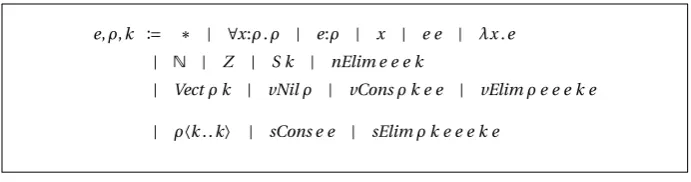
C.1 Syntax 92
1
·
Introduction
Earlier research has shown that functional languages and hardware can go, to some extent, hand in hand. The nature of hardware, easily thought of as a composition of computational blocks by means of wires, lies close to the nature of functional progamming, where the composition of functions is a fundamental operation. This has lead to the birth of variety of functional hardware description languages (HDLs), such as Lava [BCSS98], ForSyDe [SJ04], and CλaSH [Baa09, Koo09].
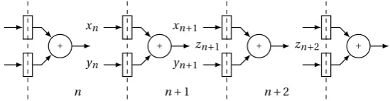
It is a property of all existing functional structural HDLs that they model hard-ware on a cycle-per-cycle basis: circuit blocks are defined by the computations they perform during a single clock cycle. For example, CλaSH models circuits as (com-positions of ) Mealy machines, with functions that act on an input and a state, and that return an output and a new state, on a per-cycle basis. However, the intended computations performed by circuits as a whole may span multiple cycles. It is not always obvious from a single-cycle description what the intended behaviour of the corresponding circuit is: the single-cycle descriptions obfuscate the multi-cycle com-putational essence of the circuits. If we want to understand what the circuit does conceptually, we may have to (mentally) simulate the circuit over multiple cycles. Given the complexity of present day hardware architectures, it will be clear that that is a cumbersome task and will give rise to errors. A definition that describes the multi-cycle behaviour of a circuit would be easier to understand, because it shows the intended computation directly.
This thesis is an initial attempt to provide an abstraction away from the single-cycle descriptions. With this abstraction, circuits can be defined on a higher level by their intended behaviour. Ideally, a translation mechanism might then take these definitions back to single-cycle descriptions, from which the hardware realisations can easily be extracted, for example, by the compiler CλaSH. A first task, however, is to check whether a composition of components, of which the overall behaviour is specified, can be synchronized correctly.
A similar attempt has been made by [Ott13], which introducestimed types. This notion separates a computation from its distribution in time: a circuit definition describeswhatneeds to be done, while its type specifieswhenit needs to be done.
Because moments in time (clock cycles) are naturally described by values (as opposed to types), it seems also natural to regard timed types as types depending on values. Such types are calleddependent types. The incorporation of dependent types into programming languages is a growing research topic, and may extend itself to hardware description languages.
The apparent resemblance of timed types to dependent types gives rise to our main research question:
so, how can we construct a type system, based on dependent types, that allows type checking of functional multi-cycle hardware specifications?
The perspective of this research question is different from the one taken in [Ott13], which is based on a constraint solving approach.
2
·
A beginning with dependent
types
This chapter will give a short informal introduction into dependent types. We start with Haskell-style types, and expand towards dependent types. This chapter is pro-gramming oriented, and is only meant to give a little taste of dependent types. For a more detailed exposition of dependently typed programming, we refer to appendix A, which discusses two dependently typed programming languages.
2.1 TYPES INHASKELL
Anyone who has programmed in Haskell is probably familiar with its type system. Every term has a type, which can be written asterm:type.1 There are base types, likeBoolandChar, and compound types which are built with other types, like the function typeChar→Booland the tuple type (Char,Bool).
Since Haskell is based on the Hindley-Milner type system, it also has so-called parametric polymorphic types[Jon03, DM82]. These types are parametrised by other types: they contain type variables, which can act as a type when multiple types are possible. For example, the identity functionidhas typea→a, whereais such a type variable. It means that the function can be used for values of any type. Haskell implicitly binds type variables with forall-quantifiers at the top level, such that the type ofidactually is∀a.a→a. Wheneveridis used, the type inference algorithm will try to find the actual type and substitute it fora. If, for example,idis applied to a boolean value,awill be substituted withBooland the type ofidbecomesBool→Bool.
Polymorphic types allow more abstraction and thus more flexibility. One can define a single list type without needing to be specific as to what type its elements should have. Similarly, one can write functions that act on every such list, regardless of the type of the elements — think of theheadfunction, which returns the first element of the list: it doesn’t really need to know the type of the elements. At the same time, polymorphic types are more specific: instead of having one generic list type that disregards the type of its elements, it is possible to create lists of booleans, lists of naturals, lists of strings, et cetera. With more specific types, more specific properties can be expressed, and with more specific properties, there is more confidence in the correctness of the program. Parametric polymorphism is therefore an important concept.
2.2 DEPENDENT TYPES
Parametric polymorphism allows types to depend on other types via type variables, but they cannot depend onvalues: it is for example impossible to create a list type where the length of the list, expressed as natural number, acts as parameter. In fact, in systems like Hindley-Milner, there is a strict separation between types and terms. Types can’t be used as values in functions, so is impossible to define operations on types like regular functions. In Haskell, it is possible to copy the behaviour of term values to the type level to some extent, to get natural numbers as types, for example, but this is quite tedious and seemingly redundant.
Dependent types do not have such a separation between terms and types. Types become terms and can use the same language constructs like lambda abstraction and application, so that it is possible to make functions that act on types. The relation between terms and types represented by ‘:’ becomes more general in a hierarchy of values, types, types of types, and types of types of types, etcetera. Every level of this hierarchy may depend on the same and all lower levels, and a type may therefore depend not only on other types, but also on values. Functions can now be generalised as dependent functions: because lambda abstractions are available for types, parameters can become actual arguments of functions. Dependent function types are of the form∀x:A.B(x), which says that the function takes anyxof typeA (which may be a type of types) to some typeBdepending onx. IfBdoes not depend onx, the type is equivalent toA→B. To illustrate, the type of the identity function can be written as
∀a:Type.∀x:a.a or ∀a:Type.a→a If the identity function is applied to some typeA, the result is
id A:A→A
such that the functionid Atakes any element of typeAto itself. Type signatures tend to become quite large if all quantifications are kept explicit. To keep the signatures concise, any quantification that can be inferred and that is not a function parameter can be made implicit, such that a valid type for the identity function is stilla→a. As a consequence, unbound variables occuring in types should be understood as bound by a forall-quantifier at top-level.
With dependent types, new possibilites arise to describe more precise properties of programs. The ‘list of certain length‘, or vector, is a common example. This type depends on the number of elements in the vector, such that a vector with three boolean values for example has typeVect Bool3. If it were a list, it would have type List Bool, which is the same type for all lists of booleans regardless of their length.
Similar to lists, there are two constructors for vectors. One is theNilconstant, which is defined to be the vector of length zero. The other constructor isCons, which puts some element in front of another vector, and therefore has an element and a vector as arguments. Both constructors are parametrised by types, so they need a type as argument. Because the result type ofConsdepends on the length of the vector argument (is is one element longer), it also needs that length as argument. The types of the constructors are therefore as follows:
Nil:∀a:Type.Vect a O
A bit of the power of dependent types becomes clear when two vectors are con-catenated. The vectors can have different lengths, and if they are concatenated, these lengths should be added together for the resulting type. Because types can depend on values, they can depend on terms that evaluate to values, liken+m(withnand mboth natural numbers). This makes it possible to guarantee that the length of the resulting vector is the sum of lengths of the argument vectors:
concat :Vect a n→Vect a m→Vect a(n+m)
concat Nil y = y
concat (Cons x xs) y = Cons x(concat xs y)
The+-operator in the type is just the ordinary operator acting on natural numbers. The body ofconcatdefines the concatenation recursively and with pattern match-ing, like it is commonly done for lists in Haskell: When the first vector is the empty vectorNil, the other vector is returned, and when the first vector is not empty (it is a Cons) then it takes the first element and puts it in front of the concatenation of the tail and the other vector. Notice that this definition uses the implicit notation. The explicit type ofconcatwould be
∀a:Type.∀n:N.∀m:N.Vect a n→Vect a m→Vect a(n+m)
The variablesa,nandmare quantified, and are therefore function arguments. They would have to be pattern-matched and explicitly passed around, to for exampleCons. However, because they can be inferred from the vector arguments, they can be made implicit, which removes a lot of clutter.
Another illustrative function with vectors isreplicate:
replicate :∀n:N.a→Vect a n replicate O x = Nil
replicate (S k) x = Cons x(replicate k x)
3
·
Type Theory
In the previous chapter we showed some examples with dependent types, and tried to bring some of its usefulness to light. In this chapter we will explore the theory. Through its history and foundations, functional programming is tightly bound to formal logic, and one of the goals of this chapter is to unveil this relationship. We will start with typeless first-order logic and introduce a version called constructive logic, which already has some computational elements. We then switch to the un-typed lambda calculus, which is the basis for many programming languages. By adding types to the lambda calculus, the set of allowable terms will be restricted, and we will show that the result corresponds to constructive first-order logic: lambda terms (programs) will be proofs, and propositions will be types. We will present this language first as the simply typed lambda calculus, which, with some extentions, matches to propositional logic, and then expand it to a dependently typed language, corresponding to first-order predicate logic.
We used several main sources for this chapter: [Tho91] gives introductory expo-sitions of logic and type theory; [End01] is an introduction to mathematical logic; [Bar93] gives a nice overview of lambda calculi with types, and seems to encompass most topics relevant to this chapter from the canoncical work [Bar84]. Finally, [ML84] has some nice informal explanations regarding type theory.
3.1 CLASSICAL AND CONSTRUCTIVE FIRST-ORDER LOGIC
3.1.1 Propositional logic
In this section we will describe a couple of formal logical systems. Such logical systems describe mathematical reasoning, in a very strict way. Mathematical ar-guments are considered as patterns of symbols, and any meaning we may give to those symbols is ignored. The correctness of the argument is embodied in theform of those patterns, such that it can be judged mechanically, without knowledge of their meaning. Manipulation of the argument can also be done entirely on just the patterns, because the formal system reflects the mathematical reasoning. Of course, in the end the result should be given an interpretation, so a formal system should include a way to give back the meaning to those symbols. In the following discussion, we do not separate form and meaning so rigorously. We do not need it for this thesis, and the forms are more easily understood with informal explanations.
“if ... then ...” to form an implication. If a statement cannot be split like this, we call it an atomic proposition.
To build compound statements from arbitrary statements, propositional logic introduces five connectives. Informally, these are “and”, “or”, “not”, “if ... then ...” (implication), and “if and only if” (bi-implication). In the realm of logical formulas we write them as∧,∨,¬,⇒, and⇔respectively. If we useAandBto denote arbitrary formulas, we can then for example writeA∧Band say that it is a formula.
Later on in this discussion, we will want to be able to refer within our proofs to a proposition that is always false. For this, we use⊥(falsum).
In short, we can now build formulas according to the following definition:
Definition 3.1.1. A formula is either:
• an atomic proposition denoted byX0,X1,X2, . . . , or
• a compound formula of the form (A∧B), (A∨B), (A⇒B), (A⇔B) or (¬A), whereAandBare formulas, or
• the falsum⊥.
If we are to use this definition exactly, we will have to write down a lot of paren-theses. When no ambiguity can arise, we will leave them out in favor of looks and clarity.
Formulas give us a way of writing down propositions. Some propositions, the axioms, we will accept without proof. Other propositions we will want to prove. If we succeed the proof, the proposition becomes a theorem.
A logical system lays down deduction rules for constructing proofs. These rules dictate how certain propositions may be inferred from others. Each rule therefore states what are the premisses, and what is the conclusion. A proof is then built by using these rules to infer new propositions from (possibly zero) previously inferred propositions.
In the following, we will use the natural deduction system, which allows to write down proofs in a very natural way. In this system, proofs are constructed in a tree-like structure, like this:
A B
C D
E
The root of the tree (E) is the proposition we want to prove. Each bar indicates the application of a rule: the premisses are above the bar, the conclusion is underneath. In the example aboveA,B, andDare premisses, andEis a conclusion.Cis both a premiss and a conclusion.
Above we said that the rules are used to infer new propositions from possibly zero previously inferred propositions. Most rules prescribe one or more premisses. One rule allows us to conclude propositions from nothing. These propositions are the assumptions we need for the proof, and the rule is therefore called the assumption rule. It says that to assume a proposition, we simply write it down:
A
assumptions hold. If the theorem is to be used in another proof, the assumptions will have to be accounted for in the new proof. Some rules allow certain assumptions to be discharged. This means that they do occur somewhere in the proof, but they do not have to be accounted for when using the theorem (they are discharged from their role as assumption). This happens when a rule has as premiss the fact that we can derive some proposition, and not the proposition itself. The use of discharged assumptions will become more clear when we discuss the individual rules.
To distinguish discharged assumptions from the other assumptions we will sur-round them with square brackets, and sometimes add labels to show at which steps they are discharged:
[A]1 B
1
C
The following rules are almost all related to the connectives. Either they introduce a connective into the argument (introduction rules), or they eliminate a connective (elimination rules) from it, allowing us to build up compound formulas and to extract sub-formulas.
∧-rules
Let’s start with the rules for∧-introduction and elimination:
A B
(∧I)
A∧B
A∧B
(∧E1)
A
A∧B
(∧E2)
B
The first rule, (∧I), is the introduction rule, and says that when we have two proposi-tionsAandB, we may also conclude their conjunctionA∧B. The other two rules are the elimination rules: they say that when we have a conjunction, we may infer either of its parts.
As an example, we can prove a part of the commutativity of the conjunction: if we assumeA∧B, we can deriveB∧A. We can do this by eliminating the conjunc-tion twice: once forAand once forB. We can then combine them again with the introduction rule:
A∧B B
A∧B A B∧A
In the natural deduction system every rule has only a single proposition as conclusion. Therefore, to concludeAandB, we have to use two assumptions. However, because they are the same, we may regard them as a single assumption.
Another example regards associativity. When we assumeA∧(B∧C), we can infer (A∧B)∧C. We first proveA,BandCwith the elimination rules:
A∧(B∧C) A
A∧(B∧C) B∧C
B
A∧(B∧C) B∧C
C
And then we can prove the goal with the introduction rule:
A B
∨-rules
The disjunction rules are as follows:
A (
∨I1)
A∨B
B (
∨I2)
A∨B A∨B
[A] .. . C [B] .. . C
(∨E)
C
We now have two introduction rules. The first says that when we haveA, we may conclude ‘Aor something else’. The second says the same, but with the disjuncts swapped. The elimination rule is a bit more complicated. Here we see the first use of discharged assumptions. The rule says that when we knowA∨B, and we can proveC once by assumingAand once by assumingB, we can concludeC. In other words, as long as we know thatCcan be proved for both assumptions independently, we can concludeCdirectly fromA∨B. We do not need to prove which ofAandBis true: according to the premisses, at least one of them is true, andCwill hold either way. That means that the conclusion only depends on the assumptionA∨B, and not on the assumptionsAandB. Therefore,AandBcan be discharged. Should we want to useCin another proof, then we only need to takeA∨Binto account as assumption.
As an example, we can use again the commutativity property:
A∨B
[A]1
B∨A
[B]1
B∨A
1
B∨A
Using the introduction rules we can proveB∨Afrom bothAandB, and therefore we can use the elimination rule to concludeB∨AfromA∨B.AandBare discharged by the elimination rule, so we have provedB∨Afrom the single assumptionA∨B.
⇒-rules
The implication rules are as follows:
[A] .. .
B (
⇒I)
A⇒B
A A⇒B
(⇒E)
B
The introduction rule states that if we can deriveBfromA, we can conclude thatA impliesB. The elimination rule says that if we know thatAimpliesB, and if we know Aholds, we can conclude thatBholds.
The conclusionA⇒B does not depend on whether or notAholds, the only premiss is thatBisderivablefromA. Therefore,Ais discharged in the introduction rule. This does not mean that we can’t use other assumptions in the derivation ofB, but the conclusion will depend on them as well if we do. In the elimination ruleA does become a proper assumption, because now we use it together withA⇒Bto deriveB.
As an example, we use the transitivity property of implication. If we assume A⇒B, andB⇒C, then we can concludeA⇒C:
[A]1 A⇒B
B B⇒C
C
1
Here we used the elimination rule twice to derive firstB and thenC, under the assumptionsA,A⇒BandB⇒C. Since we derivedC fromA, we can conclude A⇒C with the introduction rule. The conclusion does not depend anymore on whetherAholds or not: we have proved thatifit holds, thenCholds as well, which is what we understand as implication. The assumptionAcan therefore be discharged. Of course, the other assumptions are still necessary.
Note that we could remove the remaining assumptions from the proof by using the implication rule. This would leave us with a tautology:
[A]1 [A⇒B]3
B [B⇒C]2
C
1
A⇒C
2
(B⇒C)⇒(A⇒C)
3
(A⇒B)⇒((B⇒C)⇒(A⇒C))
⇔-rules
Bi-implication is very similar to implication:
[A] .. . B
[B] .. . A
(⇔I)
A⇔B
A A⇔B ( ⇔E1)
B
B A⇔B ( ⇔E2)
A
To introduce bi-implication, Aneeds to be derivable fromB andB needs to be derivable fromA. We can eliminate bi-implication using eitherAorBas premiss, and concludingBorArespectively.
¬-rules and⊥
Before discussing negation, we will take a look at⊥. This is the symbol to denote absurdity or contradiction. We can regard it as a proposition that is always false, and it should therefore be impossible to prove. If we can prove⊥, we can prove anything. This notion is embodied by the following elimination rule:
⊥ (⊥E) A
We cannot introduce⊥, because it is impossible to prove. However, we can use it to define negation, because ifAdoes not hold, any proof ofAleads to a contradiction:
¬A≡A⇒ ⊥
With this definition and the⊥-elimination rule, we can derive the rules for¬ -introduction and elimination. Elimination can be done by using a contradiction: if we have bothAand¬A, we can conclude⊥, and the⊥-elimination rule subsequently allows us to prove anything. This becomes clear if we use the implicative form of the negation:
A A⇒ ⊥
(⇒E) ⊥ (⊥E) B
A ¬A
(¬E)
B
To introduce a negation, we want to show that the assumptionAleads to⊥(since that is the definition). If we assumeAand derive bothBand¬B, we conclude⊥, like we did earlier. The implication rule then allows us to concludeA⇒ ⊥, or¬A:
[A]1 .. . B
[A]1 .. .
B⇒ ⊥ (⇒E) ⊥
1 (⇒I)
A⇒ ⊥ Again we can turn this into a concise rule:
[A] .. . B
[A] .. . ¬B
(¬I) ¬A
At the beginning of this section we said that classical propositional logic concerns statements that are either true or false. It implies that there is no grey area between true and false. This principle is called ‘the law of the excluded middle’. A consequence of this law is that if we can prove that a statement is not false, we may conclude it is true and vice versa. By definition, we can conlude¬AwhenAbrings us to a contradiction. If we replaceAwith¬A, we can conclude¬¬Awhen¬Adoes not hold. However, we have no rules yet to concludeAfrom not¬A. In other words: the law of excluded middle does not hold. To remedy this, we can add one or more of the following equivalent rules.
First, we can introduce the law as an explicit rule:
(LEM)
A∨ ¬A
We can also choose a rule in which we concludeAfrom¬¬A, called the rule of double negation:
¬¬A
(DN)
A
Finally, we can also introduce a rule similar to the introduction rule (¬I). Instead of deriving a contradiction fromAand concluding¬A, we assume¬Aand conclude A. This is the classical proof by contradiction:
[¬A] .. . B
[¬A] .. . ¬B
(CC)
A
3.1.2 Predicate logic
In the propositional logic of the previous section, the only objects of interest were propositions. In a mathematical discourse we generally also recognise other kinds of objects, and we make statementsaboutthese objects. For instance, the statement “42 is even” asserts that the number 42 has the property that it is even, via the predicate “is even”. If we extend propositional logic with the means to reason about objects and
their properties, we get predicate logic.
Definition 3.1.2. A term is either:
• a constant (we will usea,bandcfor arbitrary constants),
• a variable (we will usex,yandzfor arbitrary variables), or
• a function of arityn,n>0, applied tonterms (we will usef,gandhto denote arbitrary functions, and write applications as for examplef(x,y)).
If we refer directly to an object, we call the term a constant. For example, we associate the term 42 directly with the number 42, much like how we associate the name Bertrand Russell with a particular polymath. We can also refer to arbitrary objects, with variables. In the sentence “xis prime”, the termxcan point to any object. However, a variable will (within boundaries we will discuss later) always point to the same object: In “xis prime andxis even”, thex’s denote the same object, while in “xis prime andyis even”, the objects ofxandymay be different. The last kind of term is the function, which allows us to use objects to refer to other objects. For example, the termx+4 points to the object we get from adding 4 tox.
We have now defined how we represent objects within predicate logic. If we combine them with predicates, we get atomic propositions: LetP be an arbitrary n-ary predicate (n>0) and lett1,t2, . . . ,tnbe terms.P(t1,t2, . . . ,tn) is then an atomic proposition. For example, ifPis the binary predicate “is greater than”, thenP(7, 4) means “7 is greater than 4”. When we encounter common predicates like this, we will use the regular notation, e.g. 7>4.
From atomic propositions, we can again build formulas:
Definition 3.1.3. A formula is either: • an atomic proposition
• a compound formula of the form (A∧B), (A∨B), (A⇒B), (A⇔B) or (¬A), whereAandBare formulas, or
• a quantified formula of the form∀x.Aor∃x.A, whereAis a formula andxis a variable.
The formulas are constructed similarly to propositional logic. The new elements are formulas with the universal quantifier∀(for all) and the existential quantifier∃ (exists). These quantifiers allow us say something about the extent to which predi-cates are valid: Say we have the non-quantified propositionx>3. This proposition says that whatever objectxrefers to (we limit ourselves to the natural numbers), this object at least satisfies the predicate>3. When we add a quantifier, we don’t say something about the objectxitself, but about the range of objects for which the proposition holds. If we write∀x.A, we say that propositionAholds no matter what object we choose forx: “for allx,Aholds”. Therefore, if we write∀x.(x+1)>0, we say that whatever we choose forx, it will be true that (x+1)>0. Similarly, if we write ∃x.A, we say that there is at least one object for which the propositionAholds: “there exists anx, such thatAholds”. For instance,∃x.x>3 means that there is at least one objectxsuch thatx>3.
yis not bound: we call it a free variable. When a quantifier binds a variable that has already been used, the newly bound variable holds no relation to the old one. So in (x>2)∧(∀x.∃y.y>x)∧(x<4), the first and fourthxare free and refer to the same object. The third one is bound, and is independent of the otherx’s. The same goes for nested quantifiers: in∃x.(x>3∧ ∃x.x<10), the secondxis bound to the first quantifier, while the fourthxis bound to the second quantifier.
The rules from propositional logic also apply to predicate logic. We only need to add rules for the quantified formulas. We again have an introduction rule and an elemination rule for each quantifier.
∀-rules
These are the rules for∀-introduction and elimination: A
(∀I) ∀x.A
∀x.A
(∀E)
A[x:=t]
The elimination rule (∀E) introduces a new notation: We useA[x:=t] to say that in the formulaA, all free occurences ofxmust be substituted with the termt. This definition alone invites a problem:tmay contain variables that become bound inA. Take for example the proposition∃x.x>y. We could substituteywith a free variable x, different from the boundx:
(∃x.x>y)[y:=x]
This results in the proposition∃x.x>x, where suddenly the freexwe substituted becomes bound as well. This phenomenon is called variable capture. Since bound variables are dummies used for the quantification, we can replace them with other variables:∃x.x>y means the same as∃z.z>y. We can therefore avoid variable capture by changing the quantification variables to “fresh” variables if they also occur int. We can make the above definition more rigorous by accounting for variable capture, but we postpone the effort and assume we always use unique variables, keeping in mind that we can always rename bound variables if necessary.
Now that we know substitution, we can explain the elimination formula: it says that when a propositionAholds for allx, we can replacexwith any other termt. For example (we limit ourselves again to the natural numbers):
∀z.z2>0 (x+y)2>0
Ifz2holds for allz, then we can choosex+yforz, wherexandyare fresh variables. Whatever numbersxandyare, the square of their sum is greater than or equal to 0, because the square of every natural number is greater than or equal to 0.
The introduction rule (∀I) states that if we have provedA, we have provedAfor all x. Application of this rule calls for some caution, because there is a restriction on the use ofxin the derivation ofA:xmay not appear free in any of the assumptions (that includesAitself, if it is an assumption). This is called the side condition of the rule. Consider what happens ifxappears free in one of the assumptions: In that case, the assumption states some property that must hold ofx. Although we may not knowx, it can only be one of those objects that satisfy the assumption. Therefore we cannot conclude thatAholds for all objects. For example, ifAwould be the assumption x>10, we clearly can’t conclude∀x.x>10.
∀z.z2>0 (x+y)2>0 ∀y.(x+y)2>0 ∀x.∀y.(x+y)2>0
This proof shows how we can use the quantified variables of the conclusion free in the derivation. In this case,xandyare names for unknown objects, introduced via the∀-elimination rule. Because we don’t make assumptions aboutxandy, we may conclude that they may range over all objects, such that∀x.∀y.(x+y)2>0.
∃-rules
These are the rules for the existential quantifier:
A[x:=t]
(∃I)
∃x.A ∃x.A
[A[x:=a]] .. . B
(∃E)
B
The introduction rule again mentions substitution. It says that if the proposition Aholds whithtsubstituted forx, then there exists anxsuch thatAholds. A small example:
2<3 ∃x.x<3
We know that 2<3, so we know that there exists anxsuch thatx<3.
The elimination rule says the following: if we know that there exist one or more xsuch thatAholds, and fromA[x:=a] we can deriveB, we may concludeB. The premiss∃x.Aguarantees the existence of an object such thatAholds. Because we don’t know for which object(s)Aholds, we cannot derive anything directly from it. To be able to useA, we can pretend to know the object and give it a fresh name, for examplea(for the purposes of this chapter, we’ll call a name fresh if it hasn’t been used earlier in the proof ). We may then assumeA[x:=a] holds, and use it to prove B. The premiss∃x.AjustifiesA[x:=a], so we may discharge this assumption, and concludeBjust from∃x.Aand its derivability fromA[x:=a].
However, like the∀-introduction rule (∀I), this rule needs some caution. Besides the requirement ofabeing fresh, there are two other side-conditions that concern the use ofa. The first condition is thatashould not appear free inB, which leads to trouble when we discharge the assumption. Consider the following derivation:
∃x.x<3
[a<3] .. .
a<4 (wrong!!) a<4
This derivation says that we can provea<4 merely from the fact that∃x.x<3. In the subderivationais not arbitrary: we assumeda<3. However, this assumption is discharged when we apply the rule.ais then an arbitrary object, and it is clearly incorrect to say that an arbitrary object is less than four because there exists some object less than three.
If we ignore this condition, we are assuming more aboutathan is justified by∃x.A. We cannot discharge these assumptions, and as a consequenceBstill depends on assumptions abouta. When these assumptions are more strict thanA[x:=a] (so that the objects that make these assumptions together hold are a subset of those that makeA[x:=a] hold), we don’t rely on∃x.Aat all, because the existence of those objectsxis implied by our stricter assumptions. If the assumptions are less strict, we run into similar problems as when we allowato be free inB:
∃x.x<3
[a<3] a>1
.. . a=2 ∃y.y=2
(wrong!!) ∃y.y=2
Here we have “proved” that we can conclude∃y.y=2 from the assumptions∃x.x<3 anda>1, which is clearly wrong: we also needa<3 to conlude∃y.y=2.
3.1.3 Constructive logic
Up to this point, we regarded propositions as statements that can only be either true or false. We embedded this principle in our propositional logic at the end of section 3.1.1 as the rule of the excluded middle:A∨¬A. To use this rule, we can apply ∨-elimination: we prove some other propositionBonce by assumingAand once by assuming¬A. If we succeed both proofs, we have provedB. A classical example is a proof that there exist two irrational numbersaandbsuch thatabis rational. We start with the LEM,
p 2
p
2
is rational orp2 p
2
is not rational,
and proceed to prove the hypothesis for both cases:
• Assumep2 p
2
is rational. Leta=p2 andb=p2. Thenab=p2 p
2
, which we assumed rational, so in this case there are an irrationalaandbsuch thatabis rational.
• Assumep2 p
2
is irrational. Leta=p2 p
2
andb=p2. Thenab=p2 p
2p2 =p22, which is rational, so in this case too there are an irrationalaandbsuch thatab is rational.
Since in both cases we have found anaandbsuch thatabis rational, we have proved the hypothesis.
This proof does not depend on knowing whether or notp2 p
2is rational. While the
law of the excluded middle says it’s one or the other, our interpretation ofA∨Ballows us to leave undecided which one it is exactly. We can therefore prove the existence of a, without knowinga.
a construction, and that we can use this construction in a further line of proof. In a similar vein, proofs themselves form constructions, as shown by what is now called the BHK-interpretation of Brouwer, Heyting and Kolmogorov:
• A proof ofA∧Bconsists of a proof ofAand a proof ofB.
• A proof of A∨B consists of a proof ofAor a proof ofB, together with an indication of which proof it is.
• A proof ofA⇒Bis a method to turn a proof ofAinto a proof ofB. • A proof of∃x.Aconsists of the construction of aaand a proof ofA[x:=a]. • A proof of∀x.Ais a method to turn a construction ofainto a proof ofA[x:=a]. • A proof of¬Ais a proof ofA⇒ ⊥.
• A proof of⊥does not exist.
When we assumeA∧B, we may conclude eitherAorB. In a constructive setting this means we need proof of bothAandBto concludeA∧B. In classical logic a proof of ¬(¬A∨¬B) can be used to proveA∧B, but since this provides no proofs ofAandB, it is not a generally valid method in constructive logic. Similarly,A∨Brequires a direct proof of eitherAorB, which is not implied by the classically equivalent¬(¬A∧ ¬B). A constructive proof of implication should show that any proof of the first propo-sition in some way also justifies the second: it is a method to transform the proof of one into a proof of the other. The proof of a universally quantified proposition is likewise a method, but now from objects to proofs. A proof of a proposition is built from facts implied by the construction of an object; a universal proof is a method to provide such a proof for any object.
As the constructive interpretation rejects indirect proofs, it also rejects the law of excluded middle and its siblings. The assertionA∨ ¬Arequires either a proof ofAor a proof of¬A. As long as there is no proof of either (i.e. a problem is unsolved),A∨¬A cannot be asserted. Similarly¬¬Aonly asserts that¬Aleads to a contradiction. It does not provide a direct proof ofA, so the law of double negation also cannot hold in general.1
3.2 LAMBDA CALCULUS
In the previous section we looked at logic, and arrived at a version with a compu-tational nature. In this section we will start with a compucompu-tational formalism, and work towards a union of logic and computation. The computational formalism is the untyped lambda calculus, which was actually part of a formal logic proposed by Alonso Church in the 1930s. This logic was proved inconsistent by two of his students, after which Church excised the calculus and combined it with ideas from the theory of types, resulting in the simply typed lambda calculus. Starting in the late 1950s, the lambda calculus started influencing the development of programming languages, and eventually lead to languages like ML, and later Haskell. However, the relation to logic was not entirely lost. In the 1960s, De Bruijn and Howard independently posited interpretations of terms as proofs and types as propositions. This resulted in proof checking systems like for example AUTOMATH. The mathematical and programming
communities influenced each other, and many different calculi and type systems evolved. [CH09, Bar93]
In this chapter, we will start with the untyped lambda calculus, and expand it first to the simply typed lambda calculus, and then to a system with dependent types, while also highlighting the logical interpretation.
3.2.1 Untyped lambda calculus
The lambda calculus is a function oriented calculus. Its only objects are functions, and at its heart it is concerned only with the construction and use of these objects. A function can be constructed with abstraction: in a common mathematical context we may seef(x)=x+2 as a generalisation of for instance the operation 5+2, where we abstracted from the particular number we added to 2. When we have such a function, we can use it by applying it to some argument: f applied to 3, written f(3), is to mean the particular operation 3+2. In the pure lambda calculus, application and abstraction are the key ingredients. In fact, together with variables, they are the sole ingredients, as we can see in its syntax:
Definition 3.2.1. The syntax of the pure lambda calculus is: t :=v |λv.t |t t
The categoryvrepresents the variables; we will use letters near the end of the alphabet for them (x,y,zan the like). The abstraction of a termeover variablexis written asλx.e. The application of a termf to a termeis written asf e.
To keep the notation concise yet unambiguous, we will adhere to the following rules: applications associate to the left, and parentheses are used when necessary to delimit lambda-abstractions and applications. Thusx y cwill mean (x y)z(the application ofx ytoz), which is different fromx(y z) (the application ofxtoy z), andλx.x yis an abstraction ofx y, while (λx.y)zis the termλx.yapplied toz.
A lambda-abstraction indicates a parameter of a term. Inλx.t,xis a parameter of the termt, and we say that it isbound. If a variable occurs intnot bound, then it occursfree. If a term contains free variables we call itopen, and if it contains no free variables we call itclosed. Soλy.x yis an open term, becausexis free, whereas λx.λy.x yis closed because bothxandyare bound. Because a bound variable is a formal parameter, we can change its name without altering the meaning of the term: the functionλx.xwill do the exact same thing asλy.y. We will therefore regard such terms as equal.
As we mentioned above, when we writef(3), the application off to 3, we actually intend to substitute 3 for the parameter in the definition off. When we have defined f(x)=x+2,f(3) simply means 3+2. We can say thatf(3)reducesto 3+2. Of course,+ itself is also a function, and we could substitute 3 and 2 for the respective parameters of whatever the definition of+is. In the end, we would expect 3+2 to reduce to 5. This process of reduction is reflected in the lambda calculus by the so-calledβ-reduction rule:
Definition 3.2.2. β-reduction:
(λy.t1)t2→βt1[y:=t2]
It says that when we encounter a lambda-abstractionλy.t1applied tot2, we may
symbol→βcan be read as “reduces to”. For example, (λx.x)y→βy
says that the identity function applied toyreduces toy. We will call a term of the form (λy.t1)t2a reducible expression (redex), and the reduced formt1[y:=t2] the
reduct.
The lambda calculus does not allow functions with multiple parameters. However, it is possible to represent such functions by means of currying: we can abstract a term repeatedly to add the parameters, such that it becomes a function of one parameter which returns another function of the next parameter, which returns another function et cetera. For example, we may view the functionλx.λy.xas having two parameters, while it is in fact a function with parameterx that returns another function with parametery:
(λx.λy.x)u→βλy.u
We can make use of repeated applications to supply all arguments:
(λx.λy.x)u v→β(λy.u)v→βu
In the following, we will useto denote multiple reductions, such that we can abbreviate the above sequence as
(λx.λy.x)u vu
We will use the same symbol to denote reductions that occur within an expression:
λx. (λy.z)xλx.z
When a term cannot be reduced any further (it contains no redexes), it is innormal form. Every term has at most one normal form: normal forms are unique. Fur-thermore, if a term has a normal form, it can be reached by repeated reduction [Bar93]. However, not every term has a normal form. A canonical example is the term (λx.x x) (λx.x x), which reduces to itself.
As we reduce a term, its meaning as a whole does not change. Therefore, if two terms have the same normal form, they have the same meaning. This leads to a notion ofβ-equality (sometimes called convertability):
Definition 3.2.3. β-equality:
If two termst1andt2have the same normal form, i.e. there exists a non-reducible
termtsuch thatt1tandt2t, then we call themβ-equal:
t1=βt2
For example, we have (λx.x)y =β(λx.y)z. Note that terms that do not have a normal form are also not equivalent to any other term.
The lambda-calculus so far may seem limited, but it is nevertheless turing com-plete. We will give two basic examples of programming in the untyped lambda calculus, involving booleans and natural numbers. To represent the boolean values “true” and “false”, we can use the following definitions:
We can think of them as functions of two parameters, where true always returns the first, and false always returns the second parameter. We can define some of the usual boolean functions based on this selective behaviour as follows:
not≡λx.x false true and≡λx.λy.x y false
or≡λx.λy.x true y
If we applynotto true andfalse, we get the following reduction sequences:
not true→βtrue false true→β(λy.false)true →β false not false →βfalse false true →β(λy.y)true→β true
The other functions work in a similar way.
Natural numbers can be encoded as so-called Church numerals:
0≡λf.λn.n 1≡λf.λn.f n 2≡λf.λn.f(f n) 3≡λf.λn.f(f(f n))
.. .
So a numberxis represented by a function that makes a composition ofxapplications of the first argumentf and applies that composition to the second argumentn. If we viewf as a “successor” andnas “zero”, we can see a resemblance to the Peano representation of the natural numbers.
An actual successor function for Church numbers would be
succ≡λx.λf.λn.f(x f n)
Given a numberx, it returns another function with argumentsf andn. It appliesx tof andnto get thex-fold composition off applied ton, and thenf is applied to the result to get the actual successor. For example:
succ0→βλf.λn.f (0f n)→βλf.λn.f((λn.n)n)→βλf.λn.f n Addition can be done in a similar manner with
add≡λx.λy.λf.λn.x f (y f n)
This function first applies they-fold composition off ton, and then, instead of just a single application off, it applies thex-fold composition off to the result, leading to the (y+x)-fold composition off applied ton.
Our last demonstration of the untyped lambda calculus is the powerful concept of recursion: functions defined in terms of themselves. Famous examples are functions that calculate factorials and Fibonacci numbers:
fac0≡1 fib0≡0
fac n≡n·fac(n−1) fib1≡1
In the pure lambda calculus we can’t use the term we are defining within itself, but we are not prohibited to apply a term to itself. We have already seen the term
(λx.x x) (λx.x x)
which reduces to itself. A similar term from the mind of Alan Turing is
Y ≡(λy.λf.f(y y f)) (λy.λf.f(y y f))
This term is a bit more complicated, but it can be quickly checked that for every functionf we have
Y ff (Y f)f (f (Y f))· · · Now suppose thatf has the formλg.λx. (· · ·g· · ·), such that
Y f f (Y f)λx. (· · ·(Y f)· · ·)
The termY f now reduces to a function that contains itself: it is a recursive function. As a more concrete example, here is a definition of the factorial function:
rfac0 ≡λf.λn.if(n=0)then1else n·f (n−1) rfac≡Y rfac0
We sugar-coated it a bit with some arithmetic operators and a test for zeroness, but it is nevertheless expressible in the pure lambda calculus. TheY-function effectively replacesf inrfac’withrfac, such thatrfacbecomes the factoriol function as we know it.
3.2.2 Simply typed lambda calculus
The untyped lambda calculus is powerful, but it has some peculiarities. We have seen in the previous section that it is capable of representing booleans and natural numbers, but it is also very well possible to write terms likesucc add false, which have little meaning to us. We perceive booleans, natural numbers, and the functions acting on them as different concepts, which are not necessarily interchangeable.
To fix this peculiarity we can divide terms into types, and introduce rules that limit how we can use terms of different types. The language of types, like that of the lambda calculus, is simple:
Definition 3.2.4. The syntax of simple types is: T :=B |T→T
Every allowable term will have a type in the prescribed form. We can say that a term has some type if we can derive the type from (the types of ) its subterms with the typing rules we will discuss. Because variables do not have subterms they appear at the top of the derivation tree. We can’t derive the types of variables, so we have to assume their types. As a consequence, a term only has a type for a certain set of type assumptions. We call this set thecontext. To express that a termthas a typeτ, we will write
t :τ
and to say that termthas typeτin contextΓ, we write
Γ`t:τ
During the typing derivation we will want to alter the context, so we can for example create a different context by adding a new assumption:
Γ;x:σ
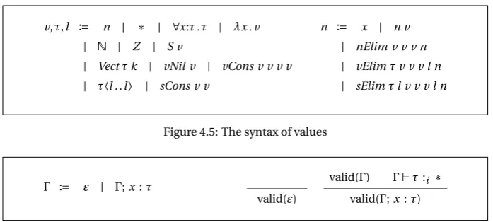
forms a new context that consists of all assumptions fromΓand the new assumption x:σ. For a context to be valid, we require that each assumption consists of a variable and a type with proper syntax (a well formed type).
Now we come to the typing rules. We borrow the notation of natural deduction:
Definition 3.2.5. The typing rulesvar,lam, andappare: x:τ∈Γ
Γ`x:τ
Γ;x:σ`e:τ
Γ`λx:σ.e :σ→τ
Γ`e1:σ→τ Γ`e2:σ
Γ`e1e2:τ
The rule for variables (var) expresses that ifx:τis an assumption in contextΓ, we may conclude that given contextΓ,xhas typeτ. The lambda abstraction rule (lam) tells us that in order to build a lambda abstractionλx:σ.eof typeσ→τ, we need to have a termeof typeτunder at least the assumptionx:σ. By abstracting overxwe turn it into a parameter of typeσ, so we can removex:σfrom the context. Often it is clear what the type ofxshould be; in such cases we will omit the type and write λx.e. Finally, the application rule (app) states that the result of an applicatione1e2
has typeτife1is a function with a domain of typeσand a range of typeτ, and the
type of argumente2matches the domain typeσofe1, all under contextΓ. Note that
these typing rules only hold under the assumption that the contexts are valid (i.e. all elements of the contexts are variables with well formed types, as discussed above).
The following derivation example contains all three rules:
f :σ→τ∈Γ
(var)
Γ`f :σ→τ
x:σ∈Γ
(var)
Γ`x:σ
(app)
Γ`f x:τ
(lam)
x:σ`λf.f x: (σ→τ)→τ where we used
Γ≡x:σ; f:σ→τ
with the application rule, and subsequently abstract over f with the lambda rule, wheref disappears from the context as it becomes bound.
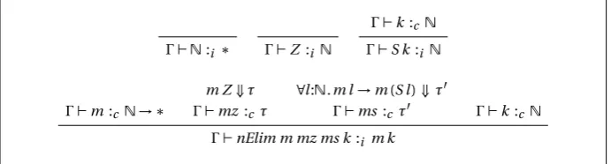
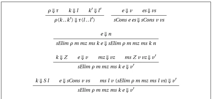
The simply typed lambda calculus so far does not have any meaningful base types, so we will extend it. We will add the typeNfor natural numbers. Because the definitions we gave in the previous section of the values of these types are not really intuitive, we will also add a couple of new terms that seem to make more sense, namelyZfor zero andSfor the successor function. To make sure that these terms have the proper types, we introduce some new typing rules:
Γ`Z :N
Γ`k :N
Γ`S k :N
We may always conclude that zero is a natural number, and ifkis a natural number, we may conclude its successor is one as well. Besides creating natural numbers, we also want to use them. For this we introduce the termnatElim, which will allow us to perform recursion over the natural numbers. Its typing rule is
Γ`e0:τ Γ`f :N→τ→τ Γ`k :N
Γ`natElim e0f k:τ
The terme0is the base case of the recursion, andf is the step function. The behaviour
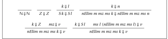
ofnatElimis perhaps best explained with its reduction rules:
natElim e0f Z→e0
natElim e0f (S k)→f k(natElim e0f k)
When the last argument isZ, we are in the base case and returne0. When it is a
successor ofk, we returnf applied to bothkand the result of the previous recursion step. As an example, we can implement the factorial function (we assume that we have a multiplication on natural numbers):
fac ≡λn.natElim(S Z) (λk.λr. (S k)·r)n WhennisZ, this reduces toS Z. WhennisS kwe get
(λk.λr. (S k)·r)k(fac k) which reduces to
(S k)·(fac k) as we would expect from the factorial function.
3.2.3 Propositions as types
trees become typing derivations, and that proofs become terms. In this section we will explore this dual view.
The simply typed lambda calculus cannot yet accomodate all connectives we have described for the propositional calculus (§3.1.1), so we will have to extend it. This is partly a repetition of section 3.1.1, because we will have to describe what are valid types (formulas) and what are the typing rules (introduction and elimination rules). The new component is that we also describe new terms, which we will use to construct the proofs of the propositions, and new reduction rules that come with such terms, which describe how can we convert one proof of a proposition to another. We will trot deeper into these concepts as we go along, but first we will look at the single connective the calculus already supports: implication.
A lambda-abstraction represents a method to turn terms of one type into terms of another. This conforms exactly to the BHK-interpretation of a proof of implication, which is a method to turn the proof of one thing into a proof of another. When we read the typing rules of lambda abstraction and application as deduction rules, we see that they resemble the introduction and elimination rules. Compare for example the introduction and lambda abstraction:
[A] .. .
B (
⇒I)
A⇒B
Γ;x:σ`e:τ
(lam)
Γ`λx.e:σ→τ
To introduce an implicationA⇒B, we need to show that we can derive proposition Bfrom the assumptionA. To introduce a term of typeσ→τ, we need to show that we have a term of typeτunder the assumption that we have a term of typeσ. The structures are equal. The main difference between the rules is that the typing rules also tell you what a proof looks like: the proof ofσ→τis a lambda-abstraction, a method, which takes one proof to another.
When we look at elimination and application, we see a similar congruence: To eliminate an implicationA⇒B, we need a proof ofA, and we conclude that we have a proof ofB. When we have a term of typeσ→τand a term of typeσ, the application of the first to the second gives us a term of typeτ:
A A⇒B ( ⇒E)
B
Γ`e1:σ→τ Γ`e2:σ (app)
Γ`e1e2:τ
Considering the similarities we saw, it is not a giant step to read→as the implicational connective.
Aside from the types, terms and typing rules, the lambda calculus also gives us a reduction rule:
(λx.t1)t2→βt1[x:=t2]
This rule is a transformation between proofs: it preserves type, but changes the proof. Notice that the term (λx.t1)t2is a lambda-abstraction followed by an application,
which means that as a proof, it introduces an implication which is subsequently eliminated, forming a sort of detour. The reduction rule translates this detoured proof into a more direct one.
by adding terms of the form (t1,t2), which then have the type (σ∧τ). Because we
can only build a proof of (A∧B) when we have proofs of bothAandB, we can only construct a term of type (σ∧τ) if we have a term of typeσand a term of typeτ:
Γ`t1:σ Γ`t2:τ
Γ`(t1,t2) : (σ∧τ)
This rule corresponds to the∧-introduction rule. We also need the corresponding elimination rules, which say that we may extract the subproofs to prove the subpropo-sitions: from (A∧B) we can proveAandBindividually. Since a proof of (A∧B) is a pair of subproofs, we can extract the right subproof if we want to concludeAorB. In the lambda calculus this means we have to add two new termsπ1tandπ2t, which,
given a term (t1,t2) : (σ∧τ), extract the corresponding subtermst1andt2. This is
reflected in the reduction rules we add:
π1(t1,t2)→t1 π2(t1,t2)→t2
The typing rules forπ1andπ2are then
Γ`t: (σ∧τ)
Γ`π1t:σ
Γ`t: (σ∧τ)
Γ`π2t:τ
As an example, let’s look at the following derivation:
Γ≡x:σ∧τ; f:σ→ρ
Γ`f :σ→ρ
Γ`x:σ∧τ
Γ`π1x:σ
Γ`f(π1x) :ρ
x:σ∧τ`λf.f(π1x) : (σ→ρ)→ρ `λx.λf.f(π1x) : (σ∧τ)→(σ→ρ)→ρ
Here we have a type derivation of a function which takes a pairxand some function f, and returnsf applied to the first element ofx. This is similar to having a proof that σ→ρimpliesρifσ∧τhold. This proof then constitutes the method of transforming the proof ofσ, that is included in the proofxofσ∧τ, to the proof ofρ, usingπ1and
the methodf that provesσ→ρ.
Besides conjuntion we also have disjunction: a proposition (A∨B), which is proved by either a proof ofAor a proof ofB, plus an indication of which proof it is. In functional languages, we may view disjunctions as disjoint unions of datatypes, as for instance theEithertype in Haskell:
data Either a b=Left a|Right b
This type represents the disjoint union of the typesaandb: the contained values may be of either type, while the constructorsLeftandRightindicate which of the two it is.
We will include the disjunction in the extended lambda calculus as types of the formσ∨τ. To introduce terms of such a type we add two new forms:in1tandin2t.
If we regard them both of typeσ∨τ, then the first form indicates thattis of typeσ, while the second indicates thattis of typeτ:
Γ`t:σ
Γ`in1t:σ∨τ
Γ`t:τ
To eliminate a disjunction, we need to show we can prove another proposition from either disjunct. We had the following elimination rule:
A∨B [A]
.. . C
[B] .. . C
(∨E)
C
We can express the fact thatCis derivable fromA(orB) asA⇒C(orB⇒C), so the above rule is equivalent to
A∨B A⇒C B⇒C C
We can now easily translate the premisses to typing judgements, but we don’t yet know exactly what a proof ofClooks like. It depends on the proof of A∨B: If we havein1t, thenCis proved by applying the proof ofA⇒C(the second premiss) to t, which is the proof ofA. IfA∨Bis proved byin2t, thenCis proved by applying
the proof ofB⇒C(the third premiss) tot(which is now a proof ofB). Because we don’t know on beforehand which case we are in, we add another term to express the options:case t f g. Here,tis our disjunction, f is the proof ofA⇒C, andgis the proof ofB⇒C. Ifthas the formin1t1it will reduce tof t1, and if it has the form
in2t2it will reduce tog t2:
case(in1t1)f g→f t1
case(in2t2)f g→g t2
With this new term, we can express the elimination rule as a typing rule:
Γ`t:σ∨τ Γ`f :σ→ρ Γ`g:τ→ρ
Γ`case t f g:ρ
The last connective we will discuss is⊥. This is the absurd proposition, which has no proof, and therefore no introduction rule. In the lambda calculus, this means that there is no value of type⊥. If any computation has type⊥, it can therefore never return a value: either it never halts, or it is inherently erroneous. However, we did have an elimination rule, which said that by proving⊥, we could prove anything. As a typing rule, this means that if we do have a term of type⊥, we can introduce a term of any type. A term that can have any type voids any computation that depends on it of its meaning, and we might as well abort the computation. This suggests an interpretation of the “term-of-any-type” as a primitive to raise errors, and we may use for example the following typing rule:
Γ`t:⊥