A Thesis Submitted for the Degree of PhD at the University of Warwick
http://go.warwick.ac.uk/wrap/49963
This thesis is made available online and is protected by original copyright. Please scroll down to view the document itself.
RNA-seq and ChIP-chip data
Author: Nigel P. Dyer
A thesis submitted to the University of Warwick for the degree of
Doctor of Philosophy
Supervisors: Dr Sascha Ott and Professor Jim Beynon
Molecular Organisation and Assembly in Cells (MOAC)
Doctoral Training Centre
List of tables... viii
List of figures ... viii
Acknowledgements ... xii
Declaration ... xiv
Abstract ... xv
Abbreviations ... xvi
Glossary ... xvi
Chapter 1 Introduction...1
1.1 Motivation and overview ...1
1.2 Overview of the document structure ...2
1.2.1 Relationship to published papers ...2
1.2.2 Appendices...2
1.3 Background...3
1.4 An introduction to the ChIP-chip and ChIP-seq protocols ...6
1.4.1 The motivation for studying protein binding to DNA...6
1.4.2 Preparing the DNA for ChIP-seq and ChIP-chip: protein fixing with formaldehyde...7
1.4.3 DNA extraction and fragmentation ...8
1.4.4 Immunoprecipitation and size selection ...9
1.4.5 The use of input DNA or mock precipitated DNA as a control...11
1.4.6 Fragment quantification using ChIP-chip ...12
1.4.7 Fragment identification and quantification using ChIP-seq...14
1.4.8 Definition of fragment orientation ...14
1.4.9 ChIP-seq peak finding algorithms ...15
1.4.10 Motif finding ...16
1.4.11 Representation of motifs using Position Specific Scoring Matrices (PSSMs)...17
1.4.12 The advantages and disadvantages of ChIP-chip ...19
1.4.13 The use of sonication to explore chromatin structure ...19
1.5 An introduction to the RNA-seq protocol ...19
1.6 Introduction to the thesis...22
Chapter 2 Sequence bias in ChIP-seq experiments ...25
2.1 Introduction ...25
2.1.1 Definition of sequence bias ...26
2.2 Method ...28
Data previously analysed by Wang et al ...32
Data previously analysed by Cheung et al ...32
Arabidopsis thaliana input DNA ...32
2.2.2 Definition of ChIP-seq sequence bias ‡...33
2.2.3 Log-normal distribution ofYs...35
2.2.4 Using mutual information to measure the contribution of each nucleotide to the sequence bias ‡ ...35
2.2.5 Representation of bias using Position Coefficient Matrixes PCMs ‡ ...41
2.2.6 Mapping nucleotide weights to three dimensional vectors ‡ ...42
2.2.7 Modelling sequence bias using one or more PCMs †...43
2.2.8 Model fitting using the Nelder-Mead function minimisation algorithm ‡...44
2.2.9 Zooming into PCMs in order to make the bias visible in logos ‡ ...47
2.2.10 Adjusting for sequence bias ...48
2.3 Primary results and discussion ...49
2.3.1 Distribution of ChIP-seq fragment ends ...49
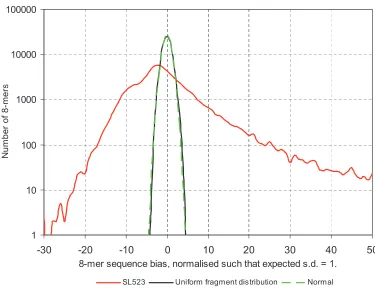
2.3.2 There is a significant sequence-dependent bias in fragment start locations ...50
2.3.3 The bias is consistent within the genome ...53
2.3.4 Sequence bias varies with nucleotide position and experiment ...54
2.3.5 PCMs and model fitting show significant bias differences between experiments †...56
2.3.6 Multiple alternative biases exist within each dataset † ...58
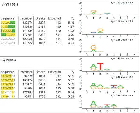
2.3.7 The information from PCMs is consistent with the identity of over-represented 8-mers ‡ ...60
2.3.8 Sequence bias from immunoprecipitated fragments and input DNA is poorly correlated...63
2.3.9 Datasets with different PCMs also show different fragment distributions ...65
2.3.10 Adjustment of fragment distribution for sequence bias ...67
Results ...67
Results: Assessment of improvement ...69
Discussion and conclusion ...70
2.3.11 There is a correlation between sequence bias and 8-mer frequency for some datasets ...71
2.4 Supplementary results ...73
2.4.1 Selecting only a subset of the sequences reduces ‘noise’ from low sequence counts without introducing systematic errors ...73
Introduction ...73
Analysis...74
2.4.2 An offset parameter improves model-fit in single PCM cases ...77
Results: Analysis of GSM418301: HDAC binding control data HeLa cells ...86
Conclusions ...86
2.5 Discussion †...87
2.5.1 ChIP-seq data show an unexpected asymmetric sequence bias around the fragment start position † ...87
2.5.2 ChIP-seq data show an unexpected variety of different sequence bias patterns...88
2.5.3 GC-rich bias arises from GC cleavage preference † ...88
2.5.4 GC-rich fragment ends may propagate through G-quadruplex formation † ...89
2.5.5 Propagation of non GC-rich fragment ends may also involve quadruplex formation †...89
2.5.6 Input data are unsuitable for use as a reference for sequence bias compensation of data from immunoprecipitated fragments ...90
2.5.7 Fragmentation in GC-rich sequence may be associated with CG dinucleotide underrepresentation in the genome ...91
2.5.8 Fragmentation in GC-rich sequences provide a possible explanation for poor qualityArabidopsisChIP-seq data ...92
Chapter 3 Sequence bias in RNA-seq experiments...94
3.1 Introduction ...94
3.2 Method ...95
3.2.1 Data sources ‡ ...95
Mus musculusfrom the Wold lab...95
Homo sapiens GSM484895...95
Arabidopsis thaliana mRNA...96
Homo sapiensERA00183 using the FRT protocol...96
3.2.2 Fragment alignment ...96
3.2.3 Analysis of RNA fragment start sites †...97
3.3 Results ...98
3.3.1 Modelling RNA fragmentation identifies regions with different bias characteristics ‡...98
3.3.2 The PCMs for the 5’ and 3’ ends of RNA-seq fragments are very similar ...103
3.3.3 No over-fitting seen with RNA-seq data using up to nine PCMs ‡ ...103
3.3.4 RNA-seq data processed using the FRT-seq protocol ‡ ...105
3.4 Discussion...108
3.4.1 Two distinct bias regions in RNA-seq data indicate two distinct molecular mechanisms † ...108
3.4.2 Random hexamer related RNA-seq bias in nucleotides 1-6 †...108
3.4.3 Reverse-transcriptase related bias from nucleotide seven onwards † ...109
3.4.4 Implications for correcting bias in RNA-seq † ...109
Chapter 4 Protein binding site fingerprints in ChIP-seq data...110
4.2.2 Identification of over-represented motifs...113
4.2.3 Identification of motif matches in the vicinity of peaks ...113
4.2.4 Calculation of fragment start fingerprints in the region of motif matches...113
4.2.5 Normalisation of fragment distributions...114
4.3 Results ...115
4.3.1 Peak and motif finding from the NRSF immunoprecipitated SL522 dataset...115
4.3.2 Adjusting for sequence bias makes a significant difference to the binding fingerprint...117
4.3.3 Adjusting for sequence bias improves the alignment between fingerprints from different datasets ...117
4.3.4 The NRSF motif fingerprint adds further support to the principle of correcting for bias ...118
4.3.5 Poorer fingerprint match seen in GABP motifs from different ChIP-seq experiments ...124
4.4 Discussion...124
4.4.1 ChIP-seq data contains information at a single nucleotide resolution ...124
4.4.2 Sloping fingerprints indicate motifs associated with the target protein ...124
4.4.3 Fingerprints may provide more detail as regards protein binding...126
4.4.4 Peaks in binding footprints may provide information on chromatin remodelling by NRSF ...127
4.4.5 Common features in two GABP binding fingerprints may indicate aspects of bond between DNA and GABP ...128
4.4.6 There are significant differences between the two GABP binding fingerprints. ...129
Chapter 5 Using modelling to study SeqA binding in E. coli...131
5.1 Introduction ...131
5.1.1 The role of SeqA in prokaryotic cell replication...131
5.1.2 Applying modelling techniques to ChIP-chip data...132
5.2 Methods ...132
5.2.1 Preparation and choice of ChIP-chip data ...132
5.2.2 Principles of modelling SeqA binding...133
5.2.3 Modelling of the effect of adjacent dinucleotides on SeqA binding...133
5.2.4 Modelling of cooperativity in SeqA binding ...135
5.2.5 Modelling of fragment binding to probe sites ...136
5.2.6 Modelling of global residual parameters ...137
5.2.7 Model fitting ...138
5.3 Results ...140
5.3.1 Regional gain variation...140
5.3.2 Di-nucleotides adjacent to the binding site have a significant effect on binding...141
coli...144
5.4.3 Cooperativity in the binding of SeqA toE. coli...145
Chapter 6 Conclusions and further work...147
6.1 The use of modelling to extract additional information from genomic data ...147
6.1.1 Conclusions...147
6.1.2 Further work ...148
6.2 Sequence bias in next generation sequencing data...149
6.2.1 Conclusions...149
6.2.2 Further work ...149
6.3 Obtaining information about protein binding from ChIP-chip data...150
6.3.1 Conclusions...150
6.3.2 Further work ...150
6.4 Obtaining information about protein binding from ChIP-seq data ...150
6.4.1 Conclusions...150
6.4.2 Further work ...151
Appendix A A Method for locating non-unique regions in genomes... 152
A-1 Introduction...152
A-2 Method...154
A-3 Results...159
A-4 Discussion, conclusions and further work ...160
Appendix B Additional nucleotide bias results ‡ ... 162
Appendix C Additional ChIP-seq model-fitting results ... 169
C-1 Early Myers/HudsonAlpha lab results ‡ ...169
C-2 A second pair of technical replicates with contrasting characteristics ‡ ...169
C-3 Late Myers/HudsonAlpha lab results ‡ ...171
C-4 Yale/UC-Davis/Harvard lab ChIP-seq data ‡ ...172
C-5 Cheung et al ‡ ...175
C-6 Arabidopsis dataset...177
Appendix D Additional RNA-seq model-fitting results ‡... 178
Appendix E Software architecture... 181
E-1 General principles ...181
E-2 Software architecture ...182
Appendix F Ancillary algorithms ... 184
F-1 Assessing significance using Pearson’s coefficient and the Fisher transformation...184
F-2 Calculation of cumulative normal values for large z...184
G-3 Dynamic distribution of SeqA protein across the chromosome of Escherichia coli K-12 ..188 G-4 Variable structure motifs for transcription factor binding sites ...189
Bibliography ... 190
† indicates that the section is substantially identical to a section of the paper to be submitted to NAR. ‡ indicates that the section or appendix is substantially identical to a section in the supplementary data
2-1 Over- and underrepresented sequences show significant sequence bias. ...51
2-2 All fragments associated with the TGGAATGG 8-mer from two datasets. ...62
2-3 Compensation using sequence bias predicted from the model yields most improvement in signal to noise ratio...70
2-4 Pearson coefficients indicate equivalence of PCMs generated with different threshold values. ...77
3-1 Pearson correlation coefficient indicating the fit between model and data for two different models...101
A-1 Data requirements for each entry in the hash table ...157
List of figures
1-1 Example ChIP-seq data. ...11-2 Examples of laboratory sonicators. ...8
1-3 Processing and amplification of DNA fragments for use in the Illumina sequencer. ...10
1-4 Amplification and sequencing of fragments on the flow cell. ...13
1-5 Definition of fragment start and end. ...15
1-6 Examples of artefacts where peaks are seen in both input and immunoprecipitated tags...16
1-7 RNA fragment is converted to a slightly shorter double stranded DNA fragment during reverse transcription...21
2-1 Relationship between the probability of DNA fragmenting and the local DNA sequence...33
2-2 Simple demonstration of the derivation ofYs. ...34
2-3 Distribution of Ys shows a log normal characteristic...35
2-4 Distribution of mutual information for the sequence sets associated with each nucleotide shows a log normal characteristic. ...40
2-5 Representation of core Nelder-Mead optimisation step...46
2-6 An example of the use of ‘Zoom’ when displaying logos. ...48
2-7 Fragment ends for two primary datasets have similar distributions...50
2-8 Sequence bias distribution for SL523 is significantly different from that of a uniform fragment distribution...53
2-9 Consistency of strong sequence bias within the genome. ...54
2-10 The bias of individual nucleotide positions is significantly different from that of uniformly distributed fragments...55
2-11 SL117 and SL523 PCMs show very different sequence biases. ...56
2-12 ChIP-seq sequence bias PCMs with sequence biases predominantly within the fragment ...59
2-16 Sequence bias of immunoprecipitated DNA is poorly correlated with the input DNA
sequence bias. ...65
2-17 Similarity of rolling average of tag distribution at binding peaks contrasts with significant differences in underlying tag distribution...66
2-18 Correction for sequence bias reduces some of the noise in ChIP-seq peaks. ...68
2-19 Averaging can be used to give an indication of the underlying fragmentation pattern if the DNA sequence does not influence fragmentation...69
2-20 In some experiments there is a correlation between the number of 8-mers in the genome and sequence bias. ...72
2-21 C. elegansshows a different relationship between sequence bias 8-mer population and sequence bias than that which is shown byH. sapiensdata...73
2-22 Variation of bias correlation with threshold ...74
2-23 Comparison of SL523 PCMs generated by thresholds set to 5000 and 50000...76
2-24 Model fitting of SM217 data improved through the use of an offset parameter...78
2-25 Variation of BIC and Pearson coefficient with the number of PCMs...81
2-26 Cross validation shows no over fitting with up to 15 PCMs ...82
2-27 The effect of adding extra PCMs differs between experiments ...83
2-28 Extract from Figure 1 of Schwartz et al. ...85
2-29 Sequence bias for GSM393947 shows additional features not identified by Schwartz et al...85
2-30 Analysis of region sequence bias in GSM418301. ...86
2-31 ChIP-seq fragment distribution in Arabidopsis. ...93
3-1 The output of a model with no sequence dependency still shows a small degree of correlation with the experimental data. ...99
3-2 Four PCMs showing sequence bias for the first 14 nucleotides of RNA-seq fragments. ...100
3-3 Four PCMs generated to match the first six nucleotides at the start of RNA-seq fragments, and a single PCMs cover the nucleotides from position seven onwards...101
3-4 No evidence of over-fitting in regions not used for model fitting. ...102
3-5 No over-fitting seen for up to nine PCMs. ...104
3-6 Nine PCMs obtained from model-fitting SRX000352 RNA-seq data. ...104
3-7 The results of single PCM model-fitting and from creating an ‘average’ of multiple PCM model fitting are very similar. ...105
3-8 Model fitting of FRT-seq data 5’ fragment end...106
3-9 A region FRT-seq data from the 5’ fragment end showing poor matching between observed data and model...106
3-10 Model fitting of FRT-seq data 3’ fragment end...107
4-1 Relationship of fragment starts to motif...111
4-2 Example peak from the SL522 dataset. ...116
4-3 Ten Overrepresented motifs from the top 1000 peaks in the SL522 dataset. ...116
two datasets show very different patterns...121
4-7 NRSF fingerprints from different datasets are similar after sequence bias compensation...122
4-8 GABP fingerprints from different datasets show some similarity, but also significant differences...123
4-9 Origin of slopes in fingerprints for target proteins. ...126
4-10 Fragment start fingerprint for GABP motif and SL610 dataset ...128
4-11 Over-represented dual GABP binding motif found in binding peaks of SL223 dataset. ...129
5-1 Section of genome showing core SeqA consensus motif and flanking dinucleotide sequences. ...134
5-2 GATC motif and two adjacent motifs...135
5-3 Mapping from binding sites to probe sites...137
5-4 Two regions of theE. coligenome comparing the observed (red) and model (green)...139
5-5 Regional gain variation in SeqA binding. ...141
5-6 Effect of adjacent dinucleotides on SeqA binding...141
5-7 Comparison of cooperative binding found by model fitting in each third genome. ...142
5-8 Effect of GATC site spacing on GATC binding obtained using constructed oligonucleotides...146
A-1 Sequence alignment using the hash table. ...156
A-2 Comparison of published ChIP-seq data and unmappability. ...159
A-3 Comparison of published ChIP-seq data and unmappability. ...160
B-1 Two technical replicates SL117 and SL523 show very different characteristics. ...163
B-2 Four early datasets from the Myers/HudsonAlpha lab show similar characteristics...164
B-3 Later Myers/HudsonAlpha results differ significantly from early results. ...165
B-4 Data from the Snyder/Yale lab show a variety of different characteristics...166
B-5 Log mutual information distribution for Y1109-1 shows a complex picture underlies the simple interaction intensity and spread values ...167
B-6 A second example showing similarity between coincident technical replicates and differences between replicates from different dates. ...167
B-7 Input fragments fromC. elegansChIP-seq experiments ...168
B-8 Input fragments from anArabidopsisChIP-seq experiments ...168
C-1 Two early datasets from the Myers/HudsonAlpha lab. ...169
C-2 Four input technical replicates from the same cell line with a significant range in sequence bias as indicated by the variety of PCMs ...170
C-3 Two later datasets from the Myers/HudsonAlpha lab showing a variety of multi-PCM characteristics. ...171
C-4 Two sets of experimental data from the Yale/UC-Davis/Harvard lab which show CG bias around the fragment start side...172
C-5 Four sets of Yale/UC-Davis/Harvard data which show strong A/T bias only in the nucleotides within the fragment...173
C-9 Nucleotide bias characteristics from one sample ofArabidopsisinput data...177
D-1 RNA-seq model-fitting: GSM484895 5’ end (Homo sapiens) ...178
D-2 RNA-seq model-fitting: Mouse skeletal data - Wold lab (SRX000352)...179
D-3 RNA-seq model-fitting: Mouse brain- Wold lab (SRX001866) ...179
D-4 RNA-seq model-fitting: Arabidopsis 24 hr: Replicate 1...180
D-5 RNA-seq model-fitting: Arabidopsis 24 hr: Replicate 2...180
E-1 Interactions between program modules. ...183
G-1 Spacing of adjacent GATC motifs ...188
I would like to thank the following people:
My wifeJenny, without whose support and encouragement this PhD would not have been possible;
My supervisors,Dr Sascha OttandProfessor Jim Beynon;
My childrenNaomi and Jacobwho encouraged me by regarding it as cool that their dad was doing a PhD in genetics;
The members of my PhD advisory board:Professor Richard Napier,Dr Andrew
Mead and Dr Isabelle Carre; for their interest in what I have been doing, and
their support and advice;
My PhD examiners for their care and attention to detail in reviewing the thesis and for their extensive and extremely helpful comments;
Emma Cooke and Dr. Katherine Denby for kindly providing the Arabidopsis
RNA-seq data that are analysed in this thesis;
Dr. Sally Adams for kindly providing the Arabidopsis LHY ChIP-seq data that
are analysed in this thesis;
The members of Sascha Ott’s group as they have come and gone over the three years of the PhD, with particular thanks toBoris Noyvert andLaura Baxter, for their many helpful comments and suggestions;
Other members of the Systems Biology group at Warwick for their helpful support during this work; in particular thanks to Jay Moore and Siren Veflingstad;
All of the staff at MOAC for their support and encouragement;
Professor Alison Rodger for her support, encouragement, advice and friendship during my time as a student in MOAC;
The creators of the cisGenome tool which has proved to be an invaluable foundation for much of the work described in this thesis;
This thesis is presented in accordance with the regulations for the degree of Doctor of Philosophy. No part of this work has been previously submitted for another degree. At the time of submission of this thesis, some sections of this work were in the process of being submitted for publication. These sections are indicated by the symbols † and ‡ in the headings. Appendix G provides details of papers that were published during the preparation of the PhD for which I was a co-author. These are peripheral to the main thesis. My contribution to these papers and the relationship of this work to the thesis are identified in Appendix G.
Many high throughput sequencing protocols for RNA and DNA require that the polynucleic acid is fragmented so that the identity of a limited number of nucleic acids of one or both of the ends of the fragments can be determined by sequencing. The nucleic acid sequence allows the fragment to be located within the genome, and the fragment distribution can then be used for a variety of different purposes. In the case of DNA this includes identifying the locations where specific proteins are bound to the genome. In the case of RNA this includes quantifying the expression levels of different gene variants or transcripts. If the locations of the polynucleic acid fragments are partly determined by the underlying nucleic acid sequence this could bias any results derived from the data. Unfortunately, such sequence dependencies have already been observed in the distribution of both RNA and DNA fragments. Previous analyses of such data in order to reduce the bias have examined the role of regional characteristics such as GC bias, or the bias towards a specific sequence at the start of the fragments.
This thesis introduces a new method for modelling the bias which considers the degree to which the nucleotide sequence affects the likelihood of a fragment originating at that location. This shows that there is often not a single bias characteristic, but multiple, alternative sequence biases that coexist within a single dataset. This also shows that the nucleotide sequence immediately proximal to the fragment also has a significant effect on the fragment likelihood. This new approach highlights characteristics that were previously hidden and provides a more powerful basis for correcting such bias.
Multiple alternative sequence biases are observed when both RNA and DNA are fragmented, but the more detailed information provided by the new technique shows in detail how the characteristics are different for RNA and DNA and indicates that very different molecular mechanisms are responsible for the biases in the two processes.
This thesis also shows how removing the effect of this bias in ChIP-seq experiments can reveal more subtle features of the distribution of the fragments. This can provide information on the nature of the binding between proteins and the DNA with per-nucleotide precision, revealed through the change in likelihood of the DNA fragmenting at each position in the binding site.
3D Three Dimensional
DNA Deoxyribonucleic Acid
CD4 Cluster of Differentiation 4: A glycoprotein expressed on the surface of
certain cells
cDNA complementary DNA: DNA that has been synthesized from messenger
RNA
CPU Central Processing Unit
EM Expectation Maximization
ENCODE Encyclopaedia of DNA Elements
EPSRC Engineering and Physical Sciences Research Council
GABP Growth-associated Binding Protein
GEO Gene Expression Omnibus
GUI Graphical User Interface
IP Immunoprecipitated
MEME Multiple Expectation Maximization for Motif Elicitation
NCBI National Centre for Biotechnology Information
mRNA Messenger RNA
NAR Nucleic Acids Research
NRSF Neuron-restrictive Silencer Factor
oriC Origin of chromosomal replication
PCAF P300/CBP-Associated Factor: A transcription factor
PCR Polymerase Chain Reaction
PSSM Position Specific Scoring Matrix
PCM Position Coefficient Matrix
QuEST Quantitative Enrichment of Sequence Tags
RNA Ribonucleic Acid
SRA Sequence Read Archive
SNP Single Nucleotide Polymorphisms
Glossary
ChIP-chip Chromatin Immunoprecipitation followed by DNA quantification using
microarray technology (chip) which is used to determine protein binding to DNA
ChIP-seq Chromatin Immunoprecipitation followed by sequencing, which is used to
determine protein binding to DNA.
CD4 cells A type of lymphocyte (white blood cell) cell with a CD4 receptor,
HeLa A common immortal human cell line derived from a cancer cell line taken from
Henrietta Lacks.
K562 An immortalised human cell line created from myelogenous leukaemia cells.
Chapter 1
Introduction
1.1 Motivation and overview
A way of introducing the motivation for the work described in this thesis is by reference to the graphs shown in Figure 1-1. These show the results from a ChIP-seq experiment whose purpose was to identify the locations in the genome where specific proteins were bound. During ChIP-seq experiments DNA is extracted from cells, fragmented, and the ends of the fragments are sequenced, generating the sequence ‘tags’ which are used to identify from where in the genome they came.
Figure 1-1 is a histogram of the data for a short region of the genome, with each bar indicating the number of fragments that were found to start (upper graph) or finish (lower graph) with respect to the forward strand direction at each genomic coordinate. In such experiments the data are then used to identify the regions where the target protein was originally bound. Various techniques and algorithms have been developed to identify these regions using the data but at the heart of all of the algorithms some form of averaging is applied to the data to remove what appears to be noise in the data and so create a smoothed or averaged version of the distributions. The various algorithms then use the smoothed data to determine the likely locations where the proteins were bound.
Figure 1-1 Example ChIP-seq data. a) The distribution of fragment starts with respect to the
direction of the forward strand in a region of the genome. b) Distribution of fragment ends. Each bar indicates the number of fragments associated with a single genomic coordinate.
The motivation for the research described in this thesis was a growing suspicion that by averaging the data in this way, information was being discarded that could otherwise have been used to provide more details about the binding of proteins to the DNA. The initial
a)
suspicion that this was the case arose because of apparent similarities in the data from the same region in similar experiments. This implied a degree of correlation in the relationship between fragment start position and local sequence and suggested that the sequence tags contained information at the level of individual nucleotides, and therefore the seemingly random variation in the fragment counts in Figure 1-1 is not simply noise.
This led to a number of interrelated avenues of research, each of which is covered in separate chapters within this thesis. These avenues confirmed that there is additional information that can be obtained from the fragment distribution and that this can shed light on a number of aspects of both ChIP-seq and RNA-seq experiments. In order to analyse these effects, tools were developed based on model fitting. This approach was then found to have the potential for wider application in interpreting the results of ChIP-chip experiments. The tools and some results from analysing ChIP-chip experiments are also described.
1.2 Overview of the document structure
The core of this thesis consists of six chapters, starting with this first introductory chapter which provides the background to the work described in the thesis and proceeding through to a concluding chapter which draws the various threads together. Between the two are a series of four relatively self contained chapters describing various aspects of the work that has been carried out, each of which has an ‘introduction, results, discussion’ format that deals with the specific topic. In some cases there is a short discussion section directly associated with specific results. This is done when the discussion is largely unrelated to the rest of the chapter, or provides key ideas that form the basis of work that is described in the following results sections.
1.2.1 Relationship to published papers
The information presented in Chapters 2 and 3 has also been covered in an article together with extensive supplementary data that has been submitted to Nucleic Acids Research (NAR). Those sections of the thesis that align closely to text in the paper itself are marked †, and those sections of the text that align with text in the supplementary data for this paper are marked ‡.
1.2.2 Appendices
information was required in order to carry out the analysis in Chapter 2, although the details of how this was carried out are not relevant to the main body of the thesis. This work was carried out because at the time this information was required there was no generally available tool for doing this.
Appendix B and C are supplementary material for Chapter 2, providing more analysis of ChIP-seq data to support the analysis within this chapter. Appendix D is supplementary material for Chapter 3 and provides an analysis of more RNA-seq data to support this chapter.
Appendix E provides a general introduction to the software methodologies and architecture that were used during the work described in this thesis. Appendix F is referenced at various points in the thesis and provides supporting information for some of the algorithms and mathematical analysis that were used. Finally, Appendix G provides a brief summary of the contributions by the author to various journal publications that were prepared during the research described in this thesis, and describes the relationship between the contribution to the papers and the thesis.
1.3 Background
For many centuries, one of the core mysteries in the study of living organisms was the mechanism by which the information that determined the nature of an organism was passed from one generation to the next, and how the information was then used to control the growth and functioning of each successive generation of organisms. The foundation for the solution to this mystery was laid in the 1660s when Robert Hooke was first able to show that living organisms were composed of very large numbers of minute cells, sharing many features in common but nevertheless capable of being tailored to carry out the many different roles required in even the most basic of multicellular organisms [41].
While this laid the foundation, it also demonstrated the challenge faced by anyone attempting to solve this mystery, in that Hooke’s observations and later interpretations of these observations showed that the information that was being sought was wholly contained within these microscopic cells.
show that the information relating to individual characteristics was consistently contained within specific chromosomes.
At about the same time, the rules of inheritance were being determined through observations of the variation in the characteristics of an individual from one generation to the next within a species. This lead to the idea of well defined units of inherited information, for which the term gene was introduced in 1909 by Wilhelm Johannsen [48].
The solution to the problem of how the abstract genetic information that is associated with the gene was connected to the physical structure of the cell came in 1941 with the concept of “one-gene-one-enzyme” where it was proposed that each of the different enzymes in the cell was associated with a one unit of genetic inheritance [10]. It has been observed that this finally began to connect genetics, which had previously been a specialised science with its own language and ideas, to the rest of the biological sciences [43].
The pivotal insight that showed how the genetic information could be stored and replicated within the chromosomes was the solving of the structure of DNA by Crick and Watson [100, 101]. Subsequently, Crick was able to develop this insight into what he termed the central dogma of molecular biology, the transfer of the genetic information in the DNA to RNA which then determines the sequence of the proteins. This concept is still at the heart of molecular biology [22].
The details of this dogma have continued to be worked out, including the identification of the locations of the genes within the genome to an ever greater precision. This led to the realisation that in eukaryotes, the information that is used to determine the amino acid sequence of the protein is not held in one continuous sequence, but is encoded in a series of short sections or exons, with extended regions or introns in between [11, 12].
The intron-exon structure of genes highlighted one of a growing number of areas where the simple ‘one-gene-one-enzyme’ concept is a simplistic picture of a significantly more complex reality. For example, introns and exons provide the flexibility of being able to select different combinations of exons to create different RNA transcripts in order to produce variants of the protein which can be tailored to different situations where the protein is required [Reviewed in 75].
The advent of high throughput sequencing, which enabled almost the complete DNA sequence of organisms with complex genomes such as Homo sapiensto be determined [56], started to provide answers to this question and significantly, the answer of about 25000 genes was much lower than expected [1]. Furthermore, the significant similarity between many of the genes in different organisms was increasingly showing that the protein coding sequences themselves only contained a small part of the genomic information that determines the structure and function of an organism.
Genes can be considered as being like the instruments of an orchestra which, with essentially the same set of instruments, is capable of playing a vast repertoire of music, from Bach to Bacharach. The structure and character of the music being determined by the order in which the instruments are played, and how they are played.
The same is true of genes. It was increasingly clear that it is the order and degree to which the genes are expressed that is critical, and this is determined by a complex and often subtle network of different interacting components. One of the first aspects of this control network to be examined was the binding of proteins, commonly known as transcription factors, to the region immediately adjacent to the start of the gene where they had a major role in determining when an how much a gene was transcribed into RNA [For a review see 27]. The locations where such proteins bind are commonly referred to as transcription factor binding sites (TFBS). As well as proteins binding to DNA, it became clear that there were many other mechanisms that had a significant role in controlling gene expression. For example, the modification of the DNA itself, often through methylation, also had a role in controlling gene expression, and this was often intimately linked to variation in the structure of the DNA, which is also very important [42, 102]. It was also clear that the RNA, as well as being the intermediate in the transfer of information from DNA to protein sequence, also has a very significant regulatory role with the discovery in 1993 of microRNAs. These are small lengths of RNA that are between 20 and 25 nucleotides in length which are transcribed from many regions of the genome and which then able to control various aspects of the transcription and translation process [59, 80].
At the same time as it was becoming clear that the process of gene regulation was incredibly complex, the continuing development of high throughput sequencers now provided significantly more data from a range of different processes which incorporated sequencing which could be used to help unravel this complexity [53].
protein binding are still poorly understood and high throughput sequencing continues to be widely used to investigate protein binding to DNA. The classic high throughput sequencing process that is used for this is ChIP-seq (Chromatin Immunoprecipitation followed by sequencing) [77]. Another approach, based on microarray technology is ChIP-chip (Chromatin Immunoprecipitation followed by microarray (chip)) procedure. This thesis is concerned with extending the techniques for interpreting the data associated with both of these procedures, so they will both be described in more detail in the following sections.
Next generation sequencing is also widely used to investigate the different RNA transcript variants that are generated from the same gene, using the RNA-seq protocol. This thesis is also concerned with how the extension of the techniques used to interpret ChIP-seq data can also be applied to RNA-seq data, so this process will be introduced in more detail in Section 1.5.
1.4 An introduction to the ChIP-chip and ChIP-seq protocols
Chapter 2 and Chapter 4 both relate in some way to the ChIP-seq procedure [77] whereas chapter 5 relates to the use of the ChIP-chip procedure.
The power and range of these processes have resulted in a vast literature describing these techniques and the results that have been obtained using these techniques. The following is a brief introduction to them, concentrating on some of the aspects of these techniques that are particularly important when considering the results in later sections of this thesis.
1.4.1 The motivation for studying protein binding to DNA
As well as using this information to try and understand gene regulatory networks in different species these techniques have also been used to ascertain the extent of the variation between individuals in a species in order to understand how this variation might explain the specific characteristics of the individuals [e.g. 50].
Gene regulation is a very dynamic process, and both ChIP-chip and ChIP-seq are used to measure the variation in time of protein binding to the DNA in order to understand how the changes are linked to changes in response to external stimuli [e.g. 61], or other signalling pathways [e.g 29], or changes over time as a result of clock networks within living organisms [e.g. 19]. The changes in protein binding can also be associated with changes in gene expression as part of the process of identifying the myriad of different signalling pathways within cells.
As well as proteins playing a role in gene regulation, there is a growing awareness of the role of the chromatin structure in gene regulation, and the use of ChIP-seq and ChIP-chip protocols to locate where structural proteins such as histones bind to the DNA can provide significant information on the chromatin structure [65].
1.4.2 Preparing the DNA for ChIP-seq and ChIP-chip: protein fixing with formaldehyde
In both ChIP-seq and ChIP-chip processes the DNA has to be extracted and purified from the cell while the proteins are still bound to the DNA in order that their presence can be used to identify the protein binding sites. In order to ensure that the proteins remain bound, one of the first stages in the protocol is to fix the proteins to the DNA using formaldehyde.
1.4.3 DNA extraction and fragmentation
Following DNA extraction from the cell, the DNA is then fragmented into lengths that are of the order 100 to 300 base-pairs, typically using sonication. This is perhaps the least well controlled of the stages in the process because of the difficulty of applying the same amount of sonication to the sample in successive experiments, and the difficulty in ensuring that all of the sample is equally affected by the sonication.
Sonication is a well established process for disrupting biological material such as cells, and there are a number of types of standard laboratory sonicators that have been used for many years. There are a variety of different approaches to the problem of applying ultrasound to the samples, including placing a tip which is vibrated at ultrasonic frequencies into the sample or placing multiple samples into a water-bath that is then excited with ultrasonic vibrations which are carried through the water to the sample (Figure 1-2).
Figure 1-2 Examples of laboratory sonicators. a) Tip based sonicator where a tip is placed into
the liquid to be sonicated (www.sonics.com) b) The Bioruptor® (www.diagenode.com). An example of systems where multiple samples are sealed in individual tubes and immersed in a water bath through which the ultrasound is carried to the samples.
Products such as the Bioruptor® from Diagenode have been designed specifically for the task of fragmenting DNA samples, and are designed to try and ensure that the ultrasound is evenly distributed through all of the samples, and that the samples are kept cool.
to minimise this by using short bursts of ultrasound interspersed with cooling on ice, or by actively cooling the water in water-bath based sonicators.
It is generally understood that DNA fragmentation occurs as a result of cavitation that occurs within the sample [69, 93]. Microscopic bubbles form and grow within the solution during the negative pressure half-cycle of the pressure wave, and in the positive half cycle they reduce in size. If they grow beyond a certain critical size then they collapse catastrophically resulting in a very intense localised release of energy. DNA fragmentation is believed to occur largely as a result of local shear stresses that occur when the bubbles collapse, although the effect of localised heating may also be significant as temperatures can briefly reach 5000 ºC [93].
Bubble collapse also produces free radicals, and it has been suggested that these may also play a role in fragmenting the DNA. It is thought that such free radicals will cleave the DNA at random locations whereas cleavage resulting from shear stresses is likely to reduce the DNA fragment size by a progressive series of halvings [35].
It is known that the cavitation that occurs during sonication is dependent on the dissolved gases in the solution [71] which may explain why it has been observed that the degree of fragmentation that can be achieved can be a function of the dissolved gases that are present in the sample [28].
The sonication typically produces fragments over a wide range of lengths, but many DNA sequencing or microarray technologies perform best with fragments that cover a relatively narrow range of lengths. It is therefore necessary to tune the sonication process so that the peak in the distribution of fragment lengths that are obtained is roughly in the region preferred by the subsequent stages of the process, which is typically of the order of 200 to 400 basepairs.
1.4.4 Immunoprecipitation and size selection
In order that the fragments can ultimately be sequenced, it is necessary to ligate adaptors onto the end of the fragments such that the adaptors at each end of each single stranded fragment have different sequences and are not simply complements of each other. If a double stranded adaptor was ligated onto the ends of the fragments then the adaptors at each end of the single stranded DNA would be complements of each other. In the case of the Illumina protocol, the use of Y adaptors, which are double stranded for part of their length and single stranded for the rest, ensures that, after amplification, the adaptors at each end of the fragment have different sequences.
a)
b)
c)
d)
e)
f)
g)
[image:27.595.89.534.256.517.2]A
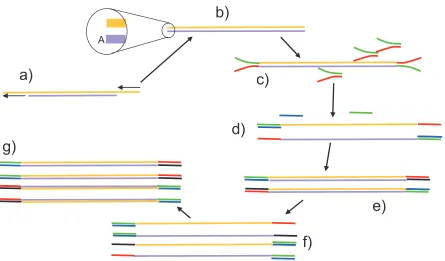
Figure 1-3 Processing and amplification of DNA fragments for use in the Illumina sequencer.
a) Double stranded DNA fragments are repaired by extending 3’ excessive ends and digesting 3’ protruding ends. b) Blunt ended strands to which an A overhang is added to the 3’ end of each strand. c) This allows a ‘Y’ adaptor to be ligated onto both ends which starts with a short section of double stranded DNA and continues with two sections of uncomplementary single stranded DNA. d) These are denatured and then allowed to bind to two added primers (green and blue), although at this stage only one of them is able to bind to the single stranded adaptor sequences. e) The second DNA strands are synthesised. f) The strands are denatured, and at this stage both primers are able to bind to the end adaptor sequences. g) The process continues, creating a large number of identical fragments with different adaptor sequences at each end.
the adaptor sequence at each end of the fragments after amplification are different. In the figure a green and red adaptor, with different nucleotide sequences, end up on either end of one of the strands of the DNA, and their complementary red and blue adaptors on the ends of the other strand.
When the fragments are amplified for the ChIP-chip process a conventional fully double stranded adaptor is used as there is no requirement for the adaptors at either end to have different sequences.
As well as amplification the fragments are size selected, where the DNA is run on an agarose gel and a strip of gel is excised that corresponds to the optimal range of DNA lengths. The end of the process yields a sample of fragments at an adequate concentration for quantification using either microarray (ChIP-chip) or sequencing (ChIP-chip) technologies.
1.4.5 The use of input DNA or mock precipitated DNA as a control
The purpose of ChIP-seq and ChIP-chip is to use the distribution of the immunoprecipitated DNA within the genome to locate positions where proteins bind to the DNA and also assess the degree of binding, which is done by looking at the locations and sizes of the peaks in the distribution.
Unfortunately, there are frequently peaks in the distribution of the immunoprecipitated DNA that do not correspond to protein binding locations but are instead artefacts that arise out of the bio-chemistry of the process and also the bioinformatics of the alignment process. One of the ways of demonstrating that these are artefacts is to examine the fragment distribution in a control which does not involve the immunoprecipitation of DNA fragments attached to the target protein. If the peaks are also present in the control then their presence in the immunoprecipitated fragments is assumed to be as a result of an artefact in the process and the peaks are ignored [52]. There are two ways in which a control can be generated for such experiments [77 p 672].
A second approach that has been adopted in order to avoid the problems of low sample quantities from mock immunoprecipitation is to use a sample of the input DNA as a control, as it has been shown that many of the artefacts also show up as peaks in the input DNA, providing the information needed to remove the artefacts in the sample
In either case, it is common practise not to process a control that is associated with every set of immunoprecipitated fragments, but instead to produce a control for a particular cell line that has been treated in a particular way, and use it as the control for a large number of experiments that have been done with the same cell line and treatment. This is done on the assumptions that there is not a significant variation in the distribution that is seen between controls and that the artefacts that are seen are common to all the controls and so it is not necessary to produce a separate control for each experiment.
1.4.6 Fragment quantification using ChIP-chip
ChIP-chip is the earliest of the two technologies and uses microarrays to quantify the amount of DNA from different regions of the genome [63]. Microarrays are small glass slides that have been spotted with 100’s of thousands of individual spots, each containing thousands of identical copies of a short sequence of single stranded DNA, typically between 30 and 50 nucleotides long. Each spot contains DNA with a different sequence, and each will match a specific location within the genome. When the sample is washed over the array, fragments whose sequence matches the sequence of the DNA on a specific spot will bind, and the overall quantity bound at any spot can be measured using fluorescence.
a)
b) c) d)
e) g)
f)
h)
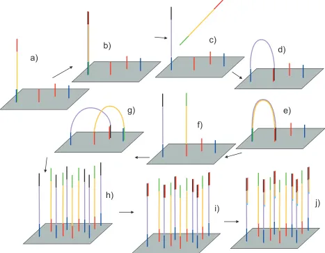
[image:30.595.86.553.73.436.2]i) j)
Figure 1-4 Amplification and sequencing of fragments on the flow cell. a) After amplification
1.4.7 Fragment identification and quantification using ChIP-seq
This protocol builds on the experience the ChIP-chip protocol but locates the fragments on the genome using the fast developing, high throughput sequencing technology. This removes the requirement to decide in advance what regions will be sampled and which excluded, and it removes the need to create chips with specific sequences for each organism, and chips for each sampling strategy associated with an organism. There are extensive reviews of both technologies, and comparisons between the two, in the literature [e.g. 30].
In order to locate the source of each fragment within the genome, the end of each fragment is sequenced, resulting in a sequence tag, and the sequence then located within the genome. There are a number of variants of the sequencing protocols that are used to sequence DNA and which can be used within the ChIP-seq process. They do however share many underlying principles. The details of the process employed by the Illumina sequencing platforms are shown in Figure 1-4.
For any given sequence length there will be a certain proportion of sequences that do not map to a unique location in the genome. A number of approaches can be adopted for dealing with such fragments, but the commonest is to disregard them, and chose a sequence length that is sufficient to keep the proportion of disregarded fragments to an acceptably low level. Sequence lengths of 25 or 36 are commonly chosen and have been found to be adequate for sequence alignment to the human genome.
1.4.8 Definition of fragment orientation
Any given sequence tag may align to either the forward strand or the reverse strand of the DNA. The double stranded sequence is molecularly symmetrical, and the choice of which strand is the forward strand was an arbitrary necessity for the purposes of nucleotide numbering. When the fragment is aligned to the genome the convention adopted in this thesis is to define the fragment start and end with respect to the forward strand direction. A sequence tag that aligns to the forward strand thus identifies a fragment start, and a tag alignment to the reverse strand identifies a fragment end (Figure 1-5a).
sequence is always in a specific orientation with respect to the protein coding sequence, whose direction of transcription can then define the orientation of the sequence.
a) Orientation defined by forward strand
b) Orientation defined by local feature
0 N
Fragment start
Fragment end
Forward strand of chromosome
Fragment
start Fragmentend
Section of chromosome
Figure 1-5 Definition of fragment start and end. Green fragments are shown aligned to a region
of the genome (black) a) Fragment direction defined with respect to the forward strand of a chromosome. b) Direction defined with respect to some local feature such as a nucleotide sequence that matches a specific pattern on a specific strand.
1.4.9 ChIP-seq peak finding algorithms
In the case of ChIP-seq, the fragment location information is then collated. An example of a typical fragment distribution in the region of a transcription factor binding site was shown in Figure 1-1. Various algorithms and their implementations in software have been developed to interpret these data in order to identify the probable locations of the transcription factor binding sites that gave rise to the ChIP-seq results that were obtained [94]. A common factor to all of these algorithms is that they use a smoothed version of the fragment distribution, often by a summation of the counts over a specific window size such as 25 nucleotides. One advantage of such windowing is that it makes the computation more tractable. There is an implicit assumption in doing this that there is no significant information associated with the individual counts, and the nucleotide to nucleotide variation in count is essentially noise that arises out of the fragmentation process..
distributions of the forward reads and the reverse reads such as is used in cisGenome [46] or in the QuEST software [96]. A common feature of many peak finders is that the distribution of the immunoprecipitated fragments is compared to the distribution of the control sample such as the input DNA [47, 85] in order to remove peaks in the data that are as a result of artefacts in the process and not protein binding (Section 1.4.5). These algorithms look for the degree to which the fragments are enriched in some regions as a result of immunoprecipitation compared to the control. They ignore those peaks that are present in the immunoprecipitated DNA because there was a corresponding peak in the input fragment distribution and no enrichment had occurred as a result of immunoprecipitation. Such peaks in the input fragments are as a result of other factors such as the effect of DNA structure on fragmentation or alignment artefacts such as those shown in Figure 1-6.
Bayesian techniques have also been used to interpret the data [91] and other software has been developed to looking specifically for the characteristic shapes of the peaks that indicate a binding site [44]. Examples of such peaks can be seen in Figure 2-17.
Figure 1-6 Examples of artefacts where peaks are seen in both input and
immunoprecipitated tags. a) & c) Peaks in tag distributions of immunoprecipitated DNA where
peaks are also seen the input DNA (b & d). e) Unmappable regions. All plots show a region from chromosome 1 and black indicates forward strand and red the reverse strand. c) & d) are characteristic of artefacts frequently found immediately adjacent to unmappable regions and suggest that fragments from very repetitive regions of the genome that have yet to be sequenced are mapped to other similar slightly less repetitive regions which have been sequenced. They have been mapped because there is only one instance of the specific tag sequence in the sequenced genome.
1.4.10 Motif finding
Once peak finding has been used to identify regions where the target transcription factor was bound, a common task is then to identify the specific locations within these regions
a) IP
b) input
c) IP
d) input
where the protein was bound. One general principle that is frequently adopted is to look for a DNA sequence that is over-represented within these regions compared to the frequency with which it occurs within the overall genome. One improvement that can be made is make the comparison with carefully selected control regions of the genome that are similar in some respect to the region where the peak is located but where was no significant degree of protein binding.
One difficulty that is encountered in motif finding is that transcription factors often do not bind to one specific DNA sequence but instead bind to a range of sequences that are variants of some underlying pattern. The degree of binding is a complex function of the DNA sequence in combination with many other factors such as chromatin conformation and the binding of other proteins nearby on the DNA.
Many algorithms have been developed to try and identify the sequence pattern or motif associated with protein binding. One well established and frequently used algorithm is MEME (Multiple EM for Motif Elicitation) [5]. This built on an early Expectation Maximization (EM) algorithm [58] which assumed that there was a single instance of a variant of the MOTIF in each of the regions and then finds the sets of positions i in the regions j that gives the maximum likelihood that they are the sequences derived from an underlying motif.
The first extension added by MEME was to use sequences from the regions as initial seeds for searching for the underlying motif. Another extension was to remove the assumption that there is only one instance of the sequence in each region. The final extension is that once a motif is found the sites associated with the motif are deemphasised during the search for additional motifs, which improves the ability to find multiple alternative binding motifs.
The motif finding algorithm that is integrated into cisGenome [47] and which is used for motif dinding in this research uses a Gibbs sampling algorithm and a Bayesian approach to identifying conserved motifs within the regions of the ChIP-seq peaks [45, 64]. In common with MEME, it is able to detect multiple alternative motifs, and also to detect motifs that occur more than once within any one of the set of regions being examined.
1.4.11 Representation of motifs using Position Specific Scoring Matrices (PSSMs)
nucleotides do not correspond to the consensus sequence, and where the motif is better expressed in terms of a tendency towards certain nucleotides at certain positions.
The approach frequently adopted is to represent the motif as a Position Specific Scoring Matrix (PSSM) or Position Weight Matrix (PWM)Psuch that
1,a2 ,c3 ,g ,t
, , ..
, , ,
N i wi wi wi wi
P p p p p
p (1.1)
Each member pi of the ordered setPis a vector of weights wi,nwhich are a measure of the probability of finding the nucleotide n at position i. These can be derived by experimentally identifying locations in the DNA where the protein is known to bind, and counting the number of each of the nucleotides at each of the positions and using the counts as the valueswi,n. If M positions have been identified then
a,c,g,t i n, n
w M
(1.2)It is frequently the case that the values are normalised such that
a,c,g,t ,
1
i n n
w
(1.3)When this is done, then the weights give the likelihood of a nucleotide being found at a particular position if it is known to be a location where the protein binds.
This information can then be used to determine the likelihood of any given nucleotide sequence being associated with a particular motif. For each position in the sequence the likelihood of the nucleotide is compared with the likelihood given the background nucleotide position, and the overall likelihood can then be calculated as the product of the likelihood at each position.
The background distribution that is used can be a simple independent likelihood of each nucleotide, or can be a more complex likelihood, for example based on a third order Markov model of the nucleotide sequence characteristic that is derived for each region of the genome. Such a Markov model is used in motif mapping software such as is found in the cisGenome software suite [46].
1.4.12 The advantages and disadvantages of ChIP-chip
ChIP-chip and ChIP-seq are both widely used technologies for determining the level of protein binding to DNA. ChIP-chip is the earliest of the technologies and is still the cheapest and offers the possibility of having results in a matter of days. Its disadvantage is that it is essentially an analogue technology which limits the precision of the measurements, and the results are spatially quantised along the genome, as set by the spacing along the genome of the probes that are used to bind to the DNA. Consequently it only allows the measurement of DNA levels at a specific set of points along the genome. The more recent ChIP-seq process [77], building on the capabilities of high throughput sequencing technologies, has the advantage that it has a greater dynamic range, being able to measure differential protein binding over many orders of magnitude, and can also provide very detailed binding information, down to the level of individual nucleotide positions (Chapter 4). It is nevertheless the case that it is relatively expensive and has a long turnaround time from starting the experiment to obtaining final results.
1.4.13 The use of sonication to explore chromatin structure
There has already been some recognition that the locations where DNA breaks during the sonication stage of the ChIP-seq protocol are not uniformly distributed, and can in themselves be used to investigate genomic characteristics. It has been found [3, 95] that fragments send to occur preferentially in the regions where the chromatin is more open, such as is the case in active promoter regions. These investigations also showed that the degree to which the fragments were able to identify the open regions of the chromatin was dependent on the size of the fragment that was selected after sonication, with the shorter fragments being better indicators of open chromatin [3].
1.5 An introduction to the RNA-seq protocol
The use of high throughput sequencing techniques for analysing RNA data has provided another way in which sequencing can be used to probe the mechanisms within the cell that enable the genetic code to be involved in the control of almost every aspect of the functioning of a cell.
of these microRNAs [31]. The lengths of these RNAs mean that the fragmentation stage that is necessary in DNA sequencing is not required, as each microRNA is short enough to be sequenced in its entirety.
However, the first and still the dominant RNA based protocol is RNA-seq, where the RNA is extracted from the cell, purified and then fragmented so that, by sequencing the ends of the fragments that are obtained, a picture can be constructed of the nucleotide sequence of the RNA molecules that are found in the cell and their relative abundance. The primary purpose of this procedure is to investigate messenger RNA (mRNA) in the cell, where it can be used to investigate the expression levels of genes, and to investigate the different transcript variants [73, 98]. It is then able to be used to refine the genome annotation to provide more detail of the differential transcript expression.
RNA sequencing protocols contain many of the elements from the ChIP-seq like protocols, but there are a number of very specific and important differences. In particular, high throughput sequencing protocols have been designed around the processing and sequencing of DNA, and many of the stages of the procedure such as the amplification using PCR are only currently possible using DNA. Consequently a necessary step in the sequencing of RNA fragments is the conversion of RNA into the complementary DNA sequence using the reverse transcriptase enzyme so that it can then be amplified and sequenced [98]. Reverse transcriptase can only initiate the transcription at a location in the RNA where the complementary strand of DNA is already present which acts as a primer for the process.
The problem that has to be solved when transcribing the RNA fragments to DNA is that the sequences of the fragments are all very different, making it difficult to design a primer or set of primers which will bind to the RNA and act as a primer and allow all of the fragments to be converted to DNA in an unbiased way.
The solution that has been widely adopted is to create a set of DNA primers that are six nucleotides long and are a random mix of the 4096 different combinations of six nucleotides that are present in such hexamers [32]1. A six nucleotide length primer is sufficiently long to enable reverse transcriptase to bind and start the reverse transcription process, and there will be a hexamer present in the mix that can bind to any position in an RNA fragment.
1The primary subject of this journal article was the hypomethylation of cancer genes. However this article now
Random DNA Hexamer
a) T T A A T G G G C A A A
RNA
5' A C G G G A A U U A C G G A A U U A C C C G U U U C G 3'
b)
C C T T A A T G A A T G G G C A A A 5'
RNA
5' A C G G G A A U U A C G G A A U U A C C C G U U U C G 3'
c) DNA
3' T G C C C T T A A T G C C T T A A T G G G C A A A RNA
5' A C G G G A A U U A C G G A A U U A C C C G U U U C G 3'
d) DNA
3' T G C C C T T A A T G C C T T A A T G G G C A A A 5'
C G G G A A Random DNA Hexamer
e) DNA
3' T G C C C T T A A T G C C T T A A T G G G C A A A 5'
5' C G G G A A T T
f) Double stranded DNA
3' T G C C C T T A A T G C C T T A A T G G G C A A A 5'
5' C G G G A A T T A C C C G T T T A C C C G T T T 3'
g) Overhangs removed
3' G C C C T T A A T G C C T T A A T G G G C A A A 5'
5' C G G G A A T T A C C C G T T T A C C C G T T T 3'
[image:38.595.78.535.70.585.2]DNA Polymerase Reverse transcriptase
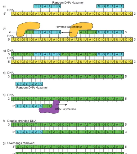
Figure 1-7 RNA fragment is converted to a slightly shorter double stranded DNA fragment
during reverse transcription. a) Random DNA hexamers binds to RNA. b) Reverse transcriptase
The conversion is a two stage process. In the first stage, complementary DNA is added to the single stranded RNA fragments in order to create a double stranded polynucleotide that is a pairing of DNA and RNA. These are then separated, and the single stranded DNA converted to double stranded DNA using DNA polymerase (Figure 1-7).
Both of these processes require a DNA primer to be bound to the DNA or RNA to allow the enzyme to bind and reverse transcription or polymerisation to proceed. In both cases the primers will bind at multiple locations, and the transcription will proceed at each location until the enzyme meets the location of the next primer. At this point the enzyme can complete the second strand right up to the primer. In both cases however, transcription can only start from the position where the first primer bound, and this may not be right at the start of the template RNA or DNA fragment. A consequence of this is that the ends of the final DNA fragment that is sequenced will not correspond to the ends of the fragment that was originally formed when the RNA was fragmented.
1.6 Introduction to the thesis
One feature of the use of next generation sequencing in the ChIP-seq protocol is that while each experiment generates very large quantities of data, much of this is discarded during the processing of the data to identify protein binding sites.
The area of research that was the original motivation for the work described in this thesis was a suspicion that within this discarded data there were data that could be used to provide more information about the nature of the binding of transcription factors to DNA. The initial investigation centred on the pattern of fragment starts in ChIP-seq data that is associated with over-represented sequences or motifs in the vicinity of peaks in the ChIP-seq data. The initial conclusion is that such patterns can provide an additional source of information about the way that proteins such as transcription factors bind to these sequences. This is covered in Chapter 4.
The reason why this is covered in one of the later chapters of this thesis is that it quickly became clear that there were other genome wide sequence specific effects that influence the probability of the DNA fracturing at any specific location in the genome. It was thought that these effects would need to be analysed further in order to be able to compensate for them if necessary and so get a clearer picture of the way in which proteins that are bound to the DNA might influence DNA fragmentation.
locations. It was clear that fragment starts were associated significantly more frequently with some sequences and less frequently with others. While a degree of sequence dependency has previously been identified, the details, origin and potential impact on the interpretation of results are still poorly understood [25, 26, 88].
This investigation is covered in Chapter 2 which describes a new modelling technique which shows how this sequence dependency is significantly more complex than previously realised. For example, there is a significant variation in this effect between different experiments, which was previously unrecognised. The chapter also describes the mathematical model that was developed to describe the relationship between DNA sequence and the probability of fragmentation at any specific location, and the model fitting algorithm that was used to fit the model parameters to the observed data. The more detailed results obtained from this modelling technique allows more informed discussion on the origin and impact of this dependency.
After this model had been developed it was realised that it could also be used to provide a better picture of the sequence bias that occurs in the RNA-seq protocols. This investigation is covered in chapter 3 which mirrors the contents of chapter 2 in that it shows that the effect is significantly more complex than previously acknowledged and that in this complexity can be found information that can help understand the mechanisms that occur during the RNA-seq process.
When the ends of fragments are sequenced in order to align them to the genome, the finite read length means that there will be some sequences where it will not be possible to identify a unique location where the fragment originated in the genome. In this situation the simplest and most commonly adopted practise is to ignore these fragments. This means there will be some regions of the genome where the fragment start density is zero. This is an artefact that needs to be corrected for in order to improve the accuracy of the analysis of sequence dependent fragmentation covered in Chapter 2. At the time of starting this analysis there were no generally available tools for locating the regions in the genome that are unmappable in this way, which is a necessary prerequisite to being able to compensate for this artefact. Consequently an algorithm and associated software was developed that allowed these regions to be identified efficiently. This is described in Appendix A.