Toward spatial impedance estimation for robotic systems

(1)

Toward spatial impedance estimation

for robotic systems

D. (Damiano) Graziosi

MSc Report

Committee:

Dr.ir. D. Dresscher

Dr.ir. N. van der Stap

Dr.ir. P.C. Breedveld

Dr.ir. R.G.K.M. Aarts

September 2018

(2)

(3)

iii

Preface

This thesis concludes my two-year path within the Robotics & Mechatronics department at the University of Twente, leading me to the completion of the MSc program in Systems and Control. Special thanksgivings are due to my university supervisor dr. ir. Douwe Dresscher for his guide, and to the company supervisor dr. ir. Nanda van der Stap for hosting me at TNO and making this collaboration possible.

During this time, I have had the good fortune of encountering people I will always remember, who made this experience truly priceless.

I wholeheartedly thank the university staff for giving me the opportunity to develop myself, and my friends all for making me laugh during those frequent grumpy days.

Finally, I can not refrain from expressing my inmost gratitude to my parents and my brother Matteo for their unconditional presence.

Damiano Graziosi

(4)

(5)

v

Summary

I

n present days, performing complex tasks from a remote site through the use of intermediate mechatronic systems is not an illusion anymore (one can think of the Da Vinci surgical system, for example). That is why telepresence and telemanipulation are topics of research and development within the i-Botics Joint Innovation Center - a collaboration between the University of Twente and TNO. Combining the cognitive ability of the human operator with the robotic capabilities at a distance is the main objective of this cooperation.

Robots never get tired, neither bored nor injured. However, they are still far away from understanding a situation through the senses human beings have been developing for thousand of hundreds of years of evolution on Earth. Therefore, improving these sensing capabilities would allow them to be used even more in complicated tasks where those human abilities and “situational awareness” are required, avoiding human presence in hazardous scenarios (one can think of EOD or pipe inspection robots).

In a typical teleoperated system, unavoidable latencies in between operator (master) and the end-robot (at the slave site) jeopardise transparency (haptic performance) and endanger stability. However, it is known from previous studies that having available a more accurate model of the remote environment, i.e. where the manipulation takes place, would enhance the overall performance the system. For this purpose, an adaptive impedance law can be implemented on each controller side when force/position measurements are available within the Bilateral Impedance Control architecture.

(6)

(7)

vii

1 Introduction

1.1 Problem context 1.1.1 Telemanipulation

T

elemanipulation is considered one of the earliest manifestation of modern robotics(Siciliano and Khatib, 2016); in fact, it can be dated back in the 1940s with the pioneering studies conducted by Goertz (Goertz,1952,1954) in which he presented a system to manipulate radioactive material. At the same time, he coined a terminology that is still commonly accepted: mastersite stands for the local environment (LE) in which the human operator makes decisions while slave indicates the remote environment (RE), where the telecontrolled robot executes the commanded actions.

In its early days, telemanipulation aimed to separate the brain (i.e. whoever plans the task) from the body (i.e. whatever executes it); on the other hand, the latest trend in robotics tends to reconcile these entities by mean of increasing the decision making capability of the robot itself. As noticeable, other terms are used almost interchangeably to indicate telemanipulation, such as telerobotics and teleoperation. While they all share the prefixtele, from the Greek wordτηλ²which means "far off", they put emphasis on different targets: on the object-level manipulation, on the human action of controlling a robot and on the task-level operations, respectively.

However, the commonly accepted goal of these tele-something research is to avoid human beings presence within the RE which, in some cases, might put their safety at risk (e.g. nuclear industry), present scaling factors (dimensions or forces, for example) unobtainable using the solely human body capabilities or be extremely costly to reach (e.g. space applications).

(10)

1.1.2 Environment exploration

For the sake of simplicity, based on the extent of thea prioriknowledge, an operator can face with a:

• totally known RE;

• partially known RE;

• totally unknown RE.

Within each of the above mentioned cases, likewise the tasks to be carried out could be:

• fully determined;

• partially determined;

• totally determined.

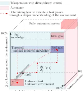
Figure 1.1 sketches the transitions that are needed to determine if and how a task can be carried out: the knowledge about the environment and the duty to tackle are the ordinate and abscissa respectively, while the third axis represent the extent of autonomousness of the mechatronic system.

Determining if and how a task can be executed passes through a minimal knowledge of the environment; i.e. a threshold which depends on the application in hand. For example, if a robot has to grab a glass on a table, awareness about the location of the objects within the 3D space are needed, whereas only a partial recognition of the surrounding area is necessary for that job. When this requisite limit is not yet reached, that is an environment still very unknown, then a further exploration for recognition is needed - upward vertical direction into figure 1.1. Besides, artificial intelligence (AI) techniques together with the dexterous manipulative development of the robots, push this path toward the third dimension in figure 1.1. The ideal goal is represented by a total and thorough knowledge of the remote environment to fully determine how to accomplish the desired task. The latter, as already said, would be fully given only when the real world is known for a reasonable extent: i.e. when the threshold band in figure 1.1 is reached.

This concept can be for example applied to the very hot topic of human-robot interaction (HRI) , where safety is the primary concern: in fact, robots could not safely and "friendly" interact with humans if the boundary conditions (i.e. the RE) are only blurry known.

1.2 Problems description

(11)

CHAPTER 1. INTRODUCTION 3

100%

0%

x: task determination (knowledge-wise) Fully automated system

0%

z:human presenc

e

y:

kno

wledge

ab

out

the

en

vironm

en

t

Teleoperation with direct/shared control Autonomy

[image:11.595.147.415.96.391.2]

through a deeper understanding of the environment Determining how to execute a task passes

Figure 1.1:Environment recognition importance.

back to the operator through an haptic interface can come straight from the sensors (direct force feedback) or computed by the physical engine within the VR; the latter is better known as haptic rendering.

1.2.1 Haptic devices

(12)

1.2.2 Trasparency and stability

As a matter of definition, transparency of an telerobotic system is defined as the fidelity by which the human operator perceives the RE and the naturalness by which he/she can perform the task within the slave site (Tzafestas et al.,2008). In any case, pursuing total transparency should not come at the stake of a stable systems; in fact, in (Hannaford,1989b), the author proved that it exist a trade-off in between stability and performance, measured in this case by the grade of transparency. Later on, in (Franken et al.,2009,2011), the authors proposed a two-layers control architecture to fill the gap in between transparency and passivity by addressing these two properties independently.

1.2.3 Time delay

The communication channel in between the master and the slave allows the data transfer throughout the teleoperation system - defined "barrier" in figure 1.2. Together with foreseeable digital discretization, this information exchange link suffers from unpredictable latencies and low-bandwidth (LF) communications; these questions are even more exacerbated by the supposedly extreme conditions of the operational scenario (one can think to underwater operations, for example). These hurdles make often unpractical to use a direct control in between LE and RE to reflect the interaction forces to the operator, viz. singly position/force controller.

In order to remove this dependency on the time delay introduced by the communication channel, a commonly used alternative is to make the operator interact with an fictitious reproduction (either partially or made completely up) of the remote environment, herein meant as a graphical virtual environment (VE). This situation sees an operator who telemanipulates objects inside a VE which is timely updated -communication channel allowing- upon measured and processed signals from the remote environment. Therefore, through a physics engine (section 2.3), the desired sensory stimuli are transmitted to the user to convey information about a virtual haptic object.

This so built virtual world, constructed upon these new knowledge, would remove the communication latency and data loss dependency which practically always occur in direct telerobotic operations. Potentially, this VE can be seen as a time-delay free middle ground, in which the operator works safely, effectively, inexpensively and rapidly trains specific skills..

1.2.4 Actuatory and sensory capability

(13)

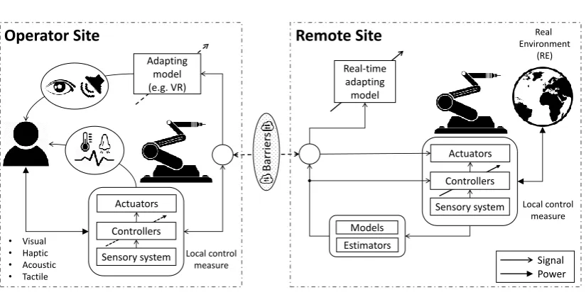
CHAPTER 1. INTRODUCTION 5 Adapting model (e.g. VR) Real-time adapting model Models Estimators Actuators Controllers

Sensory system _Signal

Power Actuators

Controllers

Sensory system

Operator Site

Remote Site

Real

[image:13.595.74.487.116.322.2]

Environment (RE) Local control measure • Visual • Haptic • Acoustic • Tactile Local control measure Barri er s

Figure 1.2:General structure of a teleoperated system.

not be achieved within an open loop operational mode, and this is another reason why haptic rendering1is driving much of today’s haptic virtual environment research, this project included.

1.3 Research goal

Generally speaking, the final goal of every controlled system is to have a complementary sensitivity functionT(s)=UY((ss))=1 within a specific range of frequency. Therefore, promptly knowing the plant behaviour (i.e. its state vector) would allow to generate specific correcting actions to seek that result. In fact, while predictable deviations from the ideal behaviour could be compensated by applying feed-forward, more complex and unforeseen dynamics can only be dealt inside a feedback loop -within the robustness range. In practice, the sensory capability of mechatronic systems could be limited and the state vector x only partially known: that is why estimation theory comes to help engineers to design adaptive controller (e.g. MRAS or STR).

1.3.1 i-Botics

Withini-Botics, the long-terms goal is to automate the environment recognition, along with building a virtual environment in order allow users to perform finer tasks in hazardous environment by means of telerobotic systems. The ultimate goal is to combine visual

1_I.e. _{determining interaction forces with virtual objects when the operator’s motion is measured (for}

(14)

recognition and dynamic identification of the environment to autonomously accomplish otherwise dangerous operations. An example could be inspection/rescue routine tasks; at the same time, the human operator would supervise the mission and fine tunes the details, where needed. A major advantage of this telerobotics approach is that it optimally benefits from combining the cognitive ability of the human operator with the robotic capabilities at a distance.

1.3.2 Research questions

Referring to section 1.2, this research investigates possible relives to the latency issue which, in turn, would result in improved performance, the transparency in particular. Specifically, plenty of studies advocated that an upfront (ideally) or online knowledge about the nature of the real environment would lead to such an enhanced telepresence. However, the validation of this claims come from simplistic case studies in which ad-hoc experimental setups have been employed, and the environment has the dimension of a point. Based on these premises, the following research questions have be formulated:

How can a punctual estimation of the dynamic properties of the environment be extended into the 3D space, while employing a realistic multi-DOF robotic manipulator?

By means of solely visual data, would it be possible to forecast the same properties?

When it comes to Robotics, one can distinguish constrained from unconstrained tasks: i.e. when the robot physically interacts with the real surrounding (grinding operations, for example) and when it does not (e.g. visual inspection), respectively.

This project focuses chiefly on the environment identification by means of constrained interactions. Besides, it aims to lay the foundations for an RE recognition through the solely visual data (unconstrained task) so as to push the system autonomousness a step forward. As the result from a parallel research within i-Botics (Hoeba et al.,2018), when using a rgb-d sensor camera, a virtual 3D representation of the environment is built up and made available for visual feedback to the operator.

Other works focused on the friction coefficient(s) determination, likewise essential for the tactile perception during manipulative tasks. Based on that, this project aims to simultaneously estimate the generalised impedance Ze, namely stiffness K and damping B, together with the friction coefficient(s) of the real environment in order endow the VR geometrical description with meaningful physical features.

1.4 Evaluation

(15)

will be recursively estimated in real time.

A set up consisting of a cube-shaped material will serve for the purpose of resembling a realistic case situation. This block has been purposely made such that sub-areas with different characteristics can be visually distinguished. The same will be intentionally poked by the end effector of a Kuka LWR robotic arm (section 2.4).

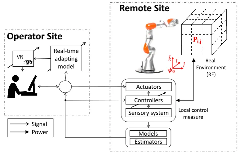
Since the main objective of this research hovers around the slave side of a typical bilateral teleoperation scheme - as in figure 1.3 - the operator contribution together with the related haptic feedback capabilities will not be addressed anymore. For instance, the supposedly arbitrary commanded motion of the operator is replaced by a generated reference path (GRP) the robot follows to approach and to interact with the real surrounding.

Thereafter, the above mentioned physical properties will be recursively estimated2from the knowledge of the reference kinematics, the measured forces and mathematical models that describe the contact phenomena.

Real-time adapting

model Ƹ𝑖 Ƹ𝑗

෠ 𝑘 𝝍𝟎

Models Estimators

Actuators

Controllers

Sensory system

Operator Site

Remote Site

Real Environment

(RE)

Local control measure

Signal Power

VR

[image:15.595.74.460.286.531.2]

𝐏

_𝐢,𝐣

Figure 1.3:The main focus of this work will be on the slave side.

Bottom line

Eventually, this work aims to:

• a fitted 3D mappingMp=[Bi,j,Bi,j,µi,j]∀Φ0Pi,jof the dynamic properties, estimated

by means of physical interaction robot/environment;

(16)

• a mapping Mv ∈ Rn ∀ 0Pi,j, which defines the point-wise (or averaged) visual

distinguishing features∀0Pi,jof the physical surrounding.

For the sake of simplicity, the geometry of the real environment is assumed to be known in advance; in particular, a flat surface has been selected.

Ultimately, all these pieces of information lead to outline an intuitivemodus operandiwhich can help to push the environment recognition matter a bit more toward the AI trend. In fact, all these data sources can be overlapped in order to find characteristic patterns inside the visual data such that those physical properties can be foreseen in alike circumstances. This approach aims to avoid likely destructive physical interactions, especially when dealing with delicate environments (e.g. biological tissues).

1.5 Related work

Within this area of study, it is right and proper to mention (Hogan,1985), in which the author coined the impedance control concept; it is considered the baseline upon which many modern frameworks in telerobotics are built upon.

In (Ueberle et al.,2009;Sheridan,1989,1993;Hokayem and Spong,2006), extensive surveys about teleoperated systems turn out to give an overview of the current state of affair about the topic.

It all comes to the measure of performance of the system, namely stability and transparency. The former concept has been the main topic in (Colgate and Brown,1994;Hannaford,1989b) - seen in its classical fashion - while Franken et al. presented a novel passivity theory in (Franken et al.,2009,2011) to deal with energy bounded systems. The concepts of bilateral teleoperation and impedance reflection (IR) method have been introduced in (Hannaford,

1989a;Hannaford and Fiorini,1988), relevant references for many of following researches into this area of study.

From that, adaptive impedance control architectures have been studied and implemented in (Velanas and Tzafestas,2010;Tzafestas et al.,2008;Abdossalami and Sirouspour,2008;Love and Book,2004;Na and Vu,2012;Misra and Okamura,2006), among others.

Besides, the estimation of the physical properties of the environment has been carried out in (Biagiotti and Melchiorri,2007;Yamamoto et al.,2008;Diolaiti et al.,2005;Haddadi and Hashtrudi-Zaad,2008,2012).

Virtual environment, in the form of augmented reality (AR) of virtual reality (VR) are by now important topics in Robotics and its research is fueld by different industries; in (Jeon and Choi,2009,2010), the authors lay down definitions and applications.

(17)

Although the current state of the art does not permit all of these EPs at the same time, such a classification helps to break down the problem and to address them singularly. Among the other variables, the vigour with which the operator holds the haptic device has important consequences to the overall performance of the system (Velanas and Tzafestas,2010). For instance, a model adaptive reference control (MRAC) to compensate for dynamics forces caused by the hand was proposed in (Na and Vu,2012).

When it comes to contact models, in (Hunt and Crossley,1975) a neat and clear treatise highlights the superiority of such a novel description over other used model. Besides, Gilardi et al. made an insightful survey in contact dynamics modelling in (Gilardi and Sharf,2002), comparing the Hunt-Crossley model with others.

How to face with friction and model it in telecontrolled systems is the core of (Bicchi et al.,

1993), whereas in (Siciliano and Khatib,2016) a later survey overarches upon its historical background and the modern approaches to deal with it.

1.6 Outline of the report

(18)

2 Background

2.1 Impedance & admittance 2.1.1 Device type

In (Hogan, 1985), the author discerns a device type classification from causality considerations: for instance, in any physical system, power instantaneously flows from one "point" to the other (e.g. robot/environment interaction) if a state variable varies. As the power is the product of two conjugate variables, namely effort and flow, any system can impose a force or a displacement (or velocity) separately, keeping the manipulator example. system along each DOF, and (Ott et al., 2010), for example. From that, Hogan distinguishes admittance and impedance type for every physical system: the former accept effort and release flow whereas the latter behaves in a dual way. Moreover, to ensure physical compatibility, in any dynamic interaction there has to be an impedance and an admittance system. And when it comes to manipulative tasks, the environment contains inertia and/or kinematic constraints, i.e. admittance type systems as seen from the manipulator point of view; hence, the manipulator behaves as an impedance. In (Ott et al.,2010), the authors outlined typical pros and cons for the two types.

2.1.2 Impedance controller

In a very trivial fashion, as already mentioned, achieving full transparency would mean having a slave robots which perfectly and timely follows the master position, that isFm =

−Fs. To this end, a possible controller design is the one presented in (Stramigioli, 1998).

It calculates the correcting torques by means of a wrenchW0,ee into the reference frame, which is proportional to the difference in between the set-point position and the end-effector location as there was a mechanical spring in between the master and the slave devices. Herein, the assumption is that both of them are impedance type. Referring to figure 2.1, it obeys to the relation:

Fs=Kv(xm−xs) (2.1)

whereFm,Fu andFs are the master, user and slave controller output forces, respectively. In

(Nijof,2018), an extension of this concept with an added damping effect is described (viz. joint damping).

(19)

CHAPTER 2. BACKGROUND 11

2.2 Bilateral teleoperation scheme

Back in 1989, Hannaford (Hannaford, 1989a) introduced a two-ports hybrid model for teleoperated systems. Human operator and environment are fully described analysing the power conjugated efforteh/e(forces) and flow fh/e (velocities) variables (Broenink,1999). By

choosing the two dependent/independent variables, one isde factoimposing the causality of the constitutive equations which describe the system. For example, when the force at position are available at the slave side, the two-port hybrid formulation becomes1:

" eh fh # = "

h11 h12

h21 h22

# "

fe ee

#

(2.2)

However, when interaction occurs, the position of the slaveqe=d f_{d t}e can be correlated to the

forceFevia the multivariable impedance functionZe (Lawrence,1992), which, in principle,

can have an arbitrary form alikeFe=Ze(qe). Then, for the sake of simplicity, the linear case

is considered such that:

Fe=Zeqe (2.3)

Therefore, thehi jvalues into the system 2.2 can be interpreted as:

T

ee

fe eh

fh

Z

e

Z

_h

Human hand model

OPERATOR CONTROLLED SYSTEM TELEOPERATOR ENVIRONMENT

Figure 2.2:Two-ports model of a teleoperated system.

Hh ybr i d=

"

h11 h12

h21 h22

#

=

"

Ze KF Kv _Z1

h

#

(2.4)

whereKFandKvare force and scaling factors respectively. Taking advantage of this notation,

one can rephrase the ideal transparency concept in terms of:

eh=ee fh=fe

(2.5)

It happensiff the impedance transmitted to the operatorZh is equal to the one showed by

the environment, that is:

Zh=Ze (2.6)

It comes from here this concept the impedance reflection (IR) definition. Solving the system 2.2 forehandfh, and using equation 2.6, then:

eh=(h11−h12Ze)(h21−h22Ze)−1

| {z }

Zh

fh

(2.7)

1_{Everything is described within the frequency domain (Laplace transform) and the complex operator "s" is}

(20)

T

ideal teleoperator

Z

e

ee

fe

eh

fh

Z

e

Z

_h

Figure 2.3:Transmitted impedance.

This relations claims that perfect transparency occurs iff h11 = h22 = 0 ∧ h21 = −h12, confirming that thehmatrix for an ideal teleoperator looks like:

hi d eal=

"

0 1

−1 0

#

(2.8)

The same reasoning can be applied at the slave side if the "human hand impedance"Zhwere

considered. Eventually, in (Hannaford,1989a), the "bilateral impedance control architecture" has been proposed: both sides of the teleoperation scheme are equipped with a local control law which enforces estimated impedance and force of the other side. It is worthy to mention that such a two-port model, is a linear system, hence valid only around equilibrium points; for example, non-linear delaying terms e−sτ should be addressed differently (Hannaford,

1989b).

Figure 2.4:Conceptual scheme of the IR in teleoperation.

2.3 Haptic rendering architectures

Haptic rendering algorithms evaluate the interaction forces between the haptic interface representation inside the virtual environment and the virtual objects inside it (Salisbury et al.,

2004). Figure 2.5 exemplifies this algorithm:Sstands for the contact,Xis the position,Fdthe

(21)

[image:21.595.234.322.419.617.2]

CHAPTER 2. BACKGROUND 13

Figure 2.5:Haptic rendering scheme.

2.4 Experimental setup

2.4.1 Hardware

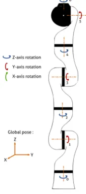
KUKA LWR

Within this investigation, a 7 DOF serial robotic arm KUKA LWR4+ has been employed, as schematically reported in figure 2.6. An internal robot controller (KRC) is connected via UDP to an external computer, and it provides features to compensate for friction and gravity. For instance, through the latter, a set-point could be commanded to the internal impedance (or position) controller, or joint torques as resulting from an external controller.

Due to time constraints, the same implementation as in (Nijof,2018) has been considered:

Figure 2.6:KUKA LWR joints.

for instance, the widely used C++ library FRI2allowed to command position setpoints, while running an external impedance controller with aKc=5200.

(22)

End effector

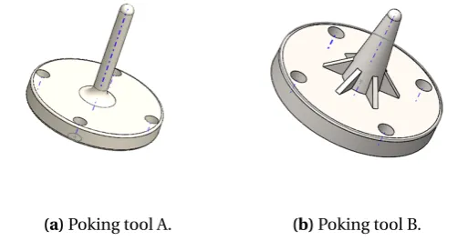
A blunted end-effector has been purposely designed in order to let the robot interact with the surrounding environment, in such a way to allow smooth poking and surface following (i.e. sliding) motions. Figure 2.7 show the two used tools, whereas the second (rendering 2.7b turn out to be a better design for the purpose: that was because of its stocky shape. In appendix A.2 its he mechanical design is attached.

In between the robotic arm and these tool, a force-torque sensor (ATI MINI40-E3) has

[image:22.595.188.445.222.360.2]

(a)Poking tool A. (b)Poking tool B.

Figure 2.7:Poking tools.

been mounted in order to measure the extent of the dynamic interaction with the real environment.

2.4.2 Software interface

In a modular fashion, commanded set-points, controlled output torques and measured forces/torques are monitored within a ROS4 environment. For instance, the commanded set point, the FRI interface, the impedance controller and the force sensor correspond to differentnodes. In turn, they exchange messagesthroughtopics using the publishing and subscribingstructure, so as to synchronise themessagesand embed all the modules within a single environment.

3_Source:_website.

(23)

15

3 Problem analysis

Looking at a typical teleoperation scheme, from the control standpoint, it is well known that a solely force or position control do not suffice for constrained tasks (Erickson et al.,2003); that is the main reason why the impedance control strategy (in its general accepted meaning) proposed by Hogan (Hogan,1985) is so widely applied. In fact, it aims to adjust both position and force at the same time, when a dynamic relation in between them is superimposed within a single control law (section 2.1). In the most general case it is expressed in a matrix form, so as to address the contribution of each Cartesian variable with respect each other; however, under the simplifying assumption of uncoupled relations, the study can be circumscribed to a single relation.

It has been shown in (Love and Book, 1995) and (Seraji et al.,1996), among others, that when the mechanical properties of the RE are known, the teleoperated system performs better. Knowledge of the environment can be used to optimise control, and having reliable estimates for stiffness and damping coefficients of the physical surrounding, would allow the implementation of more advanced control schemes (Love and Book,1995). It turn out to better track the reference force and to improve the stability margins of the impedance controllers: i.e. transparency and stability performance would enhance.

With the aim of implementing the IR approach (section 2.2) within further investigations, the goal here is to recursively estimate the impedance of the environment -Ze, namely stiffness

and damping- so as to be used, for example, into the local master controller or to build up a more realistic VR world.

The first step toward the implementation of an online impedance estimation of objects interacting with a robotic device is the choice of a suitable contact models (Erickson et al.,

2003).

3.1 Contact models

This section will briefly recall some physical models to describe the interaction in between two bodies, where the first is rigid (slave’s end-effector), the second visco-elastic (the real environment). Generally speaking, a model is the first guess scientists use to describe and predict the behaviour of the real world; then, within an iterative and correcting cycle, an experimental validation phase would confirm - or not - its suitability.

3.1.1 Assumptions

In some previous researches (Love and Book, 1995;Hashtrudi-Zaad and Salcudean,1996) the inertia of the poked body has been estimated too. However, a rather typical assumption in telemanipulation is to consider the teleoperated system to behave through a sequence of equilibrium states. It follows that the sum of all the forces acting upon the body is null. This quasi-staticassumption describes a "slow" evolution of the system and it allows to neglect the inertial effects.

(24)

Figure 3.1:Point-wise contact.

point-wise (ideal) contact. The resulting forceFeapplied by this point can be decomposed in

a tangential, radial and normal components w.r.t. the areaA, such thatkAk→0. That is:

Fe=Fnn+Ftτ+Frr (3.1)

Therefore, assuming persistent contact and isotropic material properties within the planeπ spanned by the versors ˆr and ˆτ, would simplify the problem to consider solely the normal componentFn, acting upon the centroid as sketched in figure 3.1. Eventually,

Fe=Fn (3.2)

From now on, the direction of the environmental forceFe will always be the same as ˆn, and

the vector notation will be replaced by the scalar one.

How this Fe is modelled will be the topic of the following paragraphs: in fact, stiffness,

damping and friction coefficients will be illustrated within typical idealised structures.

3.1.2 Linear models

Hooke

The simplest way to modelFn within a virtual environment scenario, for example, is the

linear position dependent case. Firstly the point-wise collision is detected, then the haptic interaction point (HIP) -using the same nomenclature as in (Ho et al.,1999)- penetrates the virtual object surface; finally, a commonly used reflected forceFe obeys to theHooke’s law:

Fe(t)=FHooke(x)=







0 x(t)≤0

kx x(t)>0 (3.3)

(25)

[image:25.595.184.381.105.228.2]

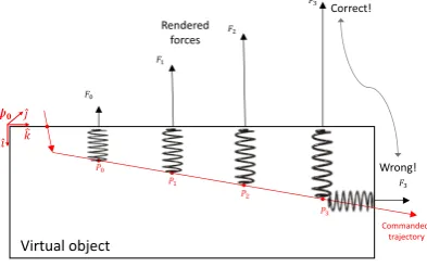
CHAPTER 3. PROBLEM ANALYSIS 17 Virtual object Commanded trajectory 𝑃0 𝑃1 𝑃2 𝑃3 𝐹0 𝐹1 𝐹2 𝐹3 𝐹3 Correct! Wrong! Ƹ𝑖 Ƹ𝑗 ෠ 𝑘 𝝍𝟎 Rendered forces

Figure 3.2:Rendered forces.

contemplated within this representation. Although its apparent simplicity, as noticeable from figure 3.2, this model still needs special attentions.

After all, regardless of the adopted model, the resulting rendered forcesF, evaluated within the Cartesian space, have to be translated in torques τ applied by the actuators of an hypothetical haptic device. To accomplish that, the transformation

τ(t)=JTFe(t) (3.4)

is used, whereJis the Jacobian matrix of the specific haptic device.

Kelvin-Voight

The pure elastic model can be modified to incorporate other effects, for instance the contribution of an added Newtonian damper. A simple implementation, more commonly known as Kelvin-Voight model, sees a parallel connection in between a spring and a damper; besides, the so called Maxwell and Zener configurations are two other linear ways to ascribe for other physical effects (Biagiotti and Melchiorri,2007).

Fe(t)=FK V(x, ˙x)=







0 x(t)≤0

kx(t)+dx˙(t) x(t)>0 (3.5)

However, in (Gilardi and Sharf, 2002), the authors summarise the weaknesses the Kelvin-Voight model suffers from:

• as soon as the impact takes place,Fe is discontinuous because of the damping term,

and the same happens when the probe looses the contact with the environment. Intuitively, for x=0, both the elastic and viscous components should be null while increasing over time;

• during the rebound phase, as the penetrationx_→0, a negative force holding the bodies together is predicted by this model;

(26)

No matter how, for many practical applications, regardless the above mentioned physical inconsistencies, this model is still very simple (great asset) and predicts reasonably the energy dissipation, unconcerned about plastic deformation matters.

The coefficient of restitutione, defined as

e=vo vi

(3.6)

gives an idea about the energy dissipation during the (1 dof ) impact in between two rigid bodies. In equation 3.6, vo and vi are the relative velocities after and before the contact,

respectively. It has been shown (Hunt and Crossley,1975) that for lowvi, and inside the

elastic range of the material, thenecan be approximated by:

e=1−αvi (3.7)

whereαis a (low-value) constant, depending on the material and the geometry of the surface in contact.

3.1.3 Non linear models Hertz

The shortcomings of the Hooke model, can be overcome considering a non-linear elastic force as:

Fe(t)=FHer t z(x,n)=







0 x(t)≤0

k x(t)n x(t)>0 (3.8)

where the constant exponentnvaries with the material and the shape of the colliding objects. Additional assumptions upon which this model has been derived are (Gilardi and Sharf,

2002):

• the deformation is concentrated in the proximity ofA;

• the elastic wave motion is disregarded;

• the inertia of each of the body is concentrated into their centers of mass.

For completeness, equation 3.8 could be upgraded with additional terms to take into account other phenomena: e.g. hysteresis and plastic deformation.

Hunt-Crossley

Using the previously presented models as building blocks, in order to take into account also the energy dissipation, while keeping coherency with the coefficient of restitution, in (Hunt and Crossley,1975) the Hunt-Crossley model has been proposed as follows.

Fe(t)=FHC(x, ˙x,n)=



0 x(t)≤0

(27)

CHAPTER 3. PROBLEM ANALYSIS 19

The "new" parameters are commonly chosen asp=nandq=1.

The main advantage of this model is to have a damping component of the normal force which depends on the extend of the penetrationx,de factoeliminating those discontinuities at the beginning and at the end of the contact, which are instead present in 3.5.

Using this model, the parameterαin equation 3.7 can be approximated by:

α=2d

3k (3.10)

therefore solely depending on material properties. In (Diolaiti et al., 2005; Haddadi and Hashtrudi-Zaad, 2008, 2012) it has been proved that this model clearly outperforms the Kelvin-Voight one for softer real environment types (e.g. biological tissues).

From these observations, within this research, the Hunt-Crossley model would be the preferred descriptor of the interaction in between the slave robot and the surrounding physical environment.

3.2 Friction models

Friction is commonly interpreted as the resisting force which arises in between two contacting bodies with non-null relative velocity v. It is a complex and highly non-linear phenomenon for which empiric formulations are often used from case to case. While robotics still lacks of advanced skin-like tactile sensor availability1, frictional forces are essential to carry out human-like dexterous manipulations; for example, to control the level of slippage. Additionally, moving frictional information within a virtual world model, would extend its overall description and lead to a more realistic experience to the user on the ground that more senses would be stimulated. While friction is often an undesired phenomenon (e.g. in high-precision mechanisms), other times is pursued (i.e. 3D scanners, tyres manufacturing, grasping tasks); however, in both cases, a thorough understanding of this phenomenon would lead to optimised solutions.

In many dexterous manipulations, slippage is seen as an undesirable loss of control, therefore the main concern is about the static friction limits (Bicchi et al.,1993). Therefore, a static friction model, solely dependent onv, will be herein used and validated -or not- within the production phase.

The most common model is built upon the Coulomb friction and a linear viscous damping components, while neglecting adhesion and addressing only (1 dof ) compressive forces, such that:

Ff r i c=FC oul omb+FK i net i c=

=µstFnsign(v)+µki nv

(3.11)

This model can be used to roughly model friction forces for steady-state velocities (Van Geffen,2009), not close to zero. Specifically,Fnstands for the normal compressive force

and the coefficientsµst,µki n depends on the material properties as well as the geometry of

the object in contact. Furthermore, to describe the empirical occurrence of lower friction forces as velocity increases within a bounded region (figure 3.3b), the StribeckeffectFSt r

could be added to equation 3.11. For the sake of thoroughness, more advanced descriptions,

(28)

such as the "seven parameters" model,DahlandLuGreones could be considered to take into account other physical details. Hence, looking at figure 3.3a, "far enough" fromv=0, one could expect a constant friction force for constant relative velocityv. Due to its simplicity,

Ff r iction [ N ]

V elocity m

s

(a) Static, Coulomb and kinetic friction. Ff r iction [ N ]

V elocity m

s

FSrtibeck

(b)Stribeck friction model.

Figure 3.3:Simplistic frictional behaviours.

equation 3.11 was chosen as default for further experiments.

3.3 Estimation

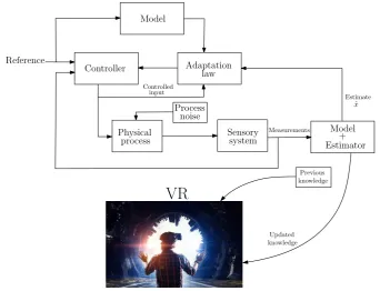
Referring to figure 3.4, and as mentioned in section 1.3, having available trustworthy information about the remote environment would lead to the double benefits of :

1. improving transparency and stability (Diolaiti et al.,2005;Misra and Okamura,2006;

Franken et al., 2011; Hannaford, 1989b; Colgate and Brown, 1994; Hannaford and Fiorini,1988;Yamamoto et al.,2008;Biagiotti and Melchiorri,2007);

2. extending the virtual reality paradigm as in figure 3.4 with meaningful physical properties of the real environment. It would yield to a more realistic VE itself and to more realiable haptic reflected forces (haptic rendering); an high-level framework for automatic property identification is presented in (Dupont et al.,1999).

(29)

Adaptation law Controller

Controlled input

Measurements

VR

Reference

Model

Estimator+ Estimate

^ x

Updated knowledge Model

Physical

process Sensorysystem

Process noise

[image:29.595.108.451.99.361.2]

Previous knowledge

Figure 3.4:Adaptive control scheme with VR.

3.3.1 Least square

Any model that is linear in the parametersθi, can be written as a linear regression:

yi=φ1(xi)θ1+...+φn(xi)θn+ei=

=φTθ+e (3.12)

where:

• y=£y1, ...,yN¤T is the measured output vector, function of the observable statesxk;

• e=£e1, ...,eN

¤T

is the error vector. It takes into account the uncertainties inθ;

• θ=£

θ1, ...,θN¤Tis the parameter vector;

• φ=£

φ1, ...,φN¤T is the regression vector;

Therefore, this estimation problem aims to estimate -offline- the vector ˆθwhen some cost function ofV(e) is minimised (for a more detailed analysis, the interested reader should take a look at (Ljung,1998)).

IfφTφexists and it is non singular, the parameter vector is the unique solution:

ˆ

(30)

3.3.2 Recursive least square

When the interest moves to estimate in real timeθ, in other words updatingθi−1 when the values©

yi ,xiªare measured, then a recursive formulation is needed.

Ljung et al., in (Ljung,1998), illustrated how to use theinversion lemmato accomplish so, elegantly demonstrating that the online estimated parameters ˆθican be evaluated by:

ˆ

θi=θˆi−1+Ki

³

yi−φTi θˆi−1

´ (3.14) where     

Ki=Pi−1φi

³

1+φTiPi−1φi

´−1

Pi=

³

In−KiφT_i

´

Pi−1

(3.15)

From equation 3.14, it is worth nothing that the new estimate ˆθi is equal to the previously

evaluated ( ˆθi−1) corrected by the term

³

yi−φT_iθˆi−1

´

, i.e. the single-step prediction at the time (i−1).

Moreover, the initialisation problem for P0 (equation 3.15) can be dealt by admitting a small initial error ² ¿ 1 such that P0 = 1_²In. Besides, a variation of the RLS method,

namely exponentially weighted recursive least square (EWRLS) can help to deal with varying parameters (Love and Book, 2004;Erickson et al.,2003). It can be achieved by tuningwi

inside the expression of the cost functionV(ei)=P_iN₌₁wie2_i, therefore the covariance matrix Pi, so as to value more the latest measurements w.r.t. the older ones (Biagiotti and Melchiorri, 2007). This new recursive formulation is therefore reported beneath:

               ˆ

θi=θˆi−1+Ki

³

yi−φTiθˆi−1

´

Ki=Pi−1φi

³

β+φTi Pi−1φi

´−1

Pi=

1 β

³

In−KiφT_i

´

Pi−1

(3.16)

where the forgetting factorβ∈[0.95−1] takes care of these variations, the lower its value, the more the parameters varies.

3.3.3 Recursive Hunt-Crossley estimation

Using the Hunt-Crossley model (section 3.1.3), and assuming available force measurements as well as position and velocity and the end-effector, estimating the physical properties of the environment means findig the valuesnkˆ, ˆd, ˆno2.

Double stage identification

In (Biagiotti and Melchiorri,2007;Diolaiti et al.,2005) the author proposed a two stages RLS estimation by defining two estimatorsΓ1andΓ2as in figure 3.5. The vectors to applied the

(31)

Γ1(x;x; F;_ n^)

[image:31.595.198.362.100.196.2]

Γ2(x;x; F;_ ^k;d^) _n_^ (^k;d^) (x;x; F_ )

Figure 3.5:Online two stages estimation for the Hunt-Crossley model as in (Diolaiti et al.,2005).

recursive formulation 3.16 were defined as:

Γ1:

           ˆ θ1=

h

ˆ k, ˆdiT

φ1=£xn,xnx˙n¤T

y1=£FHC¤

(3.17)

Γ2:

             ˆ θ2=£nˆ¤ φ2=£l og(x)¤

y2=

"

l og

µ _F

HC k+dx˙

¶# (3.18)

This method has experimentally proved to be sound: convergence to the true values is obtained under strict assumptions about the nature of the error, material properties and initial values for the estimates ˆθiwhile using an had-hoc forgetting factorβ.

Single stage identification

In (Haddadi and Hashtrudi-Zaad,2008), Haddadi et al. presented a novel way to estimate recursively the parameters of the Hunt-Crossley model using a one-step procedure. A thorough analysis about the weaknesses of the previously two-stages method revealed that although it leads to convergence, it is very sensitive to parameter initial conditions and dynamic properties variations.

Recalling equation 3.9, forx>0 it has been shown that:

FHC(t)=k x(t)n+dx˙(t)x(t)n+² (3.19)

(32)

From equation 3.19, the readers will agree on the equivalence3:

l n¡

FHC¢=l n



k xn Ã

1+dx˙ k +

²

k xn

!

=

=l n(k)+n l n(x)+l n

Ã

1+dx˙ k +

²

k xn

!

| {z }

1+α

(3.20)

With the aim to linearize equation 3.19, the Maclaurin expansionl n(1+α)→α+O(α2) if α→0, could be a tool. Hence, it has to hold that:

|α| =

¯ ¯ ¯ ¯ ¯

dx˙ k +

²

k xn

¯ ¯ ¯ ¯ ¯ ≤ ¯ ¯ ¯ ¯ ¯

dx˙ k ¯ ¯ ¯ ¯ ¯ + ¯ ¯ ¯ ¯ ²

k xn

¯ ¯ ¯

¯→0 (3.21)

The last inequality implies that both the terms¯¯ ¯

dx˙

k ¯ ¯ ¯and ¯ ¯ ¯ ²

k xn

¯ ¯

¯should be "small enough". As

a rule of thumb, the former can be solved bounding the velocity to the condition:

kx˙k∞<0.1

k

d (3.22)

On the other hand, the latter can be overcome by fixing a minimum penetration so as to satisfy for example:

° °xn

° °

∞>B

²

k (3.23)

where the constantB has to be≥10, in order to neglect the process noise term in equation 3.19.

As a matter of fact, both these conditions depends on the properties of the environment and on the power of noise. Although both reasonably achievable, they have to be checked within the experimental phase.

Upon the above constraints, equation 3.19 becomes:

l n¡

FHC

¢

=l n(k)+n l n(x)+dx˙

k (3.24)

hence a linear system, and the EWRLS estimation (equations 3.16) can be applied using the vectors:

ˆ θ=

"

l n( ˆk), dˆ ˆ k, ˆn

#T

φ=£

1, ˙x,l n(x)¤T

y=£l og(FHC)

¤

(3.25)

This method has been experimentally validated in (Haddadi and Hashtrudi-Zaad,2012) and its superiority w.r.t. the two stages procedure proved.

(33)

3.3.4 Friction coefficients estimation

From the linear model 3.11, and using the same nomenclature as in section 3.3.1, the following vectors are defined :

ˆ

θ=£µˆst, ˆµki n

¤T

φ=£Fx, ˙y¤T y=hFy

i

(3.26)

The same can be used to run a RLS estimation, i.e. equation 3.16.

Persistent excitation

To achieve the convergence of ˆθ to the true value(s), an important role is played by the richness of the input signal to the process. This concept, more commonly referred to as persistence of excitation (PE), stands to express the qualitative notion that the input signal to the plant should be such that all the modes of the plant are excited (Narendra and Annaswamy,2012).

Specifically to the above mentioned case, three parameters have to be estimated ³kˆ, ˆd, ˆn´, hence as a rule of thumb (Slotine and Li, 1989), a reference signal containing two sine functions should be enough. However, the non linearity effect due to the logarithmic function in 3.24, should lead to convergence already with a single periodic reference signal (Haddadi and Hashtrudi-Zaad,2012). These claim has been confirmed in (Yamamoto et al.,

2008), where the authors compared three different level of excitation so as to determine the minimal requirement for convergence: one sine function turn out to be enough.

(34)

4 Design and implementation

4.1 Simulations

From a feasibility aspect, simulations are carried out to confirm the allegations from the previous chapters. Firstly, simulations have been carried out using constant parameters K(t),B(t) andn, where the estimated values immediately converged to the real ones. Because of that, other simulations have been made more realistic considering varying physical properties (linearly w.r.t. the simulation time), such that:

K(t)=100+10t B(t)=10+1t

n=1.2

Besides, in order to make the input signal a persistant excitation, a multi-sine reference established the interaction along the perpendicular direction in between the end-effector of the robot and the real environment, as it follows:

z(t)=0.012si n(2π2t)+0.003si n(2π5t)+0.021

Figure 4.1 reports the imposed kinematics of the end-effector, meant to represent the punctual trajectory of it as it was translating along the z-axis. The last terms guarantees that z(t)>0∀t, i.e. a superimposed contact, while two modes of the environment are excited. Additionally, to make the simulation more realistic, a white noise withSN R=40 enriches the frequency content of the reference signalz(t). For the sake of curiosity, the FFT ofz(t) has been attached into the appendix figure A.1.

Time [s]

Figure 4.1:Simulations: reference kinematics.

4.2 Experimental phase

(35)

CHAPTER 4. DESIGN AND IMPLEMENTATION 27

instability, has been set.

As a matter of fact, although this precautionary measure, the robot has behaved in a rather soft manner, potentially far away from an position controlled setup: the consequences of that will be clarified within the following sections.

4.2.1 Methodology

From the previous chapter, referring to figure 4.2, this research aims to achieve the mapping:

Mp:={ ˆK, ˆB, ˆn, ˆµst, ˆµki n}∀Φ0Pi,j (4.1)

With this goal in mind, the end-effector of the slave robot will "scan" the environment in

Slave Robot

F_sl v_sl =const

End-e_ffector

6 dof Force sensor

+

F_R

Φ

0

z

x

y

P_x;y ^

k

^i

^

j

Figure 4.2:Procedure and physical properties mapping.

order to evaluate its physical properties, namely stiffnessK and damping coefficientB, the adimensionaln(only for HC model) and the friction parametersµstandµki n, all function of

the only planar coordinates¡x,y¢₁

.

For the purpose of estimatingK andB, perpendicularly w.r.t. A(figure 3.1), the end-effector of the robotic manipulator will interact with the real environment by means of an orthogonal poking motion: i.e. a punctual excitation. From that, the triad ˆK, ˆBand ˆn or the pair ˆK, ˆB will be evaluate using the HC and/or KV contact model, respectively.

Such an approach will be iteratively repeated a sufficient number of times N, so as to end up with N triads ˆK, ˆBand ˆnor the pairs ˆK, ˆB.

On the other hand, another trajectory will be commanded to the Kuka arm to estimate the friction coefficientsµst andµki n in between the tip of the end-effector and the surface

-planar, for simplicity- of the environment, sliding from one point to another (figure 4.6). For instance, once the static value of the friction is overcome, the end effector will start sliding upon the surface, maintaining a constant penetrationz(t)and velocityvsl(t). At this point,

(36)

the two dynamics of poking and sliding, although coupled, can be in part associated to the normalFn(t)and planarFsl(t)components of the measuredFR(t)respectively. Under this

conditions, and within the kinetic range of friction (section 3.2), bothFnandFslare expected

to be overall constant; if it is not the case, at least one of the previous estimates changes value, i.e. the material properties are discontinuous. Hence, by uniquely monitoring the evolution ofFnandFsl during such a gliding, one can get a grasp about when/where the RE changes

its physical properties.

4.3 Experiment design

4.3.1 Elastic environment

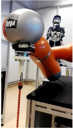
[image:36.595.251.379.292.517.2]

The easiest tested scenario has been a, allegedly, chiefly elastic environment: for instance, a tense elastic band has been attached at the tip of the end-effector, in line with the poking direction and perpendicularly w.r.t. the ground (figure 4.3). Insightful outcomes

Figure 4.3:KUKA arm interacting with an elastic environment.

about the setup limits, models complexity, and estimation procedure turn out by means of experimenting onto thisquasi-elastic environment. As a matter of fact, from a trivial static experiment, and applying Hooke’s law, the expected stiffness of the band was around 88 _mN. Subsequently, in order to estimates the longitudinal properties of the RE, the elastic has been pretensioned to such an extent that for the minimum elongation (0.045m), a residual tensile stress was still present (no flaccid behaviour).

In the end-effector coordinates, the commanded displacements obeyed to the relation:

x(t)=0 y(t)=0

z(t)=0.025si n(2π1.7t)+0.010si n(2π4t)+0.08

(37)

However, even though the short stroke and the soft environment, poor tracking performance of the employed setup were evident. For the sake of thoroughness, figure 4.4 demonstrates this observation, while it is worth mentioning that it does not represent a real problem since the goal of this research differs from fine manipulative tasks.

While the elastic force exerted by the environment would push the end-effector’s tip toward

Time [s]

Position [m]

Figure 4.4:Elastic environment: position set-point tracking.

the negative direction, the robot does not apply enough torques to reach the higherz(t). From that, it is obvious the existing trade-off among the level of pretension (Fe) and the

tracking performance. While the latter does not affect the models fitting (positions and forces are still available), it turn out to be trickier to reach a persistent excitation, as needed to perform an online estimation (section 3.3.4).

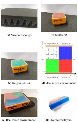
4.3.2 Viscoelastic environment I: anechoic sponge

A similar set of experiments as for the quasi elastic environment have been carried out using a anechoic sponge (figure 4.5a) to mimic another kind of plausible RE scenario. Furthermore, the experimental procedure has been standardised for both the poking and sliding movements - not integrated but independently executed - as it follows:

- Phase I - the tip of the end effector slowly moves closer to the material surface and penetrates the material for the desired depth (constant velocity phase, lasting≈5s); - Phase II -a standing phase (null velocity, lasting≈1s) has been placed so as to get rid

during the data processing phase of possible bias in the force sensor measurements, prior the experiments start;

- Phase III -poking or sliding motion, depending on the wanted properties, takes place following specific commanded trajectories;

- Phase IV - phase I is reversed and the residual penetration is removed (z(t)=0); - Phase V - the original position is reached (x0/y0, only for sliding).

Poking

(38)

completeness, the interaction took place at the geometric centre of the surface (4x4cm) of the rubber.

x(t)=0 y(t)=0

z(t)=0.003si n(2π0.9t)+0.001si n(2π5t)+0.012

(4.3)

Sliding

In order to observe a behaviour similar to figure 3.3a, the friction coefficients determination is based on the assumptions that the penetration inside the material is constant. For instance, w.r.t. the material surface, the following motion profile - during phase III - is commanded:

x(t)=0 y(t)=0.003t z(t)= −0.0025

(4.4)

Moreover, during this phase, a constant orientation is imposed to the last joint of the robot, viz. the end effector is always perpendicular w.r.t. the material surface.

4.3.3 Viscoelastic environment II: smooth-onEcoflex 50

Thus, in order to have a larger population of tested materials (mimicking different RE scenarios), the rubber -silicon type-Ecoflex 502, produced by Smooth-On, has been tested as in the previous case. Because of its low viscosity, softness and stretchy properties, it is often used to make prosthetic appliances and cushioning for orthotics. For purposes which will be clearer later, nonetheless, the sample has been coloured with red glitter (figure 4.5b). It is worth pointing out that due to the higher stiffness of this RE, only smaller penetration was possible (<1 cm), de facto making harder reaching a PE to recursively estimate the coefficients of the HC model. The considered reference signal was:

x(t)=0 y(t)=0

z(t)=0.0015si n(2π0.9t)+0.0005si n(2π5t)+0.003

(4.5)

4.3.4 Viscoelastic environment III: smooth-onDragon skin 10

Eventually, another silicone compound used for a variety of applications, ranging from creating skin effects to making production molds, has been employed as a RE sample: the Dragon skin 103produced by Smooth-On. From specs, this silicone is slightly stiffer than the previous one; nonetheless, to better distinguish it from the other rubber type, it has been coloured with blue glitter (figure 4.5c).

2_{Shore hardness: 00-50}

(39)

(a)Anechoic sponge. (b)Ecoflex 50.

(c)Dragon skin 10.

y

[

cm

]

10

1

x[cm] 10 1

Dragon skin 10 Ecoflex 50 Dragon skin 30 Ecoflex 30

(d)Ideal mixed environment.

[image:39.595.145.414.169.586.2]

(e)Real mixed environment. (f )Overflowed layers.

(40)

4.3.5 Mixed environment

Using the previous cases as test bench, and the corresponding outcome as a reference, a mixed RE has been prepared by placing four different types of rubbers within a square mold (figures 4.5d). Approximately each quarter of it has been filled with a liquid compound, differently coloured, as it follows:

• Ecoflex 304- blue; • Dragon skin 305- white; • Ecoflex 50- red glitter; • Dragon skin 10- green glitter.

During the preparation, due to the different viscosity of the liquids, the compounds slightly mixed up, making the RE even more interesting: in particular, the blueEcoflex 30(out of all, the softest silicone from specifications) overflowed upon theDragon skin 30(the stiffest one, on paper). Figures 4.5e and 4.5f show this effect into the final solid compound.

Poking

A grid with 10x10 little squares, meshed using 1x1cmlinks, has been virtually drawn to carry out 100 point-wise poking procedures, to partially estimate the mappingMp of this mixed

RE. From those experiments, the effect of the "rigid" border of the mold, and an ambiguous behaviour due to the mixed fluids are expected to arise during the data processing phase.

Sliding

Figure 4.6 shows the paths which have been followed by the probe to determine if any force leap occurs when sliding upon the RE’s surface. In particular, the bold and labelled arrows are used as the representative trajectory to shows the most relevant transitional behaviours from one type of silicone to the other. During this gliding phase, the set-point trajectory of the probe obeyed to the relations:

x(t)=0 x(t)= −0.002t y(t)=0.002t or y(t)=0 z(t)= −0.0025 z(t)= −0.0025

(4.6)

depending on the direction of the sliding, as sketched in figure 4.6. Moreover, during this phase, a constant orientation is imposed to the last joint of the robot, viz. the end effector is always perpendicular w.r.t. the material surface.

4_{Shore hardness: 00-30}

(41)

y

[

cm

]

10

1

x[cm]

10 1

Dragon skin 10 Eco_flex 50

Dragon skin 30 Eco_flex 30

3

4

1

[image:41.595.177.383.100.317.2]

2

Figure 4.6:Mixed environment: grid and sliding paths.

4.4 Visual identification

Within this section, an hint to the recognition of the physical properties of the real environment via the only visual data is made. So far, the triad of valuesMp:={ ˆK, ˆB, ˆµeq} is

aimed by enforcing the end effector of the robot to penetrate - up to a controlled extent - the surface of the real environment. Such a situation, however, is not always feasible and it can be a risk when dealing with fragile or exploding environments, for example. Furthermore, as described in the previous sections, evaluating the mapping Mp is a rather long-lasting

procedure.

4.4.1 Concept

(42)

Figure 4.7:Mixed environment and its RGB components.

Since the mapping of the dynamic properties would be known, the aim is to train the system so as to immediately extract a first guess about the nature of the these physical characteristics from the solely RGB image.

From this preamble, the following implication is investigated:

{ ˆK, ˆB, ˆµeq}←→? {R,G,B, }

(43)

35

5 Results

This chapter outlines the results of this research, as they can be inferred from the outcome of the experiments as described in the previous chapter.

5.1 Simulations

Accordingly to figure 5.1, the force components of the HC model keep a positive sign, while the viscous contribution is greatly minimised w.r.t. the the same term into the KV representation. Moreover, looking at the same plots, it stands clearly how much smaller was the damping component of the HC model (negligible in this case) w.r.t. the KV description.

On the other hand, as it was predictable from the observations of section 3.1.2, negativeFB Kelvin-Voight force components

Time [s]

Hunt-Crossley force components

Figure 5.1:Simulations: forces components of the KV and HC models.

arises in the KV model, and this physical inconsistency is even more evident looking at the energy hysteresis diagram in figure 5.2.

It has been straightforward estimating ˆK and ˆBfor the KV model, using the RLS procedure:

x [m]

Force [N]

Kelvin-Voight

x [m]

Force [N]

Hunt-Crossley

Figure 5.2:Simulations: energy hysteresis diagrams.

(44)

immediate (<0.1s) convergence of the parameter vector ˆθ to the simulated values. More interesting is the recursive estimation for the linearized HC model: figure 5.3 displays the outcome.

In this case, usingβ=0.98 or an exponentially weightedβ=1−0.01e−5(t−2)(section 3.3.3),

Stiffness [N/m]

Estimated Dynamic properties

Damping [Ns/m]

Time [s]

Force [N]

Estimated force

Force [N]

Absolute error

Time [s]

Relative error

Figure 5.3:Simulations: EWRLS applied to the HC model.

does not show palpable differences (figure 5.3 illustrates the latter case). Here, the estimates converge to the simulated values after 0.3swith some bland LF oscillation (variation≤1.5%).

Assumtion check

Time [s]

Figure 5.4:Simulations: assumption validity check for the linearized HC model.

(45)

CHAPTER 5. RESULTS 37

5.2 Experiments

5.2.1 Elastic environment

The plots in figure 5.5 show the measured positions and forces when the robot interacts with an (chiefly) elastic RE. As an evidence of thequasielasticity of the environment, the third plot

Displacement [m]

Force [N]

x axis

Displ. [m] Force [N]

y axis

Time [s]

Displ. [m] Force [N]

z axis -poking

direction-Figure 5.5:Elastic environment: measured forces and positions.

suggests thequasilinear relation position/force. However, from the same figure, an evident coupling among the axis arises: along thex and y directions, in fact, displacements (and consequently forces) occur, contrary to the set-points 4.2.

As for the simulated case, applying a RLS to the KV model withβ=0.98, led straightforwardly

Recursive estimation: KV model

Time [s]

Figure 5.6:Elastic environment: online estimation KV model.

(46)

Recursive estimation: HC model

Time [s]

Figure 5.7:Elastic environment: online estimation HC model.

3.3.3), choosingβ=1−0.01e−3(t−2)_{to balance the convergence with the time to reach it. For} such a soft environment, however, a PE has been possible by increasing the amplitude of the components ofz(t) in 4.2, an unfeasible instance if the RE were stiffer though.

Furthermore, for the sake of consistency, the linearization validity has been checked and reported in the appendix figure A.3. Eventually, the output estimates from both the models

Force [N]

Output estimates: KV

Time [s]

Force [N]

Output estimates: HC

Residual: KV

Time [s]

Residual: HC

Figure 5.8:Elastic environment: estimates’ residual.

Toward spatial impedance estimation for robotic systems