Applying machine learning to the prediction of defaults in loans

(1)

prediction of defaults in loans

June 8, 2018

Author:

Michiel Cornelissen BSc. s1229532

Supervisors:

University of Twente drs. ir. Toon de Bakker dr. Mannes Poel

Accenture

Paul Weiss MSc.

University of Twente Drienerlolaan 5 7522 NB Enschede

Accenture

(2)

(3)

Management summary

The goal of this thesis is to compare the predictive performance of several machine learning algorithms in their capability to predict defaults in loans. This is done to come up with valuable information about which algorithms are most suitable for this task. Such information is required before machine learning can be implemented in practice to predict defaults. To determine the performance, several algorithms that can be used to classify samples have been implemented. Those are used to predict the defaults and the performance of each of the algorithms is measured.

The loans used in this thesis come from two data sets of which it is known which loans went into default. The choice has been made to use two data sets in order to be able to determine if the same results are found for both sets. The first data set, from the UCI Machine Learning Repository (Yeh and Lien, 2009), consists of 30,000 Taiwanese credit lines. The second data set, after preparation, is comprised of 85,964 peer to peer loans that have been originated using the Prosper platform (Prosper, 2017).

The main question of this thesis is:

What is the predictive performance of machine learning when applied to the prediction of defaults in loans?

Model performance

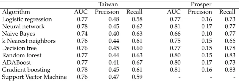
The Area Under the Curve has been used as the primary performance indicator. The measure ranges from 0.0 to 1.0, with the latter being a perfect predictor. A value of 0.5 indicates that a model performs equal to one that classifies by random guesses. Table 1 shows which algorithms have been used and what the corresponding per-formance is. Aside from the AUC, the precision and recall are also shown.

TABLE1: Performance of the different algorithms when trained and validated on the original data set.

Taiwan Prosper

Algorithm AUC Precision Recall AUC Precision Recall

Logistic regression 0.77 0.48 0.58 0.77 0.16 0.73

Neural network 0.78 0.45 0.62 0.81 0.17 0.77

Naive Bayes 0.74 0.40 0.63 0.66 0.10 0.77

k Nearest neighbors 0.76 0.44 0.61 0.75 0.15 0.66

Decision tree 0.76 0.45 0.60 0.77 0.15 0.78

Random forest 0.77 0.44 0.63 0.80 0.15 0.83

ADABoost 0.77 0.41 0.67 0.80 0.17 0.73

Gradient boosting 0.78 0.45 0.61 0.81 0.16 0.83

Support Vector Machine 0.76 0.47 0.59 - -

[image:3.595.90.485.583.719.2]

(4)

algorithm, the performances are so close together that it is difficult to draw conclu-sions based solely on the AUC. The performances achieved with the Prosper data set show more variation. Naive Bayes again has the lowest performance. The highest performance is achieved by the same two algorithms, Neural Network and Gradient Boosting. When one takes the explainability into account, the view on which of the algorithms is most suitable changes. For the Taiwan data set, the Decision Tree has a decent AUC which is 0.02 below the highest value, in the Prosper data set it is 0.04 below the highest value. Clearly a choice between explainability and performance has to be made.

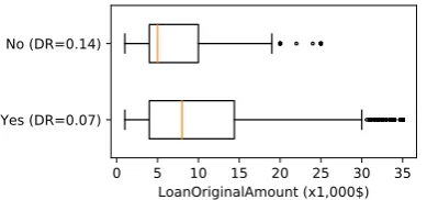
For the Prosper data set, it is interesting to see how good the models are in pre-dicting which loans don’t go into default. The best algorithms, Random Forest and Gradient Boosting, have a negative predictive value of 97,9% and even the worst algorithm, Naive Bayes, has 95,9%. This makes it interesting to use the algorithms not as default predictors, but to define a group of low risk loans.

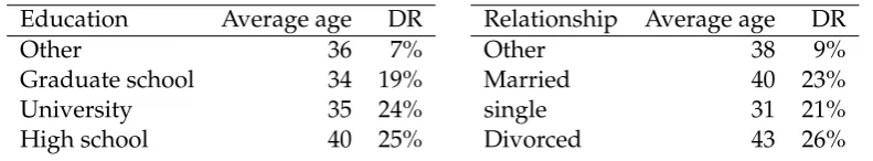
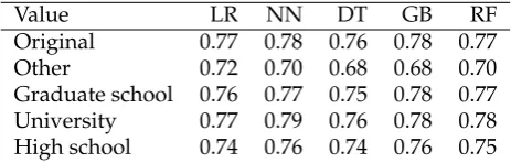
Finally, both of the data sets have been split according to certain characteristics. The goal of such a modification is to find differences in performances on specific parts of the data set. With the Taiwan data set a positive effect was observed in two occasions. Some algorithms with the Prosper data set showed an increase up to 0.03. However, with both data sets a decrease in performance was observed in most situations. The last modification was winsorization of the numerical features. This led to no substantial changes.

Based on the above mentioned findings the following conclusions are drawn. Both Gradient Boosting and Neural Network seem to be the best performing algo-rithms. They both have the highest AUC for both of the data sets. The disadvantages of those algorithms is that they tend to become a black box , making it difficult to explain why a classification is made. Furthermore, an increase in performance can be achieved by splitting the data sets by some characteristics, but this should be examined case-by-case.

Resampling

The data sets used in this research project where imbalanced. The Taiwan data set had 22% of the samples in the minority class, the Prosper data set even less, only 8%. To remove the imbalance the following methods have been used: random un-dersampling, random oversampling, SMOTE (regular, borderline1 and borderline2) and ADASYN (2, 5 and 10 neighbors).

(5)

Preface

I proudly present you my master’s thesis, which is the result of more than half a year of research. This thesis is written in order to graduate from the master Industrial Engineering and Management at the University of Twente. Meaning that this thesis marks the end of my life as a student, after seven years, which feel more like three of four.

The majority of this thesis has been written during my internship at Accenture. During this time I have been able to get to know Accenture and some of its peo-ple. From whom I appreciate their willingness to discuss the dry matter of machine learning while enjoying a cup of coffee. I want to especially thank my external su-pervisor, Paul Weiss, for the opportunity to write my thesis at Accenture which gave me the possibility to get to know the company from within and for his advice and comments on my thesis.

I also thank my supervisors from the university, Toon de Bakker and Mannes Poel for guiding me through the process of writing a thesis. Your advice and com-ments on my research were most useful and helped me to create the result you are reading now.

My parents have supported me throughout all my years as a student, for which I am most grateful and want to thank them. I also thank all my friends I met during my study in Enschede, for all the good times we had and will have in the future. Finally, I want to thank my girlfriend for her support and patience. Even when too much time went into writing my thesis.

Amsterdam, June 2018

(6)

(7)

Introduction

In this chapter the research is introduced to the reader. First Accenture is introduced, the company where this research project is performed. This is followed by a descrip-tion of the project context, after which the problem is described and the research objective is given. Based on the research objective several questions are defined to which this research project will give an answer. Finally, this chapter is concluded with an outline of the rest of the report.

1.1 Organization

Accenture is a global management consulting firm with over 400,000 employees. The history of the company goes back to 1953, but it has been working under its own name since 1989 as Andersen Consulting. Since 2001 the current name, Accenture, is used. In that same year the company had its initial public offering at the New York Stock Exchange.

The company has divided its business into several categories: strategy, consult-ing, digital, technology and operations. This research project is carried out within the consulting branch and more specific the banking industry. This department is specialized in supporting banks with a broad range of services. To stay up to date with new technologies there is large interest in research focused at financial innova-tions.

1.2 Project context

(10)

financial institutions are always working on methods to improve their possibility to estimate risk.

Turing (1950) explored the topic of computing intelligence. In his article, he asked the question “can machines think?”, by asking that question he was years ahead of his time. The term machine learning was first used in Samuel (1959) about learning a machine to play checkers. It took until the 90’s before machine learn-ing started to flourish as its own field of research (Langley, 1995). This came with a shift of paradigm: from achieving artificial intelligence towards tackling practical and solvable problems. Since then machine learning has slowly evolved into a more mature technology. In 2015 several tech giants open-sourced their machine learning tools, among which where Microsoft, Facebook and Google (Thomas, 2015; Chin-tala, 2015; Dean, 2015). With the widespread availability of tools, enterprises across industries start to experiment with machine learning. To be able to implement ma-chine learning, it is necessary to have a thorough understanding of the available algorithms. Knowing which algorithm is most suitable for a task is a part of that understanding.

1.3 Problem description

As mentioned before, estimating the risk of a loan is an important task within bank-ing. This makes it interesting to research the possible improvements that can be reached by applying machine learning. Several scientific papers have been written about the expected benefits of using machine learning in default prediction (Abellán and Mantas, 2014; Harris, 2015; Huang, Chen, and Wang, 2007). These show that machine learning can lead to a higher in accuracy default prediction, compared to conventional methods. However, most of these papers are limited in the number of algorithms compared. Moreover, the observation is that nearly all papers use a different data set, making the results difficult to compare. This creates an interest-ing opportunity to determine the performance of a broad range of algorithms on the same data sets.

1.4 Research objective

Now that the problem has been described, an objective for this research project is defined. The objective is to develop knowledge about the predictive performance of different machine learning algorithms when used to predict defaults in loans. This is done by implementing different machine learning algorithms which can be used to classify samples. These different algorithms will be used to predict the defaults on loans. The loans come from two data sets with loans of which it is known whether or not they went into default. The final part of the objective is to compare the per-formance of the used algorithms and to determine which is most suitable for this task.

(11)

1.4.1 Main question

The main question of this thesis is defined as:

What is the predictive performance of machine learning when applied to the prediction of defaults in loans?

1.4.2 Sub questions

Which machine learning algorithms are suitable for making binary classifica-tions?

The first step of this research project is to determine what types of machine learning and which algorithms exist. Based on the findings from that analysis a selection of algorithms has to be made that will be used in this research project. This question will be answered using relevant literature.

What criteria should be used to objectively and accurately measure the perfor-mance of different machine learning algorithms?

The goal of this research project is to make a comparison of the performance of dif-ferent machine learning algorithms. To be able to do so in a objective way, it is necessary to accurately measure the predictive performance. The measure that will be used in the experiments is based on a literature review.

What is the performance of the different machine learning algorithms when used to predict defaults?

The final subquestion is to actually determine the performance of the different gorithms. The answers of the previous questions are required to configure the al-gorithms and prepare the data. This answer will be answered by implementing the algorithms and using them in combination with the prepared data sets.

1.5 Report outline

(12)

(13)

Chapter 2

Theoretical framework

The theoretical framework contains the necessary background to answer the re-search questions defined in the previous chapter. The chapter starts with a section about relevant research on the same topic, to provide a context for this thesis. A brief description of credit scoring will be given next. This subject is followed by a section about machine learning and goes in depth about the different forms of ma-chine learning. This is followed by a section on the impact of an imbalance between classes in data sets, after which several performance measures are treated. To get to a reliable performance measure, cross-validation is required. It is therefore the next topic. After cross-validation it will be discussed how several models can be com-bined into so-called ensemble models. Finally the different algorithms used in this research project will be discussed in detail.

2.1 Current state of the literature

In this section of the Theoretical Framework some relevant literature will be de-scribed. The goal is to make the purpose and added value of this research project clear.

To find the beginning of artificial intelligence in scientific literature, one has to go back to 1950, the year in which Turing (1950) wrote his paper Computing Machinery and Intelligence. Since then, and particularly in recent years, the topic has gotten a lot of attention. According to Jordan and Mitchell (2015) machine learning has become the technology of choice within artificial intelligence to achieve practical so-lutions. They mention the rapid decrease in the cost of computational power and the availability of online data as two factors that have driven the rapid development of machine learning. As an important financial application of machine learning Jordan and Mitchell mention the detection of credit-card fraud. Their paper is concluded by mentioning it is necessary that society begins to consider how to maximize the benefits of machine learning.

This research project is not the first about using machine learning to predict de-faults in loans. Using machine learning to score credit has been done since before 2000, for example Langley (1995) already mentioned it as a possible use case for machine learning. Since then a lot has happened in the field of machine learning, among other reasons due to the increasing computational power. In more recent years multiple scholars have performed research into the accuracy of machine learn-ing when used for default prediction. However, most often the research is about a single new algorithm which is compared to a few benchmarks.

(14)

and Wang, 2007). These projects show that machine learning can lead to a high ac-curacy in credit scoring. However most of these projects are limited in the number of models compared and are based on different data sets which make the results in-comparable. One of the early papers in which machine learning is applied to default prediction is about Support Vector Machines (Shin, Lee, and Kim, 2005), but no com-parison is made. Alaraj, Abbod, and Hunaiti (2014) use a nearal network to make default prediction, but again no comparison is made with other techniques. Khan-dani, Kim, and Lo (2010) use machine learning to make default predictions and do make a comparison. However this is only between three algorithms, where in this research project a more broad comparison will be made.

Now that machine learning is slowly becoming a more mature technology that is starting to be used in practice another type of research is needed. Before making the choice on which algorithm should be implemented it is required to make a broad comparison between algorithms. For this comparison it is important that the same data set is used, otherwise the results cannot be compared.

Only summing up research projects with a positive conclusion would give a bi-ased expectation of this project. Recently some critical reports have been published. According to a report by Gartner (2016) machine learning is currently on the top of a hype cycle and thus too high expectations exist. When a technology passes the top of the hype cycle, expectations will drop considerably. If machine learning moves to through the hype cycle as expected, it will get mainstream adoption in two to five years.

2.2 Credit risk

As mentioned before the goal of this research project is to determine if machine learning can be used to make better loan decisions. The reason for chasing this goal is to minimize the credit risk the bank is exposed to.

Credit risk arises from the possibility that borrowers, bond issuers, and counter parties in derivatives transactions may default (Hull, 2015).

In this project the focus is on the credit risk that arises from the possible defaults of borrowers. The formula for the expected loss from defaults is given in Equation

(2.1). EADis the expected exposure at the time of default,LGD is the fraction lost

given default andPDis the probability of default.

∑

i

EADi×LGDi×PDi (2.1)

When the customer of a bank is unable to repay a loan, it goes into default. The goal of the bank in such a situation is damage mitigation, it will try to minimize the amount that has to be written off due to the default. When accepting a customer for a loan the risk is determined. Part of this process is determining the expected amount that has to be written off, if the loan goes into default. The expected fraction that has to be written off, is the loss given default.

2.3 Machine learning

(15)

learn and make predictions based on data and feedback. An important characteristic of machine learning is that it is not explicitly programmed to follow certain decision rules to create results. Instead it has the capability of creating those rules based on data and feedback.

A computer program is said to learn from experience E with respect to some class of tasks T and performance measure P, if its performance at tasks in T, as measured by P, improves with experience E (Mitchell, 1997).

By applying this definition to the goal of credit scoring it figures that information about historical loans and their default status is required to train a model into learn-ing to predict defaults.

2.3.1 Features

In machine learning, a feature is a single measurable property of the phenomenon that is being studied. All the features describing a single entry usually form the feature vector. Features have one of the four following data types.

– Nominalfeatures are labels without any quantitative value and the labels do not

have a specific order. Examples of such a feature are gender or color.

– Ordinalfeatures are labels without a quantitative value but with a specific order.

An example is satisfaction (unhappy, neutral, happy).

– Interval features are numeric values of which the order is known and also the

difference between the values. An example of such a label is the Celsius scale, the difference between the values is known. The problem with interval scales is that

they do not have a true zero. This makes it impossible to calculate ratios, 10◦_{C is}

not twice as warm as 5◦_C.

– Ratio features are similar to interval features but in addition have an absolute

zero. This makes it possible to multiply and divide the values. Weight and length are examples of ratio features.

2.3.2 Learning methods

Machine learning problems are subdivided into different categories. The most used method of categorizing machine learning tasks is by learning method. In this sec-tion, the most used learning methods are described. Each category has a textual description, an example and a mathematical representation.

Supervised learning

The first method is supervised learning, this method is used when there is an input and a known output and the task is to learn the mapping form input to output (Al-paydın, 2010). This task can be described as to infer a function from label training data, which can be used to classify future unlabeled data.

(16)

infer a function relating the features to the car being a family car or not. The goal of inferring this function is to determine for future cars whether the car is a family car or not.

Given a set S, containing N training samples, s, {(x1,y1), ...,(xN,yN)} with xi

being the feature vector of thei-th example andyibeing the corresponding label, the

goal is to determine a functiong: X→Y. gis a function that maps the input space

X(the features) to the output spaceY(the labels). The performance of the function

gis crucial in the performance of the machine learning model. It is usually assumed

that the values in a feature vector xi, are generated randomly and independently

according to a fixed and unknown random distribution (Maimon and Rokach, 2005).

Semi-supervised learning

Semi-supervised learning considers the problem of classification when only a small subset of the observations have corresponding class labels (Kingma et al., 2014). Such a learning algorithm lies between supervised learning and unsupervised learn-ing, the latter of which is discussed later in this section. At first it might seem strange that unlabeled data has any use and one might expect to discard the unlabeled data and regard the task as if being supervised learning. In Figure 2.1, the left image shows a situation with four labeled data points, the line shows a classifying border that is a good fit. The right image shows the same data points, but now unlabeled data is added. By analyzing the newly added unlabeled data, a pattern arises in the data. This pattern is only visible by taking the unlabeled data into account.

FIGURE2.1: Graphs showing the possible added value of unlabeled

data.

(A) Classification boundary based on

labeled data only.

2 4 6 8 10

x y

(B) Classification boundary based on

labeled and unlabeled data.

2 4 6 8 10

x y

Situations in which semi-supervised learning is practical, usually have a high cost of determining labels in the training set. An example of such a situation is image recognition in which lots of data is available but adding labels is manual work and thus expensive.

The following notations are based on Zhu, Ghahramani, and Lafferty (2003). In

semi-supervised learningllabeled points are given,(X_l,Y_l) = _{(x1,y1), ...,(xl,yl)},

anduunlabeled points are given,Xu={xl+1, ...,xl+u}. In semi-supervised learning,

on usually hasl u. Due to the complexity of semi-supervised learning further

details are limited to the general idea. Which is to find functions f : V _→ R, with

(17)

functionsf must agree with the labeled dataXl and should be smooth regarding the

unlabeled dataXu.

Reinforcement learning

A learning algorithm that works by means of reinforcement does not receive any la-bels at first. Such a system learns by interacting with its environment by producing actions which affect the environment. The effect on the environment returns a re-ward or punishment. The goal of the algorithm is to produce actions in such a way that the reward is maximized or the punishment is minimized.

In recent times attention has been going out to cars autonomously driving a route. Learning a car to traverse such a route without violating any laws or caus-ing accidents can be done by applycaus-ing reinforcement learncaus-ing. For example, an al-gorithm in a simulated environment must learn how to drive a car along a certain route without violating any traffic rules. At first the algorithm will simply perform random actions, by punishing traffic violations the algorithm will start to learn how to drive according to the rules. By repeating this process for many runs and reward-ing the algorithm for reachreward-ing the end of the route it will slowly start to learn how to safely drive a car.

The notations used in this explanation are based on Maimon and Cohen (2009). Reinforcement learning is usually based on the Markov Decision Process, or MDP.

Such a process contains all possible statesS, actionsA, rewardsRand state-transitions

P. State-transitions specify the resulting state of applying a certain action to the

cur-rent state. The sets of states and actions can theoretically be both finite and infinite.

The learning algorithm starts at time t in a certain environmentst ∈ S and reacts

by selecting an actionat ∈ A. This leads to the algorithm getting a rewardrt

deter-mined by the reward functionR(st,at). The result of selecting an action is a

tran-sition of the environment to a statest+1 with probability P(st,at,st+1)determined

by the state-transition function. The algorithm starts performing actions within this MDP without knowing anything about the reward function or the state-transition function. The goal of the algorithm is to find a policy that maximizes the achieved reward within the MDP.

Unsupervised learning

The last learning method discussed is unsupervised learning. In this method, the algorithm is trained using just an input set, no output, desired results or feedback is given. The algorithm must find structure in the data by itself. Unsupervised learning can be seen as finding patterns in data that are different from pure unstructured noise (Ghahramani, 2004).

A promising use of unsupervised learning is in the behavior-based detection of network security (Engel, 2017). Due to the amount of data generated it is impossible for a human to analyze all the data. An algorithm based on unsupervised learning could detect anomalies in the data without being learned what a breach looks like. When such an anomaly is detected, IT security could be notified.

2.3.3 Weak and strong learners

(18)

slightly better than random guessing (Freund and Schapire, 1997). Strong learners are all more complicated models.

2.4 Working with imbalanced data sets

In real-world data sets the number of ’interesting cases’ is often small in comparison to the total number of instances. Consider for example a data set with loans and defaults, since in normal situations a small fraction of loans go into default the data set is imbalanced. This causes problems in training and evaluating machine learning models. Machine learning models can be evaluated by their predictive accuracy. In imbalanced data sets this measure is often misleading. Consider a data set with 99% of non-interesting (negative) instances, a model that classifies nothing as interesting (positive) will have a predictive accuracy of 99%. This accuracy is useless since it is unable to find any interesting case. Such a result is often seen with imbalanced data sets because the set contains too few interesting cases for the model to learn their characteristics. A method to mitigate this problem that received ample attention is over and under-sampling (Chawla, Japkowicz, and Kotcz, 2004).

2.4.1 Over-sampling by replication and under-sampling

The most simple and straightforward method to balance imbalanced data sets is by using over-sampling by replication or under-sampling. The first of these is simply to replicate random samples of the under represented case until the data set is bal-anced. This results in a data set with multiple identical samples which might lead to specific and small decision regions which may cause over-fitting. Under-sampling is a method to balance the data set by ignoring a certain part of the over represented class. The issue with this method is that it leads to a loss of information and might cause under-fitting. It also decreases the size of the data set, which might result in a too small data set to still be able to train an algorithm.

2.4.2 Synthetic minority over-sampling technique

In the previous section, over-sampling by use of replication and under-sampling were introduced. Since that method replicates existing cases, the model trains on more but identical positive cases, this can cause over-fitting. To counter this issue Chawla et al. (2002) developed a technique to generate synthetic samples: synthetic minority over-sampling technique (SMOTE). Using synthetic samples, the classifier creates a larger and less specific decision area, this leads to better generalization of the decisions. Blagus and Lusa (2013) found that SMOTE does not always perform well on high dimensional data sets.

The method works by selecting the k nearest neighbors for each sample in the

under represented class. Synthetic samples are generated on the line segments con-necting neighbors. New samples are generated by calculating the difference between the feature vectors of a base sample and a neighbor. This difference is multiplied by a random number between 0 and 1, and is added to the feature vector of the base sample. The resulting vector is the feature vector of a newly generated sample. De-pending on the required amount of over-sampling, neighbors are selected randomly

from thek nearest neighbors. A graphical representation of the SMOTE process is

(19)

FIGURE 2.2: (a) The original distribution of data. (b) The

border-line minority samples. (c) The borderborder-line synthetic minority samples (Han, Wang, and Mao, 2005).

Borderline-SMOTE

Han, Wang, and Mao (2005) propose two alternatives on SMOTE in which only sam-ples near the border between classes are over-sampled. They show that their pro-posed methods achieve a higher true positive rate and F-value. The philosophy of focusing on the borderline is that samples near the border are more apt to be mis-classified and thus should get more attention.

The first proposed alternative is borderline-SMOTE1, it works as follows.

As-sume a set,S, is given containing training samples,si = (xi,yi), with xi being the

feature vector of thei-th sample andyi being the corresponding label. The setS is

split, positive samples are a part ofSp and negative samples ofSn. For this

expla-nation it is assumed the positive samples are under-represented. For all samples in

the minority class,Sp, theknearest neighbors are determined, these neighbors can

belong to either class. The number of samples from the majority class among the

nearest neighbors is denoted byk0_{, for which 0}_≤ _k0 _≤ _k_{. If the number of majority}

class neighbors equalsk for a sample, it is regarded as being noise. If the sample

has more neighbors in the majority class as in the minority class (k/2< k0 < k), the

sample is added to a setD(danger). The result will be a set D _⊆ S with samples

along the borderline of the classes. Finally the SMOTE algorithm is performed upon

the setDas explained in the previous section.

The other proposed method is borderline-SMOTE2. In addition to the proce-dure for borderline-SMOTE1, a synthetic sample is calculated on the line segment

between each sample inDand its nearest negative neighbor. In borderline-SMOTE1

the synthetic samples are generated by multiplying the difference between two sam-ples with a random number between 0 and 1. For borderline-SMOTE2 the difference is multiplied with a random number between 0 and 0.5. This results in a synthetic sample closer to the positive sample.

2.4.3 Adaptive synthetic sampling

(20)

for generating a synthetic sample. Resulting in a greater focus on difficult regions which should lead to better predictions.

ADASYN is started by determining the number of synthetic samples that have to

be generated,G. This is done by calculating the difference betweenNn, the number

of majority samples, andNp, the number of minority samples, as shown in Equation

2.2. It follow thatNn > Np and thusG> 0. βis a parameter to specify the desired

balance, withβ∈ [0, 1]. A value of 1 means a perfectly balanced data set.

G= Nn−Np×β (2.2)

The next step is to calculate a measure for the learning difficulty for each minority sample. This measure is based on the number of samples in its close vicinity that are

majority samples. For the calculation, theknearest neighbors are taken for

consider-ation.kis a predetermined model parameter. The number of neighbors that belong

to the majority class is denoted ask0_{. The relative learning difficulty for sample}_i_is

calculated as given in Equation 2.3. Finally the relative difficulty for each minority sample is normalized in such a way that the sum of all difficulties equals one.

ri =k0i/k (2.3)

Using the normalized difficulty measure,bri, the number of synthetic samples to

gen-erate per specific minority sample can be determined:

gi =bri×G (2.4)

The samples are generated using the same method as in SMOTE.

2.5 Model performance measures

Since the goal of this research project is to compare several methods of machine learning, it is required to define criteria on which the methods are to be compared. In this section several statistics to assess the performance are discussed.

2.5.1 Confusion matrix

The first method to analyze the performance of a classification algorithm is by us-ing a confusion matrix. It is a method to visualize the accuracy usus-ing a table, an example is shown in Table 2.1. For the purpose of explaining the confusion matrix a classifier that classifies instances as positive or negative is assumed. Four fields have to be calculated to fill in the matrix, true positive, false positive, true negative and false negative. These fields are simple to calculate. For example, true positive is the number of occurrences correctly classified as positive and false negative are the occurrences incorrectly classified as negative.

TABLE2.1: Confusion matrix of a two-class problem.

Predicted positive Predicted negative Positive (P) True positive (TP) False Negative (FN) Negative (N) False positive (FP) True Negative (TN)

(21)

positive. If the accuracy would be purely evaluated on the actual positive instances being classified as positive such an algorithm appears to be performing perfect. To prevent this situation, the confusion matrix can be used. Since the column with the negative predictions is empty, it is clear that the algorithm is not working,

2.5.2 Accuracy

Using the values calculated for the confusion matrix it is possible to calculate sev-eral interesting statistical measures. The first of which is the accuracy, shown in (2.5). The abbreviations used in this section are identical to those given in 2.1 The accu-racy is used to calculate the fraction of total predictions that is correctly classified. A random classifier will get on average half of the classifications correctly. Values above 0.5 indicate the model has a higher accuracy as random guessing. A perfect prediction has accuracy 1.0.

accuracy = TP+TN

P+N (2.5)

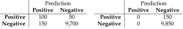
A drawback of using the accuracy to assess the performance of a classifier is the so-called accuracy paradox. This paradox states that a model with a higher accuracy may have a lower predictive power. To explain this paradox assume a situation in which insurance fraud has to be detected. Two different models are available, the performance of both models is given in Table 2.2. The model belonging to the left table detects 100 out of 150 cases of fraud and has an accuracy of:

100+9, 700

150+9, 850 =0.980

The model belonging to the right table, is not able to detect any fraudulent activity, it has no predictive power. Its accuracy is:

0+9, 850

150+9, 850 =0.985

Even though the second model has no predictive power, it has a higher accuracy. This disadvantage of accuracy is important to keep in mind when evaluating the performance of different models. To avoid this paradox several other statistics have been developed to quantify model performance.

TABLE 2.2: Two confusion matrices showing the accuracy paradox.

The right example has a higher accuracy but is a worse predictor.

Prediction Positive Negative

Positive 100 50

Negative 150 9,700

Prediction Positive Negative

Positive 0 150

Negative 0 9,850

2.5.3 Precision and recall

Precision, or positive predictive value, is the fraction of positive classified instances that is true positive.

Precision = TP

[image:21.595.128.448.597.649.2]

(22)

Recall, also called sensitivity or true positive rate, is the fraction of true positive instances that are classified as positive.

Recall = TP

TP+FN = TP

P (2.7)

These two statistics are usually used together. Either both are given, or the

statis-tics are combined in a different statisstatis-tics, for example theF1-score which is discussed

later in this chapter.

2.5.4 F1-score

As mentioned in the previous section, precision and recall are often combined. One

of the statistics resulting from such a combination is theF1-score. As can be seen in

Equation 2.8, theF1-score is equal to the harmonic mean of the recall and precision.

A disadvantage of theF1-score is that it does not take the true negatives into account.

F1-score= ₁ 2

precision+ recall1

=2× precision_precision×₊recall_recall (2.8)

2.5.5 Area under the curve

To understand the details of the area under the curve, it is required to first explain the receiver operating characteristics (ROC) curve. It is used for visualizing classifier performance and has long been used in signal detection theory to depict the trade off between true and false positive rates of classifiers (Fawcett, 2006).

An ROC curve is created by plotting the true positive rate (TP/P) against the

false positive rate (FP/N) for different thresholds. Since classifiers calculate a score

between 0.0 and 1.0, a threshold has to be chosen as border between positive and

negative classifications. The calculated score,x, can be can be seen as being sampled

from a continuous random distribution X. An instance is classified as positive if

x> T, with T being the chosen threshold. Different thresholds will result in different

true and false positive rates.

Figure 2.3 shows three examples of an ROC curve: a random model and two models with predictive capabilities. The ROC curve of a random model approaches

the line stretching from(0, 0)to (0, 1). The reason behind this behavior is best

ex-plained with an example. Assume that a random fractionKis classified as positive,

then a fractionKof the instances that should be classified as positive will be correctly

classified, and the same fractionKof values that should be negative will be correctly

classified as negative. For models that perform better than random guessing, the true positive rate will be higher than the false positive rate and thus the model will have a ROC curve above the diagonal.

Thearea under the curve, AUC, is a measure that tries to summarize the ROC

(23)

FIGURE 2.3: Graph containing the ROC of a random classifier and

two better performing classifiers.

0.2 0.4 0.6 0.8 1

Random model Model A Model B

2.6 Cross-validation

When training models to make predictions, it is needed to have a method for esti-mating how accurately the model will make predictions in practice. In cross-validation the data is split in a set used to train the model, the training set, and a set against which the models is tested, the test set. Many types of cross-validation rely on mul-tiple iterations to reduce variability. In the following sections several methods are discussed.

2.6.1 Holdout method

The holdout method randomly splits the data set into two sets,d0 andd1, the

train-ing set and test set, respectively. The model is trained ustrain-ingd0and validated using

d1. Usually a majority of the samples is assigned tod0. Typical splits in data

min-ing applications range from 30:70 to 10:90 (Zhang, 2009). The disadvantage of this method is the usage of a single train/test split, this makes the method susceptible to random variations.

2.6.2 Repeated random sub-sampling validation

This method works by repeating the holdout method. Because of this repetition, it is also known as Monte Carlo cross-validation. In each replication the data set is randomly split into a training and test set. The results are averaged over all itera-tions. The disadvantage of this method is that some samples may never be used as validation whereas other may be selected multiple times.

2.6.3 k-fold cross-validation

Ink-fold cross-validation the data set is shuffled and split intok equally sized sub

sets. Of theseksets, a single set is retained to be used as test set, the remainingk–1

sets are used as training set. This process is repeatedk times, with each of the sub

sets being used as test set once. The performance is averaged over all iterations to get an accurate estimation of model performance. Rodríguez, Pérez, and Lozano

(2010) used a sensitivity analysis to determine thatkshould usually be 5 or 10 when

(24)

2.7 Ensemble models

The basic idea of ensemble models is to combine several individual classifiers into a single composite classifier (Rokach, 2009). The goal of creating such a composite classifier is to obtain a model performing better than would be possible with a sin-gle classifier. Rokach (2009) has determined four factors to describe the differences between ensemble models.

– Ensemble size- The number of classifiers in the ensemble.

– Combining method- In an ensemble model each classifier makes a prediction. To

come to a final classification the separate results have to be combined according to a certain method.

– Diversity generator- Combining classifiers into an ensemble only has an effect if

the individual classifiers are not identical. Most methods to create diversity are based on differences in input data or differences in model design.

– inter-classifiers relationship- Ensemble models can be divided in sequential and

concurrent models based on whether the individual models influence each other.

Several ensemble models are described in Section 2.8.

2.7.1 Combining method

The most simple form of combining classification is hard voting. This method allows each classifier to cast one vote, it assigns the instance to the class which received most votes (Ali and Pazzani, 1996). In case of a draw the instance is assigned randomly to one of the classes with the most votes.

In soft voting the individual classifiers all determine the probabilities of the in-stance belonging to each class. These probabilities are summed for each class and the instance is assigned to the highest probability class. This method limits the clas-sifiers in the ensemble to those that base classifications on a probability.

2.7.2 Diversity generator

Diversity in an ensemble model can be generated in several ways. The first approach is to train each of the models in the ensemble on a different part of the data set. In most of these approaches the data is separated randomly, but other more structured approaches exist. Another approach is to use different algorithms, this method can be combined with randomly selected data. Many algorithms are used, for example one that changes the weight of the samples at each iteration based on the difficulty the algorithm has with classifying that sample.

2.7.3 Inter-classifiers relationship

(25)

The other group consists of the sequential ensemble models, these all have some kind of interaction between individual classifiers. An important group of sequential models comes in the form of boosting models. These models work by repeatedly training a weak learner on various selections of training data. The data selection is based on the results of previously trained weak learners. After reaching a prede-termined stop criterion all weak learners are grouped and can be used to make a classification.

2.8 Model descriptions

In this section several machine learning algorithms are discussed. Of these algo-rithms a description will be given in combination with a mathematical formulation.

2.8.1 Logistic Regression

The first of the machine learning algorithms discussed, is Logistic Regression. It has been proposed by Cox (1958), making it one of the older machine learning algo-rithms. The primary idea of Logistic Regression is to use techniques developed for linear regression to model the probability of a sample belonging to a certain class. This is done using a linear predictor function, Equation 2.9, which is a linear

combi-nation ofmfeature values andm+1 regression coefficients.

f(i) =β0+

m

∑

i=1

βixi (2.9)

Logistic regression is different from other forms of regression due to the way the linear predictor is linked to the probability of a certain outcome. It transforms the output of the linear predictor using the logit function, depicted in Figure 2.4, which is the natural log of the odds. An advantage of using the logit function, is that it takes any real value as input and returns a value between zero and one.

logit(p) =ln

p

i

1−pi

= f(i) (2.10)

FIGURE2.4: The standard logistic function.

−6 ₋4 −2 0 2 4 6

0 0.5 1

Using the above transformation of the linear predictor, the following equation for the probability of a positive sample can be determined.

p(x) = (1+eβ0+∑mi=1βixi₎−1 _(2.11)

(26)

equation to determine the coefficients. Instead other methods like maximum likeli-hood estimation are used. In this method an iterative process is used during which in each iteration the coefficients are slightly changed to try to improve the maximum likelihood. In this research project two methods to fit the model are taken in to ac-count. These methods will not be discussed in depth since it is not within the scope of this research project. The first method is Liblinear, it used a coordinate descent al-gorithm to find suitable values for the coefficients. The second method is saga which uses a stochastic average gradient descend. The second method usually is faster on large data sets.

In the loss function that is minimized it is usual to include a regularization term. Such a term is to penalize complex models and favor models which are simpler. With Logistic Regression two types of regularization are commonly used, L1 and L2. The first of these is a regularization that favors sparse models, or models where a large fraction of the coefficients is zero. L2 is used as regularization term when a sparse model is not suitable. When the data set contains highly correlated features, L1 should be used as regularization term. It picks a single of the correlated features and sets the coefficient of the other features to zero. L2 would simply shrink the coefficient of all correlated features. Usually a parameters is added to the algorithm which can be used to determine the strength of the regularization.

2.8.2 kNearest Neighbors

Nearest Neighbors classification is a method that bases a classification on thek

sam-ples closest to the instance that has to be classified (Larose, 2005). This algorithm does not attempt to induce a model, it simply stores instances of the training data, making it a so-called lazy algorithm.

The basic Nearest Neighbors classification uses the same weight for each of the

kselected neighbors. In some situations it might be better to differ the weight of the

neighbors based on the distance to the sample that has to be classified. Meaning the weight will be inverse to the distance, so the closest samples will get the greatest weight.

Brute-force

The most basic computation method for the Nearest Neighbor classification is brute-force. This algorithm simply calculates the distances between all points in the data set and uses those to determine which points are closest. For small sample sizes this algorithm can return accurate result. Due to its naive nature, brute-force quickly becomes an unfeasible approach when sample size increases.

k-dtree

To counter the issue of the brute-force method being unfeasible for larger sample sizes, a more efficient method has been developed by Bentley (1975). This method used a decision tree to efficiently store distance information requiring less

computa-tions. Assume three pointsA,BandC, of these pointsAandBare very distant and

CandBare close. From this information it follows that pointsAandCare also very

distant.

Ak-dtree is constructed by iterating over several steps. In each iteration a (not

(27)

The median value of the selected feature is calculated, values larger than this median are separated from the smaller values. Now two branches have been created, each with approximately half of the samples. On both branches these steps are repeated. This process continues until the number of samples in a branch drops below a certain threshold. An example of the result of this process is shown in Figure 2.5.

After a tree has been generated, the approximately closest neighbors can easily be determined. All nodes of the tree are applied on the new instance, the branch where the new instance ends up in, contains samples that are close. For all of these samples the distance to the new instance is calculated to find nearest ones.

FIGURE2.5: Schematic overview of ak-dtree.

Ball tree

In high dimensional space it becomes computationally expensive to create ak-dtree.

In those situations it is computationally favorable to create a ball tree (Bhatia, 2010). Omohundro (1989) describe a ball tree as a binary tree of which each node represents a hypersphere called a ball. Each node of the tree splits the data into two disjoint sets, each set is contained by the smallest ball containing all points. The hyperspheres are allowed to cross, data points are assigned to the sphere of which the center is closest.

2.8.3 Naive Bayes

The Naive Bayes classifier is based on statistical theory, more specific on Bayes’ the-orem, Equation 2.12. Using Bayes’ it is possible to calculate the probability that a certain hypothesis is true given observed evidence. The naive part comes from the fact that in Naive Bayes, it is assumed that all of the features are independent from each other.

P(A|B) = P(B|A)P(A)

P(B) (2.12)

(28)

P(U|+) = P(+|U)P(U) P(+)

P(U|+) = P(+|U)P(U)

P(NU)P(+_|NU) +P(U)P(+_|U)

P(U|+) = 0.99×0.005

0.995_×0.01+0.005_×0.99 =33.2%

The above calculations show that the aforementioned probability equals 33.2%. Even though the intuitive answer would be 99%.

Since Bayes’ theorem can be used to calculate the probability that something is true given evidence, it can be used to calculate the probability that a new sample belongs to a certain class given the evidence. Classification is done by calculating the probability that the sample belongs to a class, for each class. The sample is assigned

to the class with the highest probability. In the above example P(U_|+) = 33.2%

soP(NU|+) = 66.8%, therefore the drug tested person is assigned to the ’no drug

user’ class. In the calculations for the different classes the evidence, or sample, is identical, therefore it is possible to discard the denominator of Bayes’ theorem and still make the same classification.

2.8.4 Decision Tree

A Decision Tree probably is one of the best known classifiers due to its logic struc-ture. Decision Tree classifiers are extensively described by Rokach and Maimon (2009). A Decision Tree consists of connected nodes which form a rooted tree, mean-ing that the tree has a smean-ingle root node as startmean-ing point. All followmean-ing nodes have a single incoming edge, if the node also has outgoing edges it is called an internal node. Each of the internal nodes splits the data set according to a certain logic. In classification this split is usually based on the value of a certain feature. Nodes that do have incoming edges but no outgoing edged are called leaves. Leaves are as-signed to a label based on which label is most appropriate. After a tree has been constructed, the classification is done by starting at the root node and following through the internal nodes until a leave has been reached

Constructing an optimal Decision Tree is only feasible for small problems due to computational requirements (Hancock et al., 1996). This results in the need for heuristic algorithms. In this research the CART algorithm will be used. A Decision

Tree is trained on a feature set containing X = xi, ...,xn and corresponding labels

Y = yi, ...,yn. At each nodemthe relevant part of the set is represented byQm. The

construction algorithm tries to find a splitθ = (j,tm), with featurejand thresholdtm,

that splitsQintoQle f t(θ)andQright(θ)with a minimized impurity. Several measures

can be used to calaculate the impurity of which Gini and Entropy are widely used.

Equation 2.13 shows how the Gini is calculated, pmk is the probability of a sample

(29)

pmk= _N1

m _i_∈

∑

_R_mI(yi = k) H(Xm) =

∑

k

p_mk(1₋p_mk) (2.13)

By combining the weighted impurity ofQle f t andQright a measure for the split is

constructed, Equation 2.14. The goal is to findθ∗that minimizes this measure.

G(Qm,θ) = n_Nle f t

m H(Qle f t(θ)) + nright

Nm H(Qright(θ)) (2.14)

This process is executed in a recursive manner. After each iteration the process is

repeated forQle f tandQrightuntil a stop criterion is reached. This criterion can be a

maximum depth or a minimum number of remaining samples.

2.8.5 Artificial Neural Network

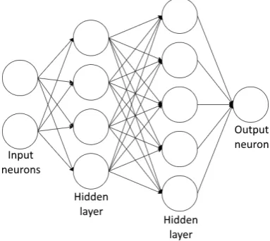
An Artificial Neural Network is is a network of interconnected neurons. This sec-tion is based on Zhang (2009). Each neuron receives an input, processes these signals and produces an output signal. A Neural Network consists of several layers of neu-rons, see Figure 2.6 for a schematic overview. The leftmost layer consists of the input neurons, the rightmost neurons are the output neurons. The layers in between are called hidden layers. The neurons are connected in such a way that the output of one neuron is the input of all neurons in the next layer. The exceptions are the input and output neurons. Input neurons have no predecessor and are used as input for the network. Output neurons have no successor and function as network output. In classification problems with two classes only a single output neuron is used. De-pending on the value of the output neuron the sample is assigned to either class. When more then two classes exist, each class has a corresponding output neuron and the sample is assigned to the output neuron with the highest value.

[image:29.595.222.353.105.156.2]

FIGURE2.6: Schematic overview of a Neural Network.

Figure 2.7 shows a schematic overview of how an artificial neurons operates. A

neuron receives inputsxijwith weightswij. Withibeing the neuron from which the

signal is the output andjthe neuron which receives the signal as input. The input

[image:29.595.190.382.531.702.2]

(30)

are usually given as a matrixWl, containing all weights for layerl. The weights are

changed repeatedly during the training process and do not have to sum to 1.

pj =

∑

i

wijxij (2.15)

Since a neuron has to output a signal, the next step is to transform the calculated input using a transformation function. Such a function can be of any form, but most used are logistic sigmoid, hyperbolic tangent or rectified linear unit (Schmidhuber, 2015).

FIGURE2.7: Schematic overview of a

sin-gle artificial neuron.

FIGURE 2.8: Three different activation

functions.

−4 −3 −2 −1 1 2 3 4

−1 −0.5 0.5 1

pj oj

Sigmoid Hyperbolic ReLU

The equation of the logistic sigmoid is given as Equation 2.16 and drawn in Fig-ure 2.8 as a black line. The function has a minimum value of 0 and a maximum of 1. The equation of the logistic sigmoid is shown below. An advantage of using the sigmoid as activation function is its bounded nature. This causes the network itself

to be bounded, if pj 1, the transformation function will never result in a value

higher than 1. In many cases this is a desirable characteristic, because it prevents a single neuron from dominating the network. However, it also has a disadvantage,

all input values have to be normalized (µ=0,σ= 1) in order to have a meaningful

impact on the output.

f(x) = 1

1+e−x (2.16)

The second transformation function is the hyperbolic tangent, it is drawn as the red line in Figure 2.8 according to Equation 2.17. The hyperbolic tangent has a shape similar to the logistic sigmoid. The biggest difference are the bounds, where the lo-gistic sigmoid returns values between 0 and 1, the hyperbolic tangent returns values between -1 and 1. Due to its bounds it also requires input values to be normalized. The two advantages of using the tangent over the logistic sigmoid arise from its symmetry across the x-axis (LeCun et al., 1998). The first advantage is faster con-vergence in comparison with the logistic sigmoid. The second advantage is that the output will on average be closer to zero due to the possibility of negative values. Since the output of a neuron is often the input for a next neuron having an average output of zero is preferable (remember how that input data is normalized).

(31)

The last transformation function taken into account for this research is the rec-tified linear unit (ReLU). It is a function with a lot of recent attention, according to Ramachandran, Zoph, and Le (2017) it is the most used activation function as of 2017. The equation of the ReLU is given in Equation 2.18 and is graphed in blue in Figure 2.8. The ReLU has a completely different shape compared to the previous

functions, it is simply the positive part of the inputpj. This activation function was

first proposed by Hahnloser et al. (2000) based on biological motivations. According to Glorot, Bordes, and Bengio (2011), networks using the ReLU activation function outperform networks using the logistic simoid function.

f(x) =x+ ₌_max₍_0,_x) _(2.18)

As mentioned before in this section the input for the transformation is the weighted

sum of the input signalspjas shown in Equation 2.15. However, this is not

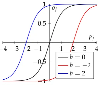
necessar-ily true in most models. Usually a biasbjis added to the input value. This bias shifts

the activation function to the left or right, as can be seen in Figure 2.9. The bias is a value that can be changed during the learning process.

oj = f(pj+bj) (2.19)

FIGURE 2.9: Impact of three different bias values on the hyperolic

tangent activation function.

−4 −3 −2 −1 1 2 3 4

−1

−0.5 0.5 1

pj oj

b=0

b=−2

b=2

Network training

Now that the components of a Neural Network are known, the mechanics to train the network have to be made clear. First a broad description of the training process is given and then the mathematical formulation is discussed.

Training a network for classification is a form of supervised learning (2.3.2), the

network is presented with samples and their known label. At first the weightswij

of the signal traveling from neuronsi to jare chosen at random. The network is

then presented with the training samples and the resulting classifications are stored. The predicted classes are compared to the real classes, the difference is expressed in some measure for the error. The first order derivative of the error with respect to the weights is calculated. Based on this derivative the weights are changed in such a way that the error decreases fastest. These steps are repeated many times until the improvement drops below a certain threshold.

[image:31.595.206.369.388.530.2]

(32)

function. For classification problems a loss function based on cross-entropy is used. Cross-entropy is commonly used to quantify the difference between probability dis-tributions. For binary distributions cross-entropy is expressed as:

−yln ˆy−(1−y)ln(1−y)ˆ (2.20)

with 0 ≤ yˆ ≤ 1 being the predicted value andy ∈ {0, 1}the real value. The

cross-entropy tends to zero when the model makes a good prediction. For example assume

y = 1 and ˆy ≈ 1, the first term, yln(y)ˆ , approaches zero and the second term,

(1−y)ln(1−y)ˆ , equals zero, thus the entropy is close to zero. The

cross-entropy also approaches zero wheny = 0 and ˆy _≈ 0. When the prediction of the

network gets less accurate, the entropy increases. Figure 2.10 shows the

cross-entropy for different values ofyand ˆy.

FIGURE2.10: Value of cross-entropy for different values ofyand ˆy.

0.2 0.4 0.6 0.8 1

2 4

ˆ

y

Cross entropy _y₌₁

y=0

The loss-function used for training a Neural Network is the average cross-entropy over all training samples including a penalty for complex models.

L= −_N1

∑

N n=1

[yln ˆy+ (1−y)ln(1−y)] +ˆ αkWk (2.21)

αkWkis a regularization term that penalizes complex models. The exact formulation

of the regularization is not within the scope of this research and not required to understand the topic. The importance given to the complexity penalty is controlled

byα > 0. The justification of penalizing complex models can be found in Occam’s

Razor. The theorem states that when having two theories with identical outcomes, the simpler one is the better.

The next step in the training process is to change the weights and biases based on the loss calculated using Equation 2.21. Updating the parameters happens according to the following equation.

wnew

i,j =woldi,j +η_δwδL

i,j (2.22)

(33)

neuron in the network transforms the input values using a predefined formula, the entire network can be expressed as a single formula using the following approach.

oj =f(pj+bj) oj =f(

∑

i

wijxij+bj)

oj =f(

∑

i

wijoj−1+bj)

oj =f(

∑

i

wijf(pj−1+bj−1) +bj)

The exact calculation of the derivative is not within the scope of this research. The derivation can be very complex and depends on the activation function. To understand the general idea of the approach is enough to keep track of the research project.

The derivative is multiplied with a factor η before being added to the weight.

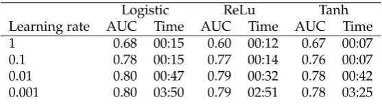
This factor is called the learning rate and determines the size of the steps when up-dating the weights. A small learning rate might cause the optimization to get stuck in a local optimum and a high learning rate can result into overshooting. Usually a value between 0.0001 and 1 is chosen.

Equation 2.22 seems to have no variables representing the biases in the network, meaning the biases will not be updated. However, using a trick it is possible to treat the biases as weights in the training process. Substituting Equation 2.15 into 2.19 results in Equation 2.23. From this it is clear that the bias can be assumed to be the weight of a signal always equaling 1.

oj = f(

∑

i

(wijxij) +bj)

oj = f(

∑

i

(wijxij) +bj×1) (2.23)

After the biases and weights have been updated the same steps are repeated. Each iteration of the training process is called an epoch. When between two epochs the loss decreases less than a certain threshold, training stops.

2.8.6 Support Vector Machines

(34)

FIGURE2.11: SVM generated maximum margin hyperplane in a two

class two dimension problem.

2 4 6 8 10

The above description clearly has a large flaw, what will happen when the sam-ples are not linearly separable? Without deviating from linearity, the solution is to add a penalty for samples on the wrong side of the separation. This penalty is mul-tiplied with a certain weight to determine the trade-off between the margin around the hyperplane and the samples on the wrong side. This weighted penalty is added to the hyperplane margin and finally minimized.

Later a more advanced method was created to separate samples using a non-linear classifier. This method is achieved by applying the so called ’kernel trick’. The general idea of the method is to map the samples to a higher dimensional space. An example showing the benefit of this transformation is shown in Figure 2.12. By

mapping data from a{x,y}space to three dimensions,{x,y,y2_}_{, it becomes possible}

to separate the two classes with a line. Each type of transformation is called a kernel, some examples are polynomial, Gaussian and hyperbolic.

FIGURE2.12: Mapping data to a higher dimension to achieve linear

separability.

(A) Two dimensional{x,y}space.

x y

(B) Two dimensions of the {x,y,y2_}

space.

x y2

2.8.7 Random Forest

(35)

training data drawn with replacement. The training procedure is similar to how a normal Decision Tree is trained except for one difference. At each split in the tree a random selection of features is selected, from which the feature for the split is selected. Usually the square root of the number of available features is used for how many features have to be drawn (Hastie, Tibshirani, and Friedman, 2009). The reason for this random feature selection is to decrease the correlation between the individual trees.

Given a feature setX= xi, ...,xnand corresponding labelsY =yi, ...,yn, for each

tree in the random forest a random subsetXr andYr is drawn with replacement.

To each of the sets of random samples a Decision Tree is fitted. At each split in the tree a random subset of features is selected on which the split can be based. For a

classification withpfeatures the most used number of features considered for a split

is√por log₂(p). This tree construction process results in Nseparate Decision Trees

which are combined in a single classifier. This can be done either by letting each classifier cast a vote or by averaging the probabilistic predictions.

2.8.8 AdaBoost

AdaBoost is a popular ensemble model developed by Freund and Schapire (1997). It is a sequential model that works by combining multiple weak learners into a strong learner. The algorithm works by adding a weak learner to the classifier in each itera-tion, until a certain criterion has been met, usually the amount of weak learners. The weak learners are trained using a weighted training set in which weights are based on the performance of the ensemble model so far. Misclassified training samples are assigned a greater weight, this weight is incorporated in the equation used to calcu-late the error of a weak learner. The result is that a greater importance is given to samples with a large weight. A weight is also given to each of the weak learners. This weight is based on the performance of the weak learner in such a way that it minimizes the training error of the ensemble model so far.

In theory an AdaBoost classifier can be constructed using any type of classifier that is able to calculate probabilities. However, AdaBoost is most often used with single level Decision Trees, called decision stumps.

A more formal definition of AdaBoost follows. The algorithm combinesTweak

learners into an ensemble. At each iteration t = 1, 2, ...,T a new weak learner is

added to the ensemble. These weak learners are trained using a set, containingm

samples, in which each sample has a weightwi. At the start of the algorithm, each

sample is given an equal weight, 1/m. The samples all have a label that is based on

the true classification, it denoted as−1 or 1. Using this training set a weak learnerht

is trained of which the erroretis calculated.

et= ∑yi6=_∑h_wt(x)wi i

In each iteration a weight has to be determined for the newly generated classifier. It can be shown that the error of AdaBoost is minimized if the weight for the classifier

htis defined as follows.

αt=0.5 ln1−et

(36)

Aside from the weight for the weak learner, the weights for the samples also have to be updated in each iteration. This is done in such a way that misclassified samples receive a greater weight and thus more importance in following iterations.

w(_it+1) =w(_it)×e−αtyiht(xi)

The final model A(x) is reached when the algorithm has run for T iterations.

Each weak learnerht(x) makes a classification of−1 or 1, if the weighted sum of

these classifications is positive thenA(x) =1, if the weighted sum is negative then

A(x) = −1. The signum function returns 1 or -1 based on the input value being positive or negative.

A(x) =signum

∑

T

t=1

αtht(x)

!

(2.25)

2.8.9 Gradient Boosting

Gradient Boosting is another classification algorithm based on an ensemble of De-cision Trees, it is proposed by Friedman (1999). The difference with ADABoost is in the way the new trees are trained. In this algorithm each new tree is trained on the so called residual. This is the difference between the actual value and the value computed by the model. The goal is to get a smaller residual after each time a new tree is added, logically this should lead to a better prediction.

Assume that a feature set X = xi, ...,xn and corresponding labelsY = yi, ...,yn

are given. The algorithm starts by training a single Decision Tree, this results in

the modelFm(x). As with the previous ensemble model this model is improved by

adding an additional Decision Treeh(x), resulting in the improved modelFm+1(x).

Fm+1(x) = Fm(x) +h(x)

In the hypothetical situation with a perfect predictor,Fm+1(x)will be equal toy:

Fm+1(x) =Fm(x) +h(x) =y

and thus:

h(x) =y−Fm(x).

The goal of Gradient Boosting is to fit the additional tree,h(x), to the residualy−

Fm(x). The idea is that adding predictors for the residual will decrease the residual

and thus let the algorithm predict a value closer to the true value.

Applying machine learning to the prediction of defaults in loans

prediction of defaults in loans

Management summary

Preface

Contents

Chapter 1

Introduction

1.1

Organization

1.2

Project context

1.3

Problem description

1.4

Research objective

1.5

Report outline

Chapter 2

Theoretical framework

2.1

Current state of the literature

2.2

Credit risk

∑

2.3

Machine learning

2.4

Working with imbalanced data sets

2.5

Model performance measures

2.6

Cross-validation

2.7

Ensemble models

2.8

Model descriptions

∑

∑

∑

∑

∑

∑

∑

∑

∑

∑

∑