This paper is made available online in accordance with publisher policies. Please scroll down to view the document itself. Please refer to the repository record for this item and our policy information available from the repository home page for further information.
To see the final version of this paper please visit the publisher’s website. Access to the published version may require a subscription.
Author(s): Sushama Murty with Charles Blackorby
Article Title: Unit Versus Ad Valorem Taxes: The Private Ownership of Monopoly in General Equilibrium
Year of publication: 2007 Link to published version:
Unit Versus Ad Valorem Taxes:
The Private Ownership of Monopoly In General Equilibrium
Charles Blackorby and Sushama Murty
No 797
WARWICK ECONOMIC RESEARCH PAPERS
Unit Versus Ad Valorem Taxes:
The Private Ownership of
Monopoly In General Equilibrium
*
Charles Blackorby and Sushama Murty
May 2007
Charles Blackorby: Department of Economics, University of Warwick and GREQAM: c.blackorby@warwick.ac.uk
Sushama Murty: Department of Economics, University of Warwick: s.murty@warwick.ac.uk
Abstract
In an earlier paper [Blackorby and Murty; 2007] we showed that if a monopoly sector is imbedded in a general equilibrium framework and profits are taxed at one hundred percent, then unit (specific) taxation and ad valorem taxation are welfare-wise equivalent. In this paper, we consider private ownership of the monopoly sector. Given technical difficulties in making a direct general equilibrium comparison of unit and ad valorem taxation, we adopt a technique due to Guesnerie [1980] and Quinzii [1992] in a somewhat different context of increasing returns and non-convex economies to show that neither ad valorem taxation nor unit taxation Pareto dominates the other; although, generally, the two are not welfare-wise equivalent.
Journal of Economic Literature Classification Number:H21
Unit Versus Ad Valorem Taxes: The Private Ownership of Monopoly In General Equilibrium
by
Charles Blackorby and Sushama Murty
1. Introduction
It is well-known that, in a competitive environment, unit (or specific) taxation and ad valorem taxation are equivalent. Cournot [1838, 1960] realized that the two tax systems needed different treatment in the case of monopoly. Wicksell [1896, 1959] argued that ad valorem taxes dominate unit taxation in a monopoly; a complete demonstration of his claim was given by Suits and Musgrave [1955]. More specifically they demonstrated that, if the consumer price and quantity of the monopoly good remained unchanged, the gov-ernment tax yield is higher with ad valorem taxes than under a regime of unit taxes. This follows because the profit-maximizing price of the monopolist is lower under ad valorem taxation than under unit taxation. Most recent work in this area has investigated forms of competition between pure monopoly and competition implicitly or explicitly accepting the above dominance argument. Delipalla and Keen [1992] examine different models of oligopoly with and without free entry to compare the two types of tax regimes while Lock-wood [2004] shows, in a tax competition model, that tax competition is more intense with ad valorem taxes thus yielding a lower price in equilibrium.
Wicksell and Suits and Musgrave derived the above mentioned monopoly result in a partial equilibrium framework and claimed that ad valorem taxation was superior to unit taxation on welfare grounds. Recently, stronger and more explicit claims have been made: Skeath and Trandel [1994; p. 55] state that “in the monopoly case, given any unit excise tax, it is possible to find an ad valorem tax that Pareto dominates it.”; Keen [1998; p. 9] states that “The conclusion—due to Skeath and Trandel—is thus strikingly unambiguous: with monopoly provision of a single good of fixed quality, consumers prefer ad valorem taxation because it leads to a lower price, firms prefer it because it leads to higher profits and government prefers it because it leads to higher revenue. There is no need to trade off the interests of these three groups: ad valorem taxation dominates specific.”
It is this claimed welfare dominance of ad valorem taxes over unit taxation that we challenge in this paper. In the context of a general equilibrium model with a single monopoly sector, we show that the set of Pareto optima under unit taxation neither dominates the set of Pareto optima with ad valorem taxation nor does the set of ad valorem Pareto optima dominate the set of unit Pareto optima.
shows that at many Pareto optima, the optimal tax on the monopoly good is negative.1 Of course, in the case of a subsidy to the monopolist, the intuition that Wicksell and Suits and Musgrave derived from the positive tax case is turned on its head: firstly, because the government has to obtain money from somewhere else in the system to subsidize the monopolist, and secondly, because, with a subsidy, the yield from an ad valorem tax is lower than from the unit tax that leads to the same profit maximizing output for the monopolist. Thus, in terms of the existing literature, unit subsidization dominates ad valorem subsidization. To deal with these issues we adopt a general equilibrium approach to the problem.
More specifically, we take a standard general equilibrium model in which a single monopoly sector has been imbedded. In particular we adapt the model of Guesnerie and Laffont [1978] (hereafter GL) to pose this question. We allow for private ownership of the monopoly firm and the competitive firm in the model. In addition, the government distributes its tax revenues by means of a demogrant which can be positive or negative.2 The problem raised by private ownership is that the monopolist’s profit under an ad valorem tax is not equal to its profit from an equivalent unit-tax for the same monopoly output level.3 However, the sum of government revenue and monopoly profits does not change in the move to the equivalent unit-tax. This means that in the case of private ownership, for fixed profit shares and when the number of consumers is more than one, the incomes of the consumers change when moving from a unit-tax equilibrium to an equivalent ad valorem-tax equilibrium; hence, in general, a given unit-tax equilibrium is not an ad valorem-tax equilibrium of the same private ownership economy. Thus, there is no direct way to compare the set of unit-tax equilibria with the set of ad valorem-tax equilibria for a given private ownership economy. This remains true even in the special case where all consumers have quasi-linear preferences.
To see this suppose that all consumers have quasi-linear preferences that are linear in the monopoly good. Then, the demands for all competitive goods are independent of income and the demand for the monopoly good depends only upon aggregate income and not upon its distribution. Now, for a private ownership economy defined by a given allocation of profit shares, consider moving from a unit-tax equilibrium to an equivalent ad valorem one. Although the sum of government revenue and monopoly profits remains constant in this move, each consumer’s income changes in two ways: first there is the direct change via this consumer’s share in the monopoly profit and second there is the change in that consumer’s demogrant. The latter implies if government revenue goes down,
1 In fact, when personalized lump-sum transfers are permitted, the optimal tax on the monopoly good is always negative. See Guesnerie and Laffont [1978].
2 A demogrant is a uniform lump-sum tranfer. For notational simplicity we consider the case of zero profit taxation; our result will hold however for any fixed level of profit taxation. In an earlier paper, Blackorby and Murty [2007], we studied the limiting case of 100 per cent profit taxation, which becomes a special case of the current model, when profit shares are equal across all consumers. In that paper we showed that the sets of unit-tax and of ad valorem-tax Pareto optima were the same.
for example, then each consumer’s income will decline by 1/H (H being the number of consumers) of this amount. In general these two change will not offset each other and every consumer’s income changes when moving from the unit-tax equilibrium to the ad valorem one. These income changes do not affect the demand for competitive (the non monopoly) commodities and they do not change the aggregate demand for the monopoly good. Thus equilibrium prices and aggregate equilibrium quantities are the same under the two regimes. However, the consumption by each individual of the monopoly good is different in the two regimes (because its demand depends upon each consumer’s income) and the hence the utilities experienced by the consumer in the two regimes are different. It is therefore impossible to make a direct comparison in the sense of Pareto of the unit-tax and ad valorem-tax equilibria. For example, if the original unit-tax equilibrium was Pareto optimal, there is no way of knowing directly if the resulting ad valorem-tax equilibrium is also a Pareto optimum—we only know that it is usually different.
In order to be able to make a comparison of the two tax regimes we proceed in an indirect manner which ultimately yields results. Consider the move from a unit-taxation to ad valorem taxation as the reverse is more or less the same. At every unit-tax equilibrium of a given private ownership economy, that is, for a given allocation of profit shares, there exist equivalent ad valorem tax rates which lead to same production decisions. However, as discussed above, under these ad valorem taxes, the given allocation of profit shares results in different distributions of consumer incomes and hence different consumption decisions. This lack of coordination between the production and consumption decisions (on account of maintaining the rigid income distribution rule) as we move from unit to equivalent ad valorem taxes motivates the use of a strategy followed by Guesnerie [1980] and explicated in Quinzii [1992] in another context: proving the existence of an efficient marginal cost pricing equilibrium in a non-convex economy with a given income distribution rule.
In our context, we proceed in the following manner. First, for each private ownership economy, that is, for each possible allocation of shares to the consumers, we construct the unit-tax utility possibility frontier—the set of all possible unit-tax Pareto optima given those fixed shares in the profits. Next we construct the outer envelope of these utility possibility frontiers. That is, for each feasible fixed level of utilities for persons 2 through H, we maximize, by choosing the allocation of private shares, the utility of consumer one. Picking a particular fixed set of shares, say ¯θ= (¯θ1, . . . ,θ¯H), we then search
along this unit-tax envelope to see if there is a point on it that is also supported as an equilibrium of ¯θ private-ownership ad valorem economy. Under some regularity conditions we show such a point (a vector of consumers’ utilities), say ¯u = (¯u1, . . . ,u¯H), exists by a
fixed-point argument. Since ¯u lies on the unit envelope, there exists a share profile, say ¯
ψ = ( ¯ψ1, . . . ,ψ¯H), such that the Pareto frontier of the corresponding unit-tax economy is
tangent to the unit envelope at ¯u. We show that under our regularity conditions, at ¯u, the consumer incomes and equilibrium prices and quantities in the ad valorem and unit economies are the same. However, we find that ¯ψ is not equal to ¯θ and that ¯u will never belong to the utility possibility set of the ¯θ ownership unit economy unless the shares in ¯
equal to zero. In this way, we obtain a point on the Pareto frontier of a ¯θprivate-ownership economy with ad valorem taxes which is not present on the Pareto frontier of a ¯θ private-ownership economy with unit taxes, demonstrating that unit taxation does not dominate ad valorem when the monopoly is privately owned. The converse is proved in a similar way.
We begin with a description of the economy and describe both unit-tax and ad valorem-tax equilibria in these two economies. In Section 3, we construct the envelope of the unit-tax utility possibility frontiers and describe how to find an ad valorem-tax equilibrium along this unit-tax envelope. This leads to Theorem 1 which shows that when a point on the unit-tax envelope has both a unit-tax and an ad valorem-tax equilibrium representation, then the private ownership shares must be different in the two economies (unless the original shares were equal to 1/H). In a similar manner, it is possible to show (by searching for a unit-tax equilibrium along the ad valorem-tax envelope) that, for a given allocation of shares, ad valorem taxation does not dominate unit taxation.4 Taken together, these results substantiate the claim made above that neither tax system Pareto-dominates the other. Section 4 answers an ancillary question. How do the two second-best envelopes compare to each other and to the first-best utility-possibility frontier? We find that the unit-tax equilibrium allocations on the unit envelope backed by profiles with pos-itive shares for all consumers are, in fact, first-best. The ad valorem representations of these allocations will also hence be first-best and will lie also on the ad valorem envelope provided the supporting share profiles are non-negative.5 Section 5 concludes. All proofs are contained in Appendix A. In Appendix B, we show that the assumptions made in theorems in the main body of the paper can be justified from economic primitives.
2. Description of the Economy.
Consider an economy where H is the index set of consumers who are indexed by h. The cardinality of H isH. There are N+ 1 goods, of which the good indexed by 0 is the monopoly good. The remaining goods are produced by competitive firms.
The aggregate technology of the competitive sector is Yc,6 the technology of the monopolist is Y0 = {(y0, ym)|y0 ≤ g(ym)}, and the technology of the public sector for producing g units of a public good is Yg(g) = {yg ∈ RN+| F(yg) ≥ g}. For all h ∈ H, the net consumption set is Xh ⊆ RN+1. The aggregate endowment is denoted by (ω0, ω) ∈ RN+++1. Suppose this is distributed among consumers as hωh0, ωhi.7 For all h∈ H, a netconsumption bundle is denoted by (xh0, xh) (so that the gross consumption is (xh0+ω0h, xh+ωh)), anduh denotes the utility function defined over the netconsumption
4 Since the exercise is repetitive, we do not prove the analogue of Theorem 1 for this case.
5 A similar argument can also be made for the relationship between the ad valorem-tax envelope and the first-best frontier.
6 Aggregate profit maximization in this sector is consistent with individual profit maximization by many different firms, as we assume away production externalities.
set. The production bundle of the competitive sector is denoted byyc, of the public sector byyg, and of the monopolist by (y0, ym), where ym ∈RN+ is its vector of input demands.
The economy is summarized by E = (hω0h, ωhi,hXh, uhi, Y0, Yc, Yg). An allocation in this economy is denoted by z = hxh0, xhi, y0, ym, yc, yg
. A private ownership economy is one where the consumers own shares in the profits of both the competitive and monopoly firms. A profile of consumer shares in aggregate profits is given by hθhi ∈ ∆H−1.8 The
consumer price of the monopoly good is q0 ∈ R++, q ∈ RN++ is the vector of consumer
prices of the competitively supplied goods. The wealth of consumerh is given bywh. The
producer price of the monopoly good isp0 ∈R++,p∈RN+ is the vector of producer prices
of the competitively supplied goods. The individual and aggregate consumer demands for the monopoly good are given by
x0(q0, q,hwhi) = X
h
xh0(q0, q, wh), (2.1)
and the individual and aggregate consumer demand vectors for the competitively supplied commodities are given by
x(q0, q,hwhi) = X
h
xh(q0, q, wh). (2.2)
The indirect utility function of consumer h is denoted by Vh(q0, q, wh).9 We assume
that the monopolist is naive, in the sense that it does not take into account the effect of its decision on consumer incomes.10 Its cost and input demand functions are denoted by
C(y0, p) andym(y0, p), respectively. The aggregate competitive profit and supply functions
are denoted by Πc(p) and yc(p), respectively. We use the following general assumptions on preferences and technologies in our analysis.
Assumption 1: For all h ∈ H, the gross consumption set is Xh +{(ω0h, ω)} = RN++1, the utility function uh is increasing, strictly quasi-concave, and twice continuously differ-entiable in the interior of its domain Xh. This, in turn, implies that the indirect utility functionVh is twice continuously differentiable.11 We also assume that the demand func-tions (xh0(), xh()) are twice continuously differentiable on the interior of their domain.
Assumption 2: The technologies Y0, Yc, and Yg(g) are closed, convex, satisfy free disposability, and contain the origin. The public good production function F is strictly concave and twice continuously differentiable on the interior of its domain.
8 ∆H−1 is the H −1-dimensional unit simplex. Assuming that consumers have the same shares of
monopoly and competitive sectors’ profits makes the following analysis simpler without any loss of gener-ality.
9 There is also a public goodg but, as it remains constant throughout the analysis, it is suppressed in the utility function.
10 Likewise we assume that consumers are naive; they do not anticipate changes in theirs incomes due to change in the profits of the monopolist.
Assumption 3: The profit function of the competitive sector, Πc, is assumed to be differentially strongly convex and the cost function C(y0, p) of the monopolist is assumed
to be differentially strongly concave in prices and increasing and convex in output.12 The competitive supplyyc(p) is given by Hotelling’s Lemma as∇pΠc(p) and the input demands
of the monopolist are given by ym(y0, p) =∇pC(y0, p). The marginal cost ∇y0C(y0, p) is
positive on the interior of the domain of C.
2.1. A Unit-Tax Private-Ownership Equilibrium.
The monopolist’s optimization problem, when facing a unit tax t0 ∈R and when the
vector of unit taxes on the competitive goods ist ∈RN, is
P0u(p, t0, t,hwhi) :=argmaxpu 0
n
pu0·x0(pu0+t0, p+t,hwhi)−C(x0(pu0 +t0, p+t,hwhi), p) o
.
(2.3) As discussed in detail in GL the profit function of the monopolist (the function over which it optimizes) is not in general concave. Following them we assume that the solution to mo-nopolist’s profit maximization problem is locally unique and smooth. Under assumptions 1, 2, and 3, the first-order condition for this problem is
∇q0x0(p
u
0 +t0, p+t,hwhi) [p0u− ∇y0C(y0, p)] +x0(p
u
0 +t0, p+t,hwhi) = 0 (2.4)
which implicitly defines the solution pu0 =P0u(p, t0, t,hwhi).
Assumption 4: P0u is single-valued and twice continuously differentiable function such that
∇t0P
u
0(p, t0, t,hwhi)6=−1. (2.5)
As discussed in GL, ∇t0P
u
0 6= −1 implies that the monopolist cannot undo all changes
by the tax authority of t0. Since consumer demands are homogeneous of degree zero in
consumer prices and incomes,∇q0x0is homogeneous of degree minus one in these variables.
Also, the cost function C is homogeneous of degree one in p. Hence, it follows that the left side of (2.4) is homogeneous of degree zero in pu0, p, t0, t, and hwhi. This implies that
the function P0u(p, t0, t,hwhi) is homogeneous of degree one in p, t0, t, and hwhi.
A unit-tax equilibrium in private-ownership economy with shares hθhi ∈ ∆H−1 is given by13
−x(q0, q,hwhi) +yc(p)−ym(yu0, p)−yg≥0, (2.6)
−x0(q0, q,hwhi) +y0u≥0, (2.7) pu0 −P0u(p, t0, t,hwhi) = 0, (2.8)
wh =θh[pu0yu0 −C(y0u, p) + Πc(p)] + 1
H
h
tT(yc−ym−yg) +t0y0u−pyg
i
, ∀h ∈ H (2.9)
and
F(yg)−g ≥0, pu0 ≥0, p≥0N, q0 =pu0 +t0 ≥0, q =p+t≥0N. (2.10)
12 See Avriel, Diewert, Schaible, and Zang [1988].
2.2. An Ad Valorem-Tax Private-Ownership Equilibrium.
The monopolist’s profit maximization problem, when confronted with ad valorem taxes (τ0, τ) is14
P0a(p, τ0, τ,hRhi) :=
argmaxpa 0
n
pa0x0
pa0(1 +τ0), pT(IN +τττ),hRhi
−Cx0(pa0(1 +τ0), pT(IN +τττ),hRhi), p o
,
(2.11)
Assumption 5: P0a is single valued and twice continuously differentiable function such that (1 +τ0)∇τ0P
a
0 6= −P0a. This assumption reflects that the monopolist can not fully
undo the effect of the tax set by the government and is in fact implied by Assumption 4. A monopoly ad-valorem tax equilibrium in a private ownership economy with shares
hθhi ∈∆H−1 satisfies
−x(q, q0,hRhi) +yc(p)−ym(p, y0a)−yg ≥0, (2.12)
−x0(q0, q,hRhi) +ya0 ≥0, (2.13) pa0 =P0a(p, τ0, τ,hRhi), (2.14)
Rh=θh[pa0y0a−C(y0a, p) + Πc(p)] +
1
H
h
τ0pa0y0a+pTτττ[yc−yg−ym]−pTyg
i
∀h∈ H,
(2.15)
F(yg)−g ≥0, (2.16)
and
pa0 ≥0, p≥0N, q0 =pa0(1 +τ0)≥0, q= (IN +τττ)p≥0N. (2.17)
As in the unit-tax case, it can be shown that the function P0a is homogeneous of degree one in its arguments.
3. Unit Versus Ad Valorem Taxes In Private Ownership Economies.
3.1. An Ad Valorem-Tax Private-Ownership Equilibrium on the Envelope of Unit-Tax Utility Possibility Frontiers
For each possible profile of profit shares, hθhi ∈ ∆H−1, we obtain a unit-tax Pareto
frontier by solving the following problem for all utility profiles (u2, . . . , uH) for which
solution exists,
Uu(u2, . . . , uH,hθhi) := max pu
0,p,t0,t,hwhi
V1(pu0 +t0, p+t, w1)
subject to
Vh(pu0+t0, p+t, wh)≥uh, for h= 2, . . . , H,
−x(pu0 +t0, p+t,hwhi) +yc(p)−ym(y0u, p)−yg ≥0,
−x0(pu0 +t0, p+t,hwhi) +yu0 ≥0, pu0 −P0u(p, t0, t,hwhi) = 0,
wh =θh[pu0y0u−C(yu0, p) + Πc(p)] + 1
H
h
tT(yc−ym−yg) +t0y0−pyg
i
∀h ∈ H,
and
F(yg)−g ≥0.
(3.1) The envelope for the Pareto manifolds of all possible private ownership economies with unit taxes is obtained by solving the following problem for all utility profiles (u2, . . . , uH)
for which solutions exist:
ˆ
Uu(u2, . . . , uH) := max
hθhi
Uu(u2, . . . , uH,hθhi)
subject to
X
h
θh = 1,
θh ∈[0,1], h∈ H.
(3.2)
Suppose the solution to this problem is given by
hθ∗uhi=hθ∗uh(u2, ..., uh)i. (3.3)
That is, for given utility levels, (u2, . . . , uH), h
∗
θuhi is the vector of shares that maximizes the utility of consumer 1.
We now generate an algorithm that picks out the ad valorem tax-equilibria that lie on the envelope of all unit-tax utility possibility frontiers corresponding to different private ownership economies.
for every z = hxh0, xhi, y0, ym, yc, yg ∈ Au, assign hxh0(z), xh(z)i = hxh0, xhi, yc(z) = yc, yg(z) =yg, y0(z) =y0,and ym(z) = ym.
Let ρu : Au → RH with image ρu(z) = huh(xh0(z), xh(z))i be a utility map of the allocations inAu. That is, for everyz ∈Au, the set of utility levels enjoyed by consumers at that allocation is ρu(z). With some abuse of notation, let θhu(z) = θ∗uh(ρu(z)) for all
h∈ H be the solution of the problem (3.2) at the allocation z.
To apply the strategy outlined in the introduction, which is based on a fixed point argument, we need to restrict all prices and taxes to a compact and convex set. A natural way to do so is to adopt a price normalization rule, which the equilibrium system allows as it is homogeneous of degree zero in the variables.15 Let b be such a normalization rule such that the set
Sbu :={(p0, t0, p, t)∈R+×R×RN+ ×RN| b(p0, t0, p, t,hwhi) = 0 for any hwhi } (3.4)
is compact. Let (¯pu0,¯t0,p,¯ ¯ti and (pu0, t0, p, t) be the vectors of maximum and minimum
values attained by pu0, t0, p, and t in Sbu. For example, ¯pu0 solves
max{pu0 ∈R+| ∃t0, p, t,hwhi such thatb(pu0, p, t0, t,hwhi) = 0}. (3.5)
Define the mapping ψu : Au → Su
b as ψu(z) = (ψup(z), ψwu(z)), where ψpu(z) =
(pu0(z), t0(z), p(z), t(z)) is the vector of unit taxes and producer prices associated with
allocation z (a unit tax equilibrium), while ψuw(z) = hwh(z)i is the profile of consumer incomes associated with allocation z.
For every z ∈ Au, define q0(z) = pu0(z) +t0(z) and q(z) = p(z) +t(z). Since Sbu is compact, there exist (¯q0,q¯iand (q0, q) which denote the vector of maximum and minimum
possible consumer prices that can be attained under the adopted price normalization rule. For all z ∈ Au we can separate q(z) and q0(z) into ad valorem taxes and producer
prices defined by functions (τ0(z), τ(z)) and (pa0(z), p(z)), which ensure that (y0(z), y(z)) and (pa0(z), p(z)) are the profit maximizing outputs and prices in the monopoly and the competitive sector when the ad valorem taxes are (τ0(z), τ(z)), that is, (τ0(z), τ(z)) and
(pa0(z), p(z)) solve
q0(z) =pa0(z)(1 +τ0(z)) and
pa0(z) =P0aτ0(z), p(z), t(z),hwh(z)i
>0
q(z) = (τττ(z) +IN)p(z).
(3.6)
This implies, from arguments such as Suits and Musgrave, that for every z ∈Au, if16
t0(z)
∇y0C(y0(z), p(z))
>−1 (3.7)
15 The rationale for this including a discussion of valid normalization rules and a proof that their choice does not affect the solution (Lemma B3) is in the appendix.
then
τ0(z) = t0(z)
∇y0C(y0(z), p(z))
, (3.8)
τ(z) = p(z)−1t(z), (3.9) and using (3.8), we have17
pa0(z) = q0(z) 1 +τ0(z)
= q0(z) ∇y0C(y0(z), p(z))
∇y0C(y0(z), p(z)) + t0(z)
>0. (3.10)
Given (i) an appropriate normalization rule and (ii) the fact that for a monopolist
pu0(z)≥ ∇y0C(y0(z), p(z)), we have for every z ∈A
u
p(z)∈[p,p¯], pu0(z)∈[pu 0,p¯
u
0], t(z)∈[t,¯t], t0(z)∈[t0,t¯0], q0(z)∈[q0,q¯0], q(z)∈[q,q¯],
(3.11) and18
∇y0C(y0(z), p(z))∈[p
u 0,p¯
u
0,]. (3.12)
Further, assuming that τ0(z) and pa0(z) are continuous functions, (3.8)–(3.12) imply
that there exist compact intervals [τ0,¯τ0] and [pa0,p¯a0] such that for every z ∈Au, we have
τ0(z)∈[τ0,τ¯0], (3.13) τ(z)∈[τ ,τ¯] (3.14) and
pa0(z)∈hpa 0,p¯
a 0
i
. (3.15)
In that case, if we define
Sbu=hpa 0,p¯
a 0
i
×[τ0,τ¯0]×
p,p¯×[τ ,τ¯], (3.16)
then for every z ∈ Au, we have (p0(z), τ0(z), p(z), τ(z)) ∈ Sbu, which is a compact and
convex set.
For each allocationz ∈Auwe need to be able to identify the incomes of the consumers. Define an income map for consumer h as the map ruh : Au× Sg×[0,1] → R, which for
every z ∈Au, π= (pu0, t0, p, t)∈ Sbu, and θh ∈[0,1] has image
ruh(z, π, θh) =θh[pu0y0(z)−C(y0(z), p) + Πc(p)] +
1
H
h
t0y0(z) +tT[yc(z)−ym(z)−yg(z))]−pTyg(z)
i
+ (pu0+t0)ω0h+ (pT +tT)ωh
(3.17)
17 If (3.7) is not satisfied then there is no ad valorem tax that that yields the same profit-maximizing output as the given unit taxt0(z), for as seen below, violation of (3.7) would imply thatpa0(z) is either
less than zero or does not exist.
18 Note normalization rules such as the unit hemisphere will ensure the restriction for∇y0C(y0(z), p(z)),
below, as such a normalization implies∇y0C≥0 =p
and so
X
h
ruh z, ψup(z), θuh(z) =
h
pu0(z)y0(z)−p(z)Tym(z) +pT(z)yc(z)i X
h
θhu(z)
+ht0(z)y0(z) +tT(z)[yc(z)−ym(z)−yg(z))]−pT(z)yg(z)
i
+q0(z)ω0+qT(z)ω
=q0(z)y0(z)−q(z)Tym(z) +q(z)Tyc(z)−qT(z)yg(z) +q0(z)ω0+qT(z)ω
(3.18) The last equality in (3.18) is obtained by noting that q0(z) = pu0(z) +t0(z) and q(z) =
p(z) +t(z).
Define the mapping ψpa(z) := (pa0(z), τ0(z), p(z), τ(z)). ψpa identifies the ad valorem
taxes and prices associated with an allocation z ∈ Au that results in the same output decisions as in the unit tax equilibrium. For all h∈ H let rah : Au×Sbu×[0,1]→R be defined so that
rah z, ψpa(z), θh
=θhhpa0(z)y0(z)−p(z)Tym(z) +pT(z)yc(z)
i
+ 1
H
h
τ0(z)pa0(z)y0(z) +τT(z)p(z) [yc(z)−ym(z)−yg(z))]−pT(z)yg(z)
i
.
(3.19)
The maps hrahi generate the incomes of consumers at any allocation z ∈ Au using the equivalent ad valorem price-tax configuration and arbitrary ownership shares hθhi. Note
that sincepa0(z)(1 +τ0(z)) = pu0(z) +t0(z) =q0(z) andpa(z)(1 +τ(z)) = p(z) +t(z) = q(z),
we have from (3.18) and (3.19)
X
h
rah z, ψpa(z), θh
=hpa0(z)y0(z)−p(z)Tym(z) +pT(z)yc(z)
i X
h θh
+
h
τ0(z)pa0(z)y0(z) +τT(z)p(z) [yc(z)−ym(z)−yg(z))]−pT(z)yg(z)
i
+q0(z)ω0+qT(z)ω
=q0(z)y0(z)−qT(z)ym(z) +qT(z)yc(z)−qT(z)yg(z) +q0(z)ω0+qT(z)ω
=X
h
ruh z, ψpu(z), θh
=X
h
wh(z).
(3.20) This demonstrates that the aggregate income at allocation z under unit-taxation and income rule hθhu(z)i is the same as the aggregate income at z with equivalent ad valorem taxes and any arbitrary income rule hθhi.
Next, for every h∈ H define
rhu=: min
z∈Au r
uh z, ψu
p(z), θuh(z)
(3.21)
Assumption 6: For h ∈ H, zuh is unique, uh(xh0(zuh), xh(zuh)) ≤ uh(xh0(z), xh(z)) for all
z ∈Au, and rhu ≤rah(z, ψpu(z), θh) for all θh ∈[0,1].
This assumption implies, that, for every h, zuh is the allocation on Au which is the worst unit-tax equilibrium for h.
The following theorem proves the existence of an ad valorem equilibrium of a given private ownership economy on the envelope of the Pareto frontiers of all private ownership unit economies.19
Theorem 1: Let E = (h(Xh, uh)i, Y0, Yc, Yg,h(ωh0, ωh)i) be an economy. Fix the profit shares as hθhi, renormalize utility functions huhi such that uh(xh0(zuh), xh(zuh)) = 0 for all h, and suppose the following are true20:
(i) assumptions 1 through 4 and 6 hold; (ii) the mapping ρu :Au →ρu(Au) is bijective; (iii) b is a normalization rule such that Su
b is compact, and the mapping ψpa :Au→Sbu is
a continuous function;
(iv) Au is compact and ρu(Au) is a H−1 dimensional manifold; (v) for every z ∈Au
t0(z)
∇y0C(y0(z), p(z))
>−1; (3.22)
(vi) the mapping θ∗u :ρu(Au)→∆H−1 is a function.
Then
(a) there exists a z∗∈Au such that ruh(z , ψ∗ pu(z∗), θhu(z∗)) =rah(z , ψ∗ pa(z∗), θh) for h∈ H;
(b) z∗ is also an allocation underlying an ad valorem tax equilibrium of the private own-ership economy with shares hθhi;
(c) θuh(z∗) =θh for all h∈ H if and only if θh = H1 for all h∈ H or t0(z∗) = 0;
(d) ρu(z∗) ∈ Uu(hθhi) := {huhi ∈ RH|u1 ≤ Uu(u2, . . . , uH,hθhi)} if and only if θh = H1
for all h∈ H or t0(z∗) = 0.
Proof: See appendix A.
Conclusions (a) and (b) of the above theorem imply that given a ownership profile
hθhi there exists an allocation z∗ such that ρu(z∗) lies on the unit envelope and z∗ is also
supported as an equilibrium of the ad valorem hθhi economy. (c) says that unlessθh = H1
for all h, the private ownership unit economy that is tangent to the unit envelope at
∗
u = ρu(z∗), is not the same as the hθhi unit economy. (d) says that unless θh = H1 for
all h ∈ H, the utility imputation u∗ will never belong to the utility possibility frontier corresponding to the hθhi unit economy. All these conclusions imply that (unless θh = H1
19 The proof is motivated by the works of Guesnerie [1980] and Quinzii [1992] on non-convex economies. The current strategy is similar to proving the existence of an efficient marginal cost pricing equilibrium in a non-convex economy with a given income-distribution map.
for all h ∈ H) though u∗ belongs to the utility possibility set corresponding to the hθhi ad valorem economy, it will not belong to the utility possibility set corresponding to the hθhi
unit economy.
Note that Assumption 6 is sufficient to ensure against the situation where, given a θh ∈ [0,1], we have rhu > rah(z, ψup(z), θh) for all z ∈ Au. In such a case, no
unit-tax equilibrium in Au can be expressed as an ad valorem-tax equilibrium of a private ownership economy where the share of h is θh. Lemmas B5 to B8 in the appendix show
that assumption (ii) and latter part of assumption (iv) will hold if the solution mappings to the problems (3.2) and (3.1) are functions. The absence of these assumptions may create discontinuities in the mappingρu, which creates problem for applying the Kakutani’s fixed point theorem.21 In addition, it may imply that, at the fixed point, say u∗, corresponding tohθhishare profile, the unit envelope is tangent to Pareto frontiers of two or more private ownership economies, one of which, say hψhi will result in u∗ being attainable in the hθhi
ownership ad valorem economy. However, there may also be a tangency between the envelope and the Pareto frontier of a hθhi ownership unit-economy at that point, in which
case we cannot conclusively prove that the utility possibility set of the ad valorem economy,
Ua(hθhi), is not a subset ofUu(hθhi).
3.2. A Unit-Tax Private-Ownership Equilibrium on the Envelope of Ad Valorem-Tax Utility Possibility Frontiers.
Arguments for proving that, for any private ownership economy, the ad valorem utility possibility set is not a subset of the unit utility possibility set, are similar to the ones in the previous section. The Pareto manifold for a private ownership economy with ad valorem taxes can be derived in a manner similar to (3.1). We will denoted its image by
u1 = Ua(u2, . . . , uH,hθhi) for shares hθhi ∈ ∆H−1. An envelope for all Pareto manifolds
of private ownership economies with ad valorem taxes is obtained by solving the following problem, where we choose the shares hθhi ∈∆H−1 to solve
ˆ
Ua(u2, . . . , uH) := max
hθhi
Ua(u2, . . . , uH,hθhi)
subject to
X
h
θh = 1
θh ∈[0,1],∀h.
(3.23)
We denote the solution to this problem by
hθ∗ahi=hθ∗ah(u2, ..., uh)i. (3.24)
Under assumptions analogous to the ones in the previous subsection, a theorem analogous to Theorem 1 can be proved to show that, for every allocation of shares hθhi ∈ ∆H−1,
there exists a unit-tax equilibrium of a hθhi ownership economy on the ad valorem-tax
envelope.
4. Unit-Tax Versus Ad Valorem-Tax Envelopes.
In the previous sections, we used the unit and the ad valorem envelopes to compare the utility possibility sets of an arbitrarily given private ownership economy with unit and ad valorem taxes. We established conditions under which neither Pareto dominates the other. In this section, we compare the unit and ad valorem envelopes themselves. A precurser to this study is an understanding of the relation between these envelopes and the first-best Pareto frontier.
GL established that any first-best allocation can be decentralized as an equilibrium of an economy with a monopoly, unit taxation, andpersonalizedlump-sum transfers. The optimum tax on the monopoly will be a subsidy, the tax on the competitive goods will be zero (under suitable price normalization), and the personalized lump-sum transfer to any consumer is the value of his consumption bundle at the existing shadow prices. Note, that it is possible to find a profile of profit shares such that the personalized income to each consumer at the given allocation can be expressed as a sum of his profit and endowment incomes and a demogrant. This means that it is possible to decentralize a first-best as a unit-tax equilibrium of some private ownership economy. Such profit share profiles will vary from allocation to allocation on the first best frontier, and in general, there may exist share profiles where some of the shares are negative.22 Intuitively, the first-best is an envelope of Pareto frontiers of unit-tax economies corresponding to all possible private ownership economies (including economies where some profit shares could well be negative).23 This implies that if a first-best allocation can be decentralized as a unit-tax equilibrium of a private ownership economy with a non-negative share profile, then it must also lie on the unit envelope. In other words, points on the unit envelope where the inequality constraints in problem (3.2) are non-binding are first-best. Theorem 2 below formalizes this intuition. An exactly similar argument holds for ad valorem taxation and the relation between the ad valorem envelope and the first-best Pareto frontier.
An understanding of the relation of the first-best frontier to the unit and ad valorem envelopes is helpful for understanding where on the unit (ad valorem) envelope, does the fixed point in Theorem 1 (or its analogue using the ad valorem envelope) occur for each share profile hθhi ∈∆H−1. Theorems 3 and 4 address this issue. Together, Theorems 2 to
4 allow us to make some conjectures on the position of the ad valorem envelope viz-a-viz the unit envelope. In general, we find that there are regions of tangency between the two (these occur at some first-best points or at points where the monopoly tax is zero), but neither is a subset of the other. This establishes the fact that even in the bigger set of
22 This may be true, for example, when at some first-best allocation, the value of the consumption bundle of some consumer at the existing shadow prices is smaller than the sum of the demogrant and his endowment income.
23 It can be shown that the first-best Pareto frontier is a solution to the following problem:
max
hθhiU
u(u
2, . . . , uH,hθhi) subject to
X
h
tax equilibria of all possible private ownership economies with non-negative profit shares, neither unit taxation nor ad valorem taxation dominates the other.
4.1. Relation Between the First-Best Frontier and the Unit-Tax Envelope.
Using (3.1), the programme (3.2) can be rewritten as
ˆ
Uu(u2, . . . , uH) := max pu0,p,t0,t,hwhi,hθhi
V1(pu0 +t0, p+t, w1)
subject to
Vh(pu0+t0, p+t, wh)≥uh, ∀h= 2, . . . , H,
−x(pu0+t0, p+t,hwhi) +yc(p)−ym(p, yu0)−yg ≥0
−x0(pu0 +t0, p+t,hwhi) +y0u ≥0 pu0 −P0u(p, t0, t,hwhi) = 0,
wh =θh[pu0y0u−C(yu0, p) + Πc(p)] +
1
H [t
T(yc−ym−yg) +t
0y0−pyg ], ∀h∈ H, F(yg)−g ≥0,
X
h
θh = 1, and
θh ∈[0,1],⇔θh ≥0 andθh≤1, ∀h∈ H.
(4.2)
Theorem 2: Given Assumptions 1–4, if, for a utility profile on the unit-tax envelope,
huhi, h
∗
θuh(u2, . . . , uH)i is such that
∗
θuh(u2, . . . , uH)> 0 for all h ∈ H, and the (N + 1)×
(N + 1)-dimensional Slutsky matrix of aggregate consumer demands is of rank N, then,
huhi lies on the first-best frontier.24
Proof: See Appendix A.
A similar theorem can be proved for the ad valorem envelope.
4.2. The Difference in Unit and Ad Valorem Demogrants is the Difference in the Unit and Ad Valorem Tax or Subsidy on the Monopolist.
Consider an allocationz that has both a unit equilibrium and an ad valorem equilib-rium representation. Suppose the shares that make it a unit equilibequilib-rium arehθhui ∈∆H−1,
and the shares that make it an ad valorem equilibrium are hθahi ∈ ∆H−1. Letting MGu(z)
and MGa(z) be total government revenue at z ∈ Au under the unit and ad valorem rep-resentations of z respectively, H1MGu(z) and H1MGa(z) are the demogrants under the two
24 Recall that solution for the optimal shares for programme (4.2) is denoted byhθh=
∗
regimes. We calculate the following difference, recalling the Suits and Musgrave relation
τ0(z) = ∇ty0(z)
0C(z)
and (3.7)–(3.10).
MGu(z)−MGa(z) =[t0(z)−τ0(z)p0a(z)]y0(z)
=[t0(z)− t0(z)p
a 0(z)
∇y0C(z)
]y0(z)
=[∇y0C(z)−p
a 0(z)
∇y0C(z)
]t0(z)y0(z).
(4.3)
Some remarks follow:
Remark 1: Since, under monopoly, ∇y0C(z)− p
a
0(z) < 0, from (4.3) it follows that
the unit demogrant is bigger than (smaller than, equal to) the ad valorem demogrant iff
t0(z)<0 (t0(z)>0,t0(z) = 0).
Remark 2 (From GL):Ifz is a first-best allocation and has both a unit and ad valorem tax representation, then t0(z)<0, and henceτ0(z) = ∇ty0(z)
0C(z) <0.
25
4.3. The Nature of the Mapping of Ad Valorem Equilibria Onto the Unit Envelope.
Suppose assumptions of Theorem 1 hold for every hθhi ∈ ∆H−1. Let us see where
on the unit envelope do the ad valorem equilibria corresponding to each such share profile map into.
Theorem 3: Suppose hθhi ∈ ∆H−1 and assumptions of Theorem 1 hold. Suppose z is
the allocation on the unit envelope, which is supported as the ad valorem tax equilibrium of thehθhi ownership economy (that is z is the fixed point in Theorem 1). Then the following are true.
(i) if θh >0 for all h ∈ H, then the utility profile corresponding to z, ρu(z), either lies on first-best frontier, or it lies below the ad valorem envelope.
(ii) if there exists h0 such that θh0 = 0 then t0(z) = 0 and θu
h(z) =θh for all h∈ H.
Proof: See Appendix A.
4.4. The Nature of the Mapping of Unit Equilibria Onto the Ad Valorem Envelope.
As stated in the introduction and the previous section, a result analogous to Theorem 1 can be proved to demonstrate that ad valorem taxation does not dominate unit taxation for any given private ownership economy. To prove such a result would require making regularity assumptions analogous to the ones made in Theorem 1 about the envelope of the Pareto frontiers of all possible private-ownership economies with ad valorem taxes. Suppose such assumptions hold. We now investigate the location of the unit-tax equilibria on the ad valorem-tax envelope for a fixed share profile.
Theorem 4: Supposehθhi ∈∆H−1 and assumptions about the ad valorem envelope that are analogous to those made in Theorem 1 for the unit envelope hold. Suppose z is the allocation on the ad valorem envelope, which is supported as the unit tax equilibrium of the
hθhi ownership economy. Then the following are true.
(i) if θh > 0 for all h ∈ H, then the utility profile corresponding to z, ρa(z), either lies
on first-best frontier, or it lies below the unit envelope.
(ii) if there exists h0 such that θh0 = 0 then eithert0(z) = 0 and θa
h(z) = θh for allh ∈ H
or the utility profile ρa(z) lies on the first-best with θha(z)>0 for all h∈ H.
Proof: See Appendix A.
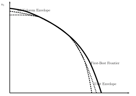
These theorems help us make some conjectures about the relative positions of the unit and ad valorem envelopes. One such conjecture is shown in Figure 1. The points where the two envelopes are tangent correspond either to some first-best situations (and hence with negative monopoly taxes) or to second-best situations where the monopoly tax is zero. There are situations where the unit envelope lies above the ad valorem envelope. These are associated with positive monopoly taxes. Then there are also situations where the reverse is true, and these are associated with negative monopoly taxes.
5. Concluding Remarks
In a general equilibrium model with a monopoly sector we have shown that the set of Pareto optima in a unit-tax economy neither dominates the set of ad valorem-tax Pareto optima nor is it dominated by it. If the shares in the private sector profits are equal for all consumers (which is equivalent to one hundred per cent profit taxation) the two sets of Pareto optima coincide. This conclusion is at odds with most of the existing literature relating unit taxation to ad valorem taxation.
6. Appendix A
This appendix contain the proofs of all of the theorems in the paper. The following ap-pendix rationalizes some of the assumptions in Theorems 1 and 2 in terms of the underlying primitives of the problem in so far as possible.
Proof of Theorem 1:
Our utility normalization and Assumptions (i), (ii), and (iv) of the theorem imply that
ρu(Au) is homeomorphic to ∆H−1, where the homeomorphism isκ:ρu(Au)→∆H−1 with
image
κ(u) = u
||u||, (6.1)
for every u = (u1, . . . , uH) ∈ ρu(Au).26 Note if u ∈ ρu(Au), then by our normalization u≥0H.27
Define the inverse of κ as K: ∆H−1 →ρu(Au).28
Define the correspondence T :Au×Sbu→∆H−1 as
T(z, π) = {β ∈∆H−1|βh = 0 if there exists h such that
q0xh0(z) +qTxh(z) +q0ω0h+qTωh> rah(z, π, θh)}.
(6.3)
We claim that T is non-empty, compact, convex valued, and upper-hemi continuous. It is trivial to prove thatT is nonempty and convex valued. We now show that it is upper-hemi continuous, which will imply that it is compact valued, given Assumptions (iii) and (iv). Suppose (zv, πvi → (z, πi ∈Au×Sbu and βv →β such that βv ∈ T(zv, πv) for all v. We need to show that β ∈ T(z, π). If there exists h such that q0xh0(z) +qTxh(z) + q0ω0h+ qTωh−ruh(z, π, θh)>0 then, by the definition of the mapping T, we have βh = 0. Since the functionsrah are continuous for allhinz andπ, there existsv0such that for allv ≥v0, we have qv0xh0(zv) +qvTxh(zv) +qv0ω0h+qvTωh−rah(zv, πv, θh)>0. Henceβhv = 0 for all
v ≥v0. Therefore βv →β implies that βh = 0.
The idea of correspondence T is to penalize (reduce utility of consumers) whenever the allocation and producer prices and tax combination (z, πi is such that the imputation of consumption bundles at consumer prices exceeds the income made available through profit shares and demogrant, evaluated at producer prices and taxes corresponding to π.
26 See also Quinzii, p. 51.
27 For H > 1, we can show that u6= 0H if u ∈ ρu(Au). For, suppose u = 0H. Then for any other
u0∈ρu(Au) (such au0exists otherwiseρu(Au) would be a singleton and hence zero dimensional manifold, contradicting assumption (iv)), there exists h such that u0h < uh (by definition of Pareto optimality), and hence u0h <0, which is a contradiction to our normalization of the utility functions (for under that normalization,u≥0 for allu∈ρu(Au)). Note also that, ifκ(ρu(zuh)) =α, thenαh= 0 andPh06=hαh0 = 1.
28 Its image is
K(α) =λ(α)α (6.2)
Define the correspondence K : ∆H−1×Sbu→∆H−1×Sbu, as
K(α, π) = (T(ρu−1(K(α)), π), Ψap(ρu−1(K(α)))). (6.4)
Under the maintained assumptions of this theorem, this correspondence is convex valued and upper-hemi continuous. The Kakutani’s fixed point theorem implies that there is a fixed point (α,∗ π∗i such thatα∗ ∈T(ρu−1(K(α∗)),π∗) and π∗ ∈Ψap(ρu−1(K(α∗))).
Let z∗ := ρu−1(K(α∗)). Hence, z∗ ∈ A and is unique (as ρu and K are bijective). From Assumption 6, we have
rhu ≤rah(z, ψpu(z), θh),∀h∈ H,and ∀z ∈Au. (6.5)
We now prove that
rah(z ,∗ π, θ∗ h) =q0(z∗)xh0(z∗) +qT(z∗)xh(z∗) +q0(z∗)ω0h+qT(z∗)ωh, ∀h∈ H. (6.6)
If there exists h such that
rah(z ,∗ π, θ∗ h)< q0(z∗)xh0(z∗) +qT(z∗)xh(z∗) +q0(z∗)ωh0 +qT(z∗)ωh, (6.7)
then by the definition of the correspondence T, we have α∗h = 0. By the definition of the homeomorphism K, this would imply u∗h = 0, and by our utility normalization, we will have (xh0(z∗), xh(z∗)) = (x0h(zuh), xh(zuh)), so that the right-hand side of (6.7) is rhu. This means that (6.7) contradicts (6.5). Hence, we have
rah(z ,∗ π, θ∗ h)≥q0(z∗)xh0(z∗) +qT(z∗)xh(z∗) +q0(z∗)ω0h+qT(z∗)ωh, ∀h∈ H, (6.8)
which implies
rah(z ,∗ π, θ∗ h)−
q0(z∗)xh0(z∗) +qT(z∗)xh(z∗) +q0(z∗)ω0h+qT(z∗)ωh
≥0, ∀h∈ H. (6.9)
Now monotonicity of preferences (in Assumption (i)) implies that at the Pareto optimal allocationz∗, we will have
X
h
xh(z∗) +ω=yc(z∗)−ym(z∗)−yg(z∗) +ω and
X
h
xh0(z∗) +ω0=y0(z∗) +ω0.
(6.10)
From second last equality in (3.20) and by multiplying the system in (6.10) by q(z∗) and q0(z∗) and adding, we have
X
h
rah(z ,∗ π, θ∗ h) =qT(z∗)[yc(z∗)−ym(z∗)−yg(z∗)] +q0(z∗)y0(z∗) +qT(z∗)ω+q0(z∗)ω0
=q0(z∗)
X
h
xh0(z∗h) +qT(z∗)X
h
xh(z∗) +qT(z∗)ω+q0(z∗)ω0.
This implies that
X
h
rah(z ,∗ π, θ∗ h)− qT(z∗)xh(z∗) +q0(z∗)xh0(z∗) +qT(z∗)ωh+q0(z∗)ωh0
= 0 (6.12)
Since (6.9) holds, (6.12) is true iff (6.9) holds as an equality, that is,
rah(z ,∗ π, θ∗ h) = qT(z∗)xh(z∗) +q0(z∗)xh0(z∗) +q0(z∗)ω0h+qT(z∗)ωh=wh(z∗), ∀h∈ H. (6.13)
From (6.13) we have for allh∈ H
ruh(z , ψ∗ up(z∗), θuh(z∗)) =wh(z∗) = rah(z , ψ∗ pa(z∗), θh) (6.14)
This proves (a).
The price and the ad valorem tax configuration ψpa(z∗) = (pa0(z∗), τ0(z∗), p(z∗), τ(z∗))
and the income configuration hrah(z , ψ∗ pa(z∗), θh)i define an ad valorem tax equilibrium of the private ownership economy hθhi, the underlying equilibrium allocation is z∗ and
the consumer prices are (q0(z∗), qT(z∗)) = (pa0(z∗)[1 +τ0(z∗)], pT(z∗)[IN +τττ(z∗)]) = (pu0(z∗) + t0u(z∗), p(z∗) +t(z∗)). This proves (b).
Denote MΠu(z∗) = Πmu(z∗) + Πc(z∗), MΠa(z∗) = Πma(∗z) + Πc(z∗), MGu(z∗) = t0(z∗)y0(z∗) + tT(z∗)[yc(z∗)−ym(z∗)−yg(z∗)]−pT(z∗)yg(z∗),and MGa(z∗) =pa0(z∗)τ0(z∗)y0(z∗)+pT(z∗)τττ(z∗)[yc(z∗)− ym(z∗)−yg(z∗)]−pT(z∗)yg(z∗). At z∗ we know, from (3.20), that the sums of profits and government revenue are the same under the unit and ad valorem systems, that is
MΠu(z∗) +MGu(z∗) =MΠa(z∗) +MGa(z∗)
⇔ −[MΠa(z∗)−MΠu(z∗)] = MGa(z∗)−MGu(z∗). (6.15)
From conclusion (a) we have for all h∈ H
wh(z∗) = θuh(z∗)MΠu(z∗) + 1
HM u
G(z∗) =θhMΠa(z∗) +
1
HM a G(z∗)
⇒θhu(z∗)MΠu(z∗)−θhMΠa(z∗) =
1
H[M a
G(z∗)−MGu(z∗)]
⇒θhu(z∗)MΠu(z∗)−θhMΠa(z∗) =
1
H[M u
Π(z∗)−MΠa(z∗)].
(6.16)
The last equality follows from (6.15). Hence, (6.16) implies that θhu(z∗) =θh for all h∈ H
iff θh = H1 for allh ∈ Hor MΠu(z∗)−MΠa(z∗) = 0. The latter is true when t0(z∗) = 0. Thus,
(c) is true.
We now prove (d). Let u∗:=ρu(z∗).
If u∗ ∈ Uu(hθhi) := {huhi ∈ RH|u1 ≤ Uu(u2, . . . , uH,hθhi)}, then since u∗ ∈ ρu(A), we
have, because of Assumption (vi), the unique solution to (3.2) as
∗
From (c) this is true iff θh= H1 for all h∈ H or t0(z∗) = 0.
If θh = H1 for all h ∈ H or t0(z∗) = 0, then again (6.17) follows from (c), and we have
∗
u∈Uu(hθhi) :={huhi ∈ H|u1 ≤ Uu(u2, . . . , uH,hθhi)}.
Proof of Theorem 2: We write the Lagrangian of problem (4.2) as
L=−X
h
¯
sh[uh−Vh()]−¯vT[x()−yc() +ym() +yg]−v¯0[x0()−y0u]−β¯[pu0 −P0u()]
−X
h
¯
αh
wh−θh[pu0y0u−C() + Πc()]−
1
H [t T
(yc−ym−yg) +t0y0−pyg ]
−r¯[g−F(yg)]−γ¯[X
h
θh−1]−X
h
¯
φh[θh−1],
(6.18) where ¯s1 = 1. Assuming interior solutions for variablespu0, p, t0, t,andhwhi, the first-order
conditions include
−X
h
¯
shxh0 −¯vT∇q0x−v0¯ ∇q0x0+ X
h
¯
αhy0uθh−β¯= 0, (6.19)
−X
h
¯
shxh0 −¯vT∇q0x−v0¯ ∇q0x0+ X
h
¯
αhy0u
1
H + ¯β∇t0P
u
0 = 0, (6.20)
−X
h
¯
shxhT −¯vT∇qx+ ¯vT[∇pyc− ∇pym]−v¯0∇Tqx0
+X
h
¯
αh
θh[−∇TpC+∇TpΠc] +
1
H[t T(∇
pyc− ∇pym)−ygT]
+ ¯β∇TpP0u= 0,
(6.21)
−X
h
¯
shxhT −v¯T∇qx−v0¯ ∇Tqx0+ X
h
¯
αh
1
H[y cT −
ymT −ygT] + ¯β∇TtP0u = 0, (6.22)
¯
sh−¯vT∇whx h−¯v
0∇whx h
0 −α¯h+ ¯β∇whP u
0 = 0, for h∈ H, (6.23)
¯
vT = ¯r∇TygF − X
h
¯
αh 1 H[t
T +pT], (6.24)
and
¯
vT∇yu 0y
m = ¯v 0+ X h ¯ αh
θh[pu0 − ∇yu 0C] +
1
H[−t T∇
yu 0y
m+t 0 ]
. (6.25)
We also have the following Kuhn-Tucker conditions for hθhi and the Lagrange multipliers
hφ¯hi
¯
αh[pu0y0u−C() + Πc()]−¯γ+ ¯φh≤0, θh ≥0 and θh[ ¯αh[pu0yu0 −C() + Πc()]−¯γ+ ¯φh] = 0, ∀h∈ H,
and
θh−1≤0, φ¯h ≥0, and ¯φh[θh−1] = 0, ∀h∈ H. (6.27)
The system can be simplified further. Subtract (6.20) from (6.19) to get
¯
β[1 +∇t0P
u 0] =y0u
X
h
¯
αh[θh−
1
H]. (6.28)
Subtract (6.22) from (6.21) to get
[¯vT+X
h
¯
αh Ht
T
][∇pyc−∇pym]+[ycT−ymT] X
h
¯
αh[θh−
1
H]+ ¯β[∇ T
pP0u−∇TtP0u] = 0. (6.29)
Let hθhi = hθ∗uh(u2, . . . , uH)i. Then θh > 0 for all h ∈ H. Hence, from (6.27), we have φh = 0 for all h, and (6.26) implies that
¯
αh[pu0y0u−C() + Πc()] = ¯γ, ∀h∈ H. (6.30)
which correspond to variables (θh)h. Now, (6.30) implies
¯
αh=
¯
γ
pu0y0u−C() + Πc() =:K, ∀h (6.31)
Given that P
hθh= 1, (6.31) implies that at any optimum,
X
h
¯
αh[θh− 1
H] =K
X
h
[θh− 1
H] = 0. (6.32)
Thus, (6.32) and (6.28), and the assumption that ∇t0P
u
0 6=−1 imply that
¯
β = 0, (6.33)
i.e.,the monopoly constraint is non-binding at the solution to problem (4.2). From (6.29), (6.32), and (6.33), we have
[¯vT +X
h
¯
αh Ht
T][∇
pyc− ∇pym] = 0. (6.34)
Homogeneity of degree zero in p of the competitive supplies and the monopolist’s cost minimizing input demands implies
[¯vT +X
h
¯
αh Ht
T] =µpT, (6.35)
which from (6.24), implies
¯
r∇TygF = (µ+K)pT. (6.36)
Now, (i) using (6.33) and (6.31), (ii) post multiplying (6.22) by xh0, summing up over all
h, and subtracting from (6.22), and (iv) recalling that at a tight equilibrium, we have
P
hxh=yc−ym−yg and y0u =
P
hxh0, we obtain
¯
vT v0¯ X
h
∇q0x
h+∇ whx
hxh
0 ∇qxh+∇whx hxhT
∇q0x
h
0+∇whx h
0xh0 ∇qxh0+∇whx h 0xhT
=
0T 0. (6.37)
But the second matrix on the left-handside of (6.37) is the sum over all h ∈ H of Slut-sky matrices of price derivatives of compensated demands of the consumers. Since, by assumption, each of these matrices has rank N, we have
¯
vT v0¯ =κ
qT q0 =κ
pT +tT pu0+t0. (6.38)
Employing (6.31), (6.35), and (6.38), we have
κ[pT +tT] +KtT =µpT
⇒κ[pT +tT] +K[tT +pT] = [µ+K]pT
⇒ κ+K
µ+Kq
T =pT
(6.39)
From (6.31), (6.38), and (6.25), and exploiting the homogeneity properties of the cost function, we have
µ∇yu
0C =κq0+K[q0− ∇y0uC]
⇒ κ+K
µ+Kq0=∇yu0C
(6.40)
By choosing ¯r, κ, µ, and K such that µκ++KK = 1 and ¯r = κ+K, we obtain from (6.36),
(6.39), and (6.40)
∇TygF =qT =pT and
∇yu
0C =q0.
(6.41)
Thus (6.41) is reflective of joint consumption and production efficiency at the solution of program (4.2). Hence, the allocation corresponding to a solution of program (4.2) is a first best Pareto optimal allocation.
Proof of Theorem 3:
(ii) Suppose ∃h0 such that θh0 = 0. The unit shares that make z a unit tax equilibrium
(lying on the unit envelope) are given by
θuh(z) = θhM
a
Π(z) + H1[M a
G(z)−MGu(z)]
MΠu(z) ≥0, ∀h∈ H. (6.42)
So for h0, we have
θuh0(z) =
1
H[MGa(z)−MGu(z)]
From (4.3) this implies that t0(z) ≥ 0. We prove that t0(z) = 0. Suppose not. Then t0(z)>0. This means, from (4.3), that
θuh(z) = θhM
a Π(z) +
1
H[MGa(z)−MGu(z)]
MΠu(z) >0,∀h∈ H. (6.44)
Thus z is on the unit envelope with θhu(z) >0 for all h∈ H. This implies from Theorem 2 that z is first-best. But this contradicts Remark 2 based on GL, which says t0(z) < 0
for a first-best allocation with a unit-tax representation. Hence t0(z) = 0. This means MΠa(z) =MΠu(z). Combined with (4.3) and (6.42) we get θh =θuh(z) for all h∈ H.
(i) Suppose θh >0 for all h∈ H. Two case are possible from viewing (6.42).
(a) θuh(z)>0 for allh∈ H. Thus z is on the unit envelope with θuh(z)>0 for all h∈ H. This implies from Theorem 2 that z is first-best. Remark 2 based on GL, implies
t0(z)<0.
(b) There exists h0 such that θuh0(z) = 0. (6.42) implies that
0 = θh0MΠa(z) + 1
H[M a
G(z)−MGu(z)]. (6.45)
Since θh >0 for all h ∈ H, including h0 by assumption and profits are not zero, this implies
θh0MΠa(z) =
1
H[M u
G(z)−MGa(z)]>0. (6.46)
From (4.3), this means t0(z) < 0. So either z is a first-best (with constraints in
Theorem 2 just binding) or is an ad valorem equilibrium with positive shares on the unit envelope. The analogue of Theorem 1 for the ad valorem-tax envelope implies that z does not lie on the ad valorem envelope (as any ad valorem equilibrium on the ad valorem envelope with positive shares is a first-best by the analogue of Theorem 2, which gives the relation between the first-best frontier and the ad valorem-tax envelope). Hence the ad valorem envelope lies above the unit envelope for the utility profile ρu(z).
Proof of Theorem 4:
(i) Suppose θh > 0 for all h∈ H. The ad valorem shares that make z an ad valorem tax equilibrium (lying on the ad valorem envelope) are given by
θah(z) = θhM
u Π(z) +
1
H[MGu(z)−MGa(z)]
MΠa(z) ≥0, ∀h∈ H. (6.47)
Two cases are possible from (6.47):
(a) θah(z) > 0 for all h ∈ H. Since we are on an ad valorem envelope, the analogue of Theorem 2 for ad valorem-tax envelope implies that z is a first-best.
(b) There exists h0 such that θah0(z) = 0. (6.47) implies that
θah0(z) = 0 =θh0MΠu(z) + 1
H[M u
Which implies, because θh>0 for all h∈ H in case (i) of this theorem, that
θh0MΠu(z) =
1
H[M a
G(z)−MGu(z)]>0. (6.49)
From (4.3), this means that τ0(z) > 0 or t0(z) > 0. So from Remark 2, we cannot
be on a first-best, at this point on the ad valorem envelope. Since this is a unit-tax equilibrium with positive shares, which is not on the first-best, from Theorem 2, we cannot be on the unit envelope. Hence the unit envelope lies above the ad valorem envelope at this utility profile ρa(z).
(ii) Suppose ∃h0 such thatθh0 = 0. Then from (6.47)
θha0(z) =
1 H[M
u
G(z)−MGa(z)]
MΠa(z) ≥0, ∀h ∈ H. (6.50)
From (4.3), this means that τ0(z)≤0 or t0(z)≤0. Two case are possible:
(a) τ0(z)<0. From (4.3), this would mean MGu(z)−MGa(z)>0, and hence from (6.50), this would mean θha(z)> 0 for all h ∈ H. Since we are on the ad valorem envelope, from the analogue of Theorem 2 for the ad valorem envelope, this would mean that
z is first-best.
(b) τ0(z) = 0. This means MΠa(z) = MΠu(z). Combined with (4.3) and (6.50) we get θh=θha(z) for allh ∈ H.
7. Appendix B
The discussion and proofs in this appendix are for economies with unit taxes. Similar discussions and results can be obtained for the ad valorem tax case.
A tight unit-tax equilibrium is obtained by replacing the inequalities in (2.6) to (2.10) by equalities. We focus only on tight unit-tax equilibria. The domain of the vector of variables (pu0, p, t0, t,hwhi, y0, yg) is taken to be RN+++1 ×RN+1×RH++N+1, which we
denote by ΩE.
Note that the equilibrium system (2.6) to (2.10) is homogeneous of degree zero in the variables pu0, p, t0, t, and hwhi.29 So we can adopt a normalization rule to uniquely
determine prices, taxes, and incomes corresponding to equilibrium allocations.
A function b :R+×R×R+N ×RN ×RH+ →Rdefines a price-normalization rule b(p0, t0, p, t,hwhi) = 0 (7.1)
if it is continuous and increasing and there exists a function Bb:R+×R×RN+ ×RN →
R++, with image Bb(πp0, πt0, πp, πt), such that for every (πp0, πt0, πp, πt,hπwhii ∈ R+×
R×RN+ ×RN ×RH+,
b( πp0
Bb() , πt0
Bb() , πp
Bb() , πt
Bb() ,hπwh
Bb()
i) = 0 (7.2)
29 Recall, that the functionPu
Monotonicity of the function b implies that the function Bb is unique for a given function b.30 Let us choose an increasing and differentiable function b : ΩN → R, which
defines a valid price normalization rule in the sense of that defined in the earlier section31
b(p0, t0, p, t,hwhi) = 0. (7.3)
Under such a normalization rule and some regularity assumptions, the set of all (tight) unit tax equilibria can be shown to be generically a 2N−1 dimensional manifold. Lemma A1 below demonstrates this. Define the function: F : ΩE →RN+H+4 with image
F(p0, p, t, t0,hwhi, y0, yg) as
−x(p0+t0, p+t,hwhi) +yc(p)−ym(y0u, p)−yg
−x0(p0+t0, p+t,hwhi) +yu0 pu0 −P0u(p, t0, t,hwhi)
wh−
θh[pu0y0u−C(yu0, p) + Πc(p)] +
1
H[t
T(yc(p)−ym(yu
0, p)−yg) +t0y0u−pyg]
, ∀h
F(yg)−g
b(p0, t0, p, t,hwhi).
(7.4)
Lemma A1: Suppose F is a differentiable mapping and there exists a neighborhood
E around 0 in RN+H+4 such that for all ν ∈ E, F−1(ν) 6= ∅. Then for almost all
ν ∈ E (that is, except for a set of measure zero in E), F−1(ν) is a manifold of dimension 2N −1 = 3(N + 1) +H−[N +H+ 4].
The proof follows from Sard’s theorem.32 This lemma implies that the set of regular economies which differ from the original one only in terms of endowments is very large (this set is dense).
Suppose F is differentiable. Denote the derivative of F, evaluated at v ∈ΩE as the
linear mapping ∂Fv : ΩE →RN+H+4 where ∂Fv is the Jacobian matrix, evaluated at v
∂Fv =
JE1 JE2 JE3 JE4 JE5
, (7.5)
30 Some examples:
(i) b(p0, t0, p, t,hwhi) =k hp0, t0, p, ti k −1 andBb(p0, t0, p, t) =k hp0, t0, p, ti k
(ii) b(p0, t0, p, t,hwhi) =p1−1 andBb(p0, t0, p, t) =p1
(iii) b(p0, t0, p, t,hwhi) =p0+P N
k=1pk−1 andBb(p0, t0, p, t) =p0+P N k=1pk. 31 ΩN :=RN+++1×RN+1×RH+.
with
JE1= [JE11 JE21]
JE11=
−∇
q0x −∇q0x −∇qx −∇qx− ∇
T
pym+∇pyc −∇w1x
1 . . . −∇ wHx
H
−∇q0x0 −∇q0x0 −∇qx0 −∇qx −∇w1x
1
0 . . . −∇wHx H 0
JE21=
−∇
y0y
m −I
1 0TN
.
(7.6)
JE2 = [JE12 JE22]
JE12 =
−H1y0 −θ1y0u −H1[ycT −ymT −yg] −θ1[ycT −ymT] +H1ygT 1 0 . . . 0
.. .
−H1y0 −θHy0u −H1[ycT −ymT −yg] −θH[ycT −ymT] + 1
HygT 0 0 . . . 1
JE22 =
θ1∇y0C−
1 Ht0
1 HPT
.. .
θH∇y0C−
1 Ht0
1 HP T . (7.7)
JE3=
−∇t0P
u
0 1 −∇Tt P0u −∇TpP0u −∇h1P
u
0 . . . −∇wHP u
0 0 0TN
, (7.8)
JE4=
0 0 0TN 0TN 0 . . . 0 0 ∇T
ygF, (7.9)
and
JE5 =
∇t0b ∇p0b ∇
T
tb ∇Tpb ∇w1b . . . ∇wHb 0 0 T N
. (7.10)
By stacking the matrices above and looking at the structure of ∂Fv, it can be seen that ∂Fv, which is of dimension (N+H+ 4)×3(N + 1) +H, has at least rank N +H+ 2 for
allv ∈ΩE. There are at least N +H+ 2 columns in ∂Fv which are linearly independent
for all v ∈ΩE. These are columns that correspond to the variables yg, y0, hwhi, and p0.
Lemma A2: Suppose F is a differentiable mapping, F−1(0) 6= ∅, and 0 is a regular
value of F (that is, the rank of ∂Fv is N +H+ 4 for all v ∈ F−1(0)). Then F−1(0) (the
set of all tight tax equilibria) is a manifold of dimension 2N −1.
The proof follows from the pre-image theorem.
Assumption A1: The set of tight tax equilibria F−1(0) is a subset of the interior of ΩE
Consider problem that identifies the Pareto manifold for a hθhi ∈ ∆H−1 economy. Using (3.1) and our normalization rule, the programme can be rewritten as
Uu(u2, . . . , uH,hθhi) := max pu0,p,t0,t,hwhi,y0,yg
V1(pu0+t0, p+t, w1)
subject to
Vh(pu0 +t0, p+t, wh)≥uh, ∀h= 2, . . . , H,
−x(pu0 +t0, p+t,hwhi) +yc(p)−ym(p, y0u)−yg≥0
−x0(pu0 +t0, p+t,hwhi) +y0u≥0 pu0−P0u(p, t0, t,hwhi) = 0,
wh=θh[pu0yu0 −C(y0u, p) + Πc(p)] +
1
H [t
T(yc−ym−yg) +t
0y0−pyg ], ∀h, F(yg)−g ≥0,
b(pu0, t0, p, t,hwhi) = 0.
(7.11) We write the Lagrangian as
L=−X
h
¯
sh[uh−Vh()]−¯vT[x()−yc() +ym() +yg]−v¯0[x0()−y0u]−β¯[pu0 −P0u()]
−X
h
¯
αh
wh−θh[pu0y0u−C() + Πc()]−
1
H [t
T(yc−ym−yg) +t
0y0−pyg ]
−r¯[g−F(yg)]−δ b¯ (p0, t0, p, t,hwhi),
(7.12) with ¯s1 = 1, ¯sh ≥0 for all h= 2, . . . , H, ¯v ≥0N, ¯v0 ≥0, ¯r≥0, and the signs of the other
Lagrange multipliers (those corresponding to equality constraints) being unrestricted.33 Suppose Assumption A1 holds and all solutions to (7.11) involve tight tax equilibria. The first order necessary conditions of this problem, for any utility profile (u2, . . . , uH) for
which solution exists, include
(a) those (3(N + 1) +H of them) obtained by taking the derivatives of the Lagrangian with respect to the choice variables,
−X
h
¯
shxh0 −v¯T∇q0x−v¯0∇q0x0+ X
h
¯
αhyu0θh−β¯−¯δ∇p0b = 0, (7.13)
−X
h
¯
shxh0 −v¯T∇q0x−¯v0∇q0x0+ X
h
¯
αhy0u
1
H + ¯β∇t0P
u
0 −δ¯∇t0b = 0, (7.14)
33 Note, in general, the signs of the Lagrange multipliers are specific to the way in which one sets up the optimization. If we were optimizing consumerh’s utility keeping utility of consumers 1, . . . , h−1, h+ 1, . . . , H fixed then the sign restrictions on the vector ¯swould be different (¯sh= 1 and ¯sh0 ≥0, ∀h06=h.