University of Warwick institutional repository: http://go.warwick.ac.uk/wrap
This paper is made available online in accordance with
publisher policies. Please scroll down to view the document
itself. Please refer to the repository record for this item and our
policy information available from the repository home page for
further information.
To see the final version of this paper please visit the publisher’s website.
Access to the published version may require a subscription.
Author(s): M. Kuster, J. Wilms, R. Staubert, W. A. Heindl, R. E.
Rothschild, K. A. Postnov, N. I. Shakura
Article Title: Probing the outer edge of an accretion disk: a Her X-1
turn-on observed with RXTE
Year of publication: 2005
Link to published article:
http://dx.doi.org/10.1051/0004-6361:20042355
Publisher statement: © ESO 2005. M. Kuster et al. (2005). Probing the
outer edge of an accretion disk: a Her X-1 turn-on observed with
DOI: 10.1051/0004-6361:20042355 c
ESO 2005
Astrophysics
&
Probing the outer edge of an accretion disk: a Her X-1 turn-on
observed with
RXTE
M. Kuster
1,2, J. Wilms
3, R. Staubert
4, W. A. Heindl
5, R. E. Rothschild
6, N. I. Shakura
7, and K. A. Postnov
7,81 Technische Universität Darmstadt, Institut für Kernphysik, Schlossgartenstr. 9, 64289 Darmstadt, Germany
e-mail:[email protected]
2 Max-Planck-Institut für extraterrestische Physik, Giessenbachstr., 85748 Garching, Germany
3 Department of Physics, University of Warwick, Coventry, CV7 4AL, UK 4 Institut für Astronomie und Astrophysik, Sand 1, 72076 Tübingen, Germany
5 SAIC, 16701 West Bernardo Drive, San Diego, CA 92127, USA
6 Center for Astrophysics and Space Sciences, UCSD, La Jolla, CA 92093, USA
7 Sternberg Astronomical Institute, Moscow State University, 119899 Moscow, Russia 8 Faculty of Physics, Moscow State University, 119899 Moscow, Russia
Received 10 November 2004/Accepted 29 June 2005
ABSTRACT
We present the analysis of Rossi X-ray Timing Explorer (RXTE) observations of the turn-on phase of a 35 day cycle of the X-ray binary Her X-1. During the early phases of the turn-on, the energy spectrum is composed of X-rays scattered into the line of sight plus heavily absorbed X-rays. The energy spectra in the 3–17 keV range can be described by a partial covering model, where one of the components is influenced by photoelectric absorption and Thomson scattering in cold material plus an iron emission line at 6.5 keV. In this paper we show the evolution of spectral parameters as well as the evolution of the pulse profile during the turn-on. We describe this evolution using Monte Carlo simulations which self-consistently describe the evolution of the X-ray pulse profile and of the energy spectrum.
Key words.stars: individual: Hercules X-1 – X-rays: binaries – stars: neutron – accretion, accretion disks – scattering
1. Introduction
Her X-1 is one of the best understood X-ray binary sys-tems showing a variety of long and short term periodicities. The X-ray pulsar spins with a 1.24 s period and moves in a 1.7 day almost circular orbit around its companion HZ Her (Tananbaum et al. 1972). Both effects cause a modulation of the observed flux in optical as well as in the X-rays. In addition the X-ray light curve of Her X-1 shows a long term 35 day intensity variation. This modulation is the best evidence for an inclined, precessing, and warped accretion disk in an X-ray binary sys-tem. The origin of the warping is not yet fully understood, but may be caused either by radiation driven accretion disk winds (Schandl & Meyer 1994) or by radiation pressure (Maloney & Begelman 1997). The precessing motion of the disk can be understood in the context of tidal interaction and/or as a conse-quence of non vanishing torques acting on the disk, e.g. due to a coronal wind (Schandl & Meyer 1994; Schandl et al. 1997; Shakura et al. 1998; Ketsaris et al. 2001). Because of the high inclination of the system, the disk periodically blocks the line of sight to the neutron star during about 60% of the 35 day cycle.
The observed 35 day light curve shows two maxima in intensity: the “main-on” and the “short-on” (Giacconi et al. 1973). Following the often adopted baseline model of Her X-1
(Katz 1973; Schandl & Meyer 1994; Scott et al. 2000; Ketsaris et al. 2001; Leahy 2004,and references therein), the ∼12 day long main-on starts when the outer rim of the accretion disk opens the line of sight to the central neutron star (see Fig. 2). Subsequently, at the end of the main-on the inner edge of the accretion disk covers the line of sight. The second maximum in intensity occurs as soon as the inner edge of the accretion disk uncovers the line of sight during the progression of the 35 day cycle. This phase is called short-on where only∼35% of the main-on intensity is measured. The states in between the short-on and the main-short-on are called “low-states” where the intensity drops to∼3% of the main-on intensity (Scott & Leahy 1999). The transitions from the low-states to the main-on and short-on are called “turn-on”, while the decline in intensity at the end of the main-on and the short-on generally is called “turn-off”. This periodic behavior is irregularly interrupted by anomalous low states as it was observed in 1983 (Parmar et al. 1985), 1993 (Vrtilek et al. 1994; Vrtilek & Cheng 1996), 1999 (Parmar et al. 1999; Coburn et al. 2000; Oosterbroek et al. 2001), and recently in 2004 (Boyd et al. 2004). During an anomalous low state the maximum X-ray flux typically drops to 1–3% of the main-on flux.
While the end of the main-on has been the subject of previ-ous Ginga observations (e.g., Deeter et al. 1998), observational data on the spectral evolution during the start of the main-on
500 1000 1500 2000
2−40 keV
PCA Count Rate [cts/s]
00 0102 03
04 05
06 07
08 09
10 111213
14 15
16 1718
19 20
21 22
23 2425 26
2728 29
30
31
Eclipse
Pre−Eclipse Dip
Anomalous Dip
0 2 4 6 8
ASM
2−12 keV
Time [MJD]
[image:3.595.114.514.71.377.2]50704.0 50704.5 50705.0 50705.5 50706.0 50706.5 50707.0
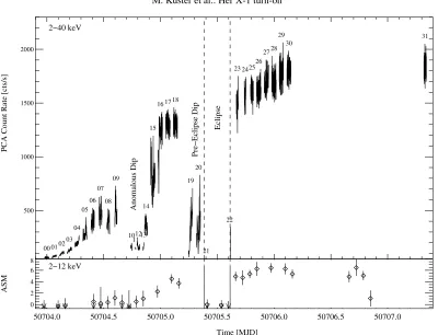
Fig. 1. From top to bottom: RXTE PCA and RXTE ASM count rates for the time of the turn-on. The beginning and the end of an eclipse are marked by dashed lines. The numbers identify individual RXTE orbits starting with orbit 00 to orbit 31.
has been rare. Observations of turn-ons of Her X-1 have been presented by Becker et al. (1977), Davison & Fabian (1977), and Parmar et al. (1980) with different instruments. All of these observations show a strong indication that the flux during the early stages of the turn-on is composed of heavily absorbed plus scatted radiation. In 1997 September we observed a com-plete turn-on of the 35 day cycle of Her X-1 in a two day continuous observation with the Rossi X-ray Timing Explorer (RXTE). In this paper we present results from the spectral and temporal analysis of this observation. Further we describe these data with a physical model that can reproduce the spectral fea-tures and temporal evolution of the pulse shape seen in this observation. For our physical model we assume that the varia-tions of the observed spectrum are due to the varying column density caused by cool gas of the outer rim of the accretion disk and due to radiation scattered from (ionized) gas sandwiching the accretion disk (an accretion disk corona).
The remainder of this paper is structured as follows: in Sect. 2 we give a short description of our observation and the extraction of the data, before we describe our spectral model and the results of the spectral analysis in Sect. 3, we present the results of our analysis of the evolution of the pulse profile in Sect. 4. In Sect. 5 we introduce a method to determine the amount of absorbed and scattered radiation by simulating the influence of a scattering medium on the shape of the pulse pro-file using Monte Carlo simulations. We summarize this paper in Sect. 6 and propose a model of the outer accretion disk rim which can explain the spectral behavior as well as the evolution of the pulse profile.
2. Observation and data reduction
We observed Her X-1 for two days on 1997 September 13/14 with RXTE. Figure 1 shows the RXTE Proportional Counter Array (PCA) light curve of the entire observation, together with the light curve measured simultaneously by the RXTE All Sky Monitor (ASM). Note that during the entire observation all five PCUs of the RXTE PCA were active and therefore throughout this paper the count rates are consistently given in cts/s for five PCUs. During the turn-on an eclipse took place around MJD 50705.5. Furthermore, two dips were detected: a pre-eclipse dip around MJD 50705.3 and an anomalous dip around MJD 50704.8. The gaps in the light curve are due to Earth oc-cultations and SAA passages during individual RXTE orbits. The exposure times, mean count rates, and dates of observa-tion are given in Table 1 for each RXTE orbit.
For the detailed analysis, we extracted PCA light curves for all RXTE orbits listed in Table 1 with a time resolu-tion of 16 ms. Light curves were extracted for five energy bands: 2.0–4.5 keV, 4.5–6.5 keV, 6.5–9 keV, 9–13 keV, and 13–19 keV. After correcting the photon arrival times with re-spect to the solar systems barycenter and for the orbital mo-tion of the neutron star, we determined the pulse period of Her X-1 by folding the data of the 13–19 keV energy band using a χ2 maximization test. The resulting pulse period is PSpin =1.2377291(2) s (MJD 50708.199), which is consistent with observations of, e.g., Dal Fiume et al. (1998) and Coburn et al. (2000). Subsequently we folded all light curves with this pulse period to obtain a pulse profile for each energy band and
Table 1. Observing log of the turn-on observations of Her X-1.
Obs. Date Exposure Count rate
[MJD] [s] [counts s−1] 00 50703.979 3300 62.1±0.2 01 50703.979 3400 73.3±0.3 02 50703.979 3300 100.0±0.3 03 50703.979 3300 130.0±0.3 04 50703.979 3200 195.4±0.3 05 50704.312 3000 280.8±0.4 06 50704.312 2600 402.7±0.5 07 50704.452 2300 469.2±0.5 08 50704.452 2100 395.0±0.5 09 50704.452 1700 501.7±0.6 10 50704.727 1200 158.8±0.5 11 50704.727 300 148.7±1.0 12 50704.727 2100 160.6±0.4 13 50704.727 700 156.7±0.7 14 50704.860 2100 358.4±0.5 15 50704.860 3400 813.6±0.5 16 50704.860 3300 1197.0±0.6 17 50705.045 3400 1298.1±0.7 18 50705.045 3200 1293.7±0.7 19 50705.045 3100 325.6±0.4 20 50705.312 3000 329.3±0.4 21 50705.381 2700 34.9±0.3 22 50705.591 1800 73.2±0.4 23 50705.659 1500 1494.1±1.1 24 50705.726 1200 1568.2±1.2 25 50705.793 2100 1607.3±0.9 26 50705.793 3300 1612.5±0.7 27 50705.793 3400 1697.5±0.7 28 50705.793 3400 1699.1±0.7 29 50705.793 3100 1787.7±0.8 30 50706.096 3100 1810.4±0.8 31 50707.313 1900 1828.2±1.0
Exposure times shown are rounded to the closest 100 s. The count rate is background subtracted.
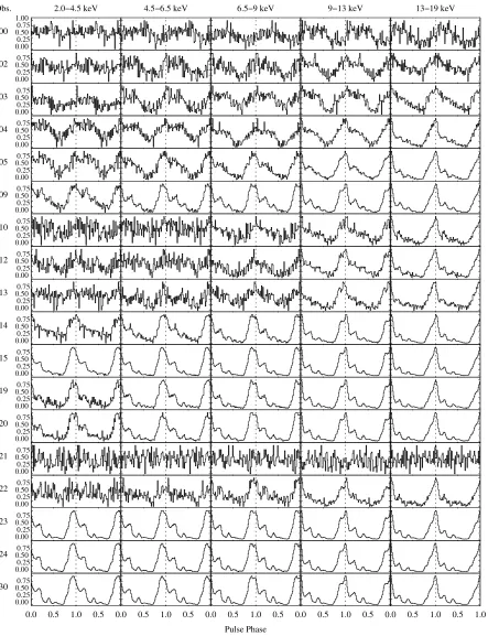
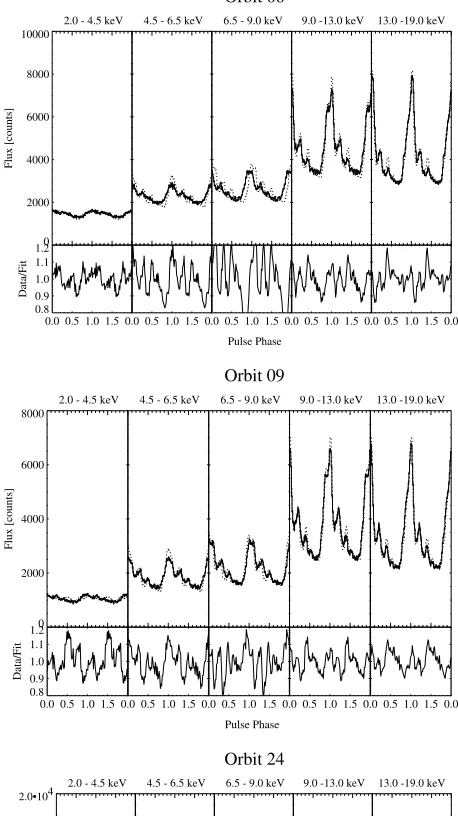
[image:4.595.334.492.120.178.2]the maximum flux in the main pulse of the profile in the en-ergy range 13–19 keV. From each profile we subtracted the unpulsed flux and normalized the count rate to the maximum. Figure 6 shows the evolution of the pulse profiles in different energy ranges over the time of the whole turn-on. We have omitted those orbits during which the pulse profile shows no remarkable variation compared to the previous or following or-bit, i.e., the orbits 01, 06–08, 16–18, and 25–30.
For the spectral analysis, pulse phase averaged PCA and
HEXTE spectra were extracted for each individual RXTE orbit.
To minimize the background, we have chosen good-time inter-vals (GTI) with an “electron-ratio” of all PCUs less than 0.1 (see e.g., Wilms et al. 1999). All spectra are background and dead-time corrected. The data of orbits 10–14 and 19–22 were omitted for the analysis because our spectral model is not
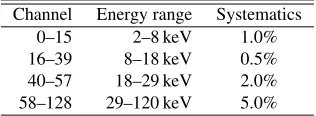
Table 2. Systematic errors applied to the PCA data to account for un-certainties in the PCA response matrix.
Channel Energy range Systematics
0–15 2–8 keV 1.0%
16–39 8–18 keV 0.5%
40–57 18–29 keV 2.0%
58–128 29–120 keV 5.0%
applicable during the times of the dips and the eclipse. We si-multaneously fitted our spectral model described in Sect. 3.1 to both the HEXTE and PCA data of each orbit. The systematic uncertainties of the response matrix of the PCA assumed for the spectral analysis are given in Table 2.
3. Evolution of spectral parameters
Before we present the results of our spectral fitting in Sect. 3.2, we give an introduction to the complex spectral model used to describe the data.
3.1. Spectral model
As earlier observations already have shown (Davison & Fabian 1977; Parmar et al. 1980; Becker et al. 1977), a combination of direct, scattered, and absorbed photons is observed during the turn-on. Therefore, we used a partial covering model which combines both, scattering and absorption, to fit the data over the time of the turn-on. As components for the spectral model we used an exponentially cutoffpower-law Ipower(E)·Ihighecut(E) as implemented in XSPEC, a cyclotron line feature Icyc(E) at 39 keV using thecyclabs model of XSPEC, and a Gaussian emission line IFe(E) fixed at 6.4 keV. For an analytic descrip-tion of the individual model components we refer the reader to
theXSPECmanual (Arnaud & Dorman 2002).
We combined these four spectral components to provide a basic continuum model, which is then observed through an ab-sorber partially covering the continuum source. In an analytic form the final spectral model describing the photon spectrum can then be written as
I(E)=B·(1+a(E))· (I0(E)+IFe(E)) Primary Spectrum
(1)
with
a(E)= e−NHσT Thomson-Scattering
·C · e−NHσbf
Absorption
(2)
and
Neutron Star
Accretion Disk Corona
Accretion Disk
Observer
D C A
[image:5.595.64.300.77.215.2]B
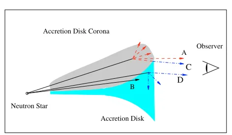
Fig. 2. Schematic illustration of the geometry during a turn-on of Her X-1 (not to scale). The accretion disk rim, the accretion disk corona, and the neutron star are shown. Three different components contributing to the overall observed flux are indicated: radiation ab-sorbed by the cold material of the accretion disk (photons following beam A), radiation absorbed by the accretion disk rim and further re-duced in flux by Thomson scattering (photons following beam B), and radiation scattered by the corona into the line of sight of the observer (photons following beam C).
the relative ratio of absorbed and scattered radiation to the un-affected radiation. A larger value of C implies a larger degree of absorbed and scattered flux. From now on, in the rest of this article the unaffected model component will be called MC I and the component influenced by absorption and Thomson scat-tering will be referenced as MC II. For the model compo-nent MC I we neglected Galactic absorption since the Galactic
NH=1.79×1020cm−2 is small compared to the NHof model component MC II. A schematic picture illustrating the geomet-ric situation during the turn-on is shown in Fig. 2. The positions of the accretion disk and an accretion disk corona relative to the neutron star are shown. Photons following beam A, marked by a dashed line, are scattered in the corona and can be partially absorbed in the accretion disk rim (beam C, dash dotted line). While a certain fraction of photons are blocked by the accretion disk (beam B), the outer parts of the accretion disk are optically thin for X-rays. Therefore, the spectral distribution of photons following beam D will show strong signature of photoelectric absorption. To simplify matters, photons reaching the observer directly without being modified by either the accretion disk nor the accretion disk corona are not shown in Fig. 2. Comparing this geometric interpretation with the spectral model given in Eq. (2) allows the following interpretation:
– The unaffected model component I(E) = I0(E)+IFe(E), called MC I from now on, accounts for photons following beam A and photons reaching the observer directly (this case is not shown in Fig. 2).
– The model component modified by photoelectric
absorp-tion and Thomson scattering I(E)=a(E)·(I0(E)+IFe(E)), called MC II from now on, represents the spectral distribu-tion of photons following beam C and beam D.
We emphasize that it is not possible to use a physically more realistic spectral model which treats scattered, absorbed, and direct flux separately. The problem lies within the nature of Thomson scattering: for photon energies E 10 keV (E
mec2) and when the influence of multiple scatterings can be
Table 3. Parameters fixed to their mean value for the fitting of the spectra over the time of the turn-on.
Parameter Value
α 1.068
Ecutoff 21.5 keV
Efold 14.1 keV
Ecyc 39.4 keV
σcyc 5.1 keV
EFe 6.45 keV
σFe 0.45 keV
neglected (τ5), scattering of photons by stationary and free electrons can be treated as elastic and consequently energy in-dependent (classical Thomson approximation). This makes it impossible to separate, e.g., the direct flux and the flux contri-bution from photons scattered into the line of sight (beam A) using spectral analysis alone.
Using this simplified partial covering spectral model all 32 phase averaged PCA and HEXTE spectra were fitted in the en-ergy range 2.9–18 keV (PCA) and 15–100 keV (HEXTE). In a first iteration we fitted the data with all parameters free except the power-law indexαwhich was kept fixed at 1.068. This is an average value forαderived from the data with high count-ing statistics towards the end of the turn-on (orbits 15–31). The results for the remaining free fit parameters are listed in Table A.1. This analysis reveals that the folding energy Ecutoff, Efold, Ecyc,σcyc, EFe, andσFeshow no significant variation over the duration of the turn-on. Therefore, these values were kept fixed at their mean values (see Table 3) for the further analysis. Leaving these values fixed allows us to determine the variation of the remaining free parameters for the time of turn-on, which are the neutral column density NH, the ratio C, the normaliza-tion of the power law APL, and of the iron emission line ALine. The results are shown in Fig. 3 and the corresponding fit pa-rameters are given in Table A.2.
3.2. Spectral parameters
[image:5.595.399.485.119.213.2]0 20 40 60
NH
a)
Eclipse
Pre−Ecl. Dip
Anom. Dip
0 2 4 6 8 10
Ratio C
b)
Eclipse
Pre−Ecl. Dip
Anom. Dip
0 20 40 60
Aline
c)
Eclipse
Pre−Ecl. Dip
Anom. Dip
Time [MJD]
[image:6.595.84.477.73.380.2]50704.0 50704.5 50705.0 50705.5 50706.0 50706.5 50707.0 50707.5
Fig. 3. From top to bottom: a) NH[1022cm−2], b) ratio between the model component MC II and MC I as defined in Eq. (2), and c) normalization of the iron line Aline. The uncertainties are±1σ.
4. Evolution of the pulse profile
4.1. Pulse variation depending on disk phase
Further insight into the physics of the turn-on comes from the substantial changes in shape and amplitude of the X-ray pulse with 35 day phase. One of the earliest studies of these changes was presented by Bai (1981), who observed that the hard cen-tral peak and the soft trailing shoulder of the Her X-1 pulse profile are affected differently over the time of the turn-off. He interpreted this effect by a time dependent covering of the two polar emission regions on the neutron stars surface by the in-ner accretion disk rim and its corona. Since the thickness of the inner accretion disk rim and the neutron star are of the same or-der of magnitude, they have similar angular size. Consequently, the observed flux from the two neutron star poles can be af-fected differently in time by the material of the inner disk rim. Building upon this work and on observations of the change of the pulse-profile during the end of the 35 day cycle, Scott et al. (2000) were able to present a refined geometric model explain-ing these changes in more detail.
4.2. Observed pulse variation
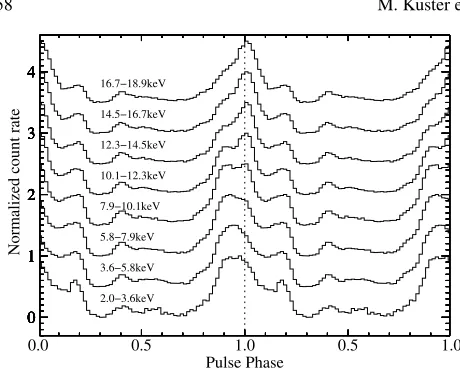
For the following discussion, we use the nomenclature given in Fig. 4 for the various features of the Her X-1 pulse pro-file. Figure 5 shows how the relative strength of these features change with energy. The most distinct variation apparent, is the decreasing flux of the soft leading shoulder with increas-ing energy. This change leads to a double peaked structure
0 200 400 600 800 1000
0.0 0.5 1.0 0.5 1.0
Pulse Phase
Hard Central Peak Soft Leading
Shoulder
Soft Trailing Shoulder
Interpulse
Main Pulse
Count Rate [cts/s]
Fig. 4. Nomenclature for the different features of the Her X-1 pulse profile. This pulse profile is taken from orbit 30 in the energy range of 9.0–13.0 keV.
consisting of the hard central peak and the soft leading shoul-der that clearly can be identified in the energy range 6–12 keV (Deeter et al. 1998).
[image:6.595.298.524.428.593.2]0 1 2 3 4
0.0 0.5 1.0 0.5 1.0
Pulse Phase 2.0−3.6keV
0 1 2 3 4
3.6−5.8keV
0 1 2 3 4
5.8−7.9keV
0 1 2 3 4
7.9−10.1keV
0 1 2 3 4
10.1−12.3keV
0 1 2 3 4
12.3−14.5keV
0 1 2 3 4
14.5−16.7keV
0 1 2 3 4
16.7−18.9keV
[image:7.595.64.294.69.254.2]Normalized count rate
Fig. 5. Energy dependence of the pulse profile. The pulse profile of orbit 31 is shown in eight different energy bands. All profiles are nor-malized to unity. Each profile, except the profile of the energy range 2.0–3.6 keV, is shifted by 0.5 in theydirection relative to the previous profile. Note, the energy-dependent change of the relative intensity of the soft leading shoulder to the hard central peak, which results in a double peaked structure close to pulse phase 1.0. This feature is most pronounced at energies between 10–14 keV.
by strong noise. This implies that during this phase energy-dependent photoelectric absorption is the dominant process. The behavior during orbits 05–09 is very similar to the sit-uation in orbits 10–14 during which the anomalous dip took place, which is presumably caused by cold material located at the outer rim of the accretion disk, crossing the line of sight to the neutron star (Shakura et al. 1999). During the eclipse phase (orbit 21–22) all energy channels are affected by strong noise and no pulsation was detected.
These effects of scattering and photoelectric absorption can also be seen in the behavior of the pulsed fraction with time (Fig. 7). It is clearly visible that Fpulsed increases more rapidly in the high energy bands. At lower energies, the pulsed flux is suppressed towards the beginning of the turn-on, similar to the situation observed during egress of the anomalous dip, where the pulsed flux increases faster at higher energies. At the end of the turn-on, after orbit 23, the pulsed fraction is almost con-stant. Contrary to later phases of the main-on and the turn-off the intrinsic pulse shape does not change significantly over the time of the turn-on. This result is in agreement with earlier find-ings of, e.g., Gruber et al. (1980), Bai (1981), Trümper et al. (1986), or Deeter et al. (1998). The pulse profile observed at the beginning of the turn-on can be interpreted, therefore, as a main-on pulse profile modified by the influence of photoelec-tric absorption and scattering.
5. Simulating pulse variation
To quantify the effects of scattering and photoelectric absorp-tion on the change of the X-ray spectrum and the pulse pro-file shown in Sects. 3 and 4, we now turn to Monte Carlo simulations of the radiation transport of the pulsar’s flux in a scattering medium. For the simulations we assume that the pulse shape seen at the end of the turn-on (orbit 30), is the
intrinsic pulse shape caused by the emission characteristic of the neutron star and is not changing over the time of the turn-on. Furthermore, we assume that the smearing of the pulse pro-file and the change in spectral shape at the beginning of the turn-on are solely caused by scattering and photoelectric ab-sorption in the medium covering the line of sight to the neutron star. With these assumptions we can use the pulse profile ob-served in orbit 30 as a “template” profile and investigate the effects of a scattering and absorbing corona on the pulse shape depending on NHand the size of the scattering region. This is done via Monte Carlo simulations, as described in the follow-ing sections.
5.1. Monte Carlo simulations
Assuming a point source emitting the intensity I(t0) at time t0, the intensity at infinity observed at time t can be written as
I∞(t)= t
−∞G(t,t0)I(t0)dt0 (4) where G(t,t0) is the scattering Green’s function, i.e., the appro-priately normalized solution of the time-dependent equation of radiation transfer through the scattering and absorbing medium for aδ-function pulse of light emitted at time t0.
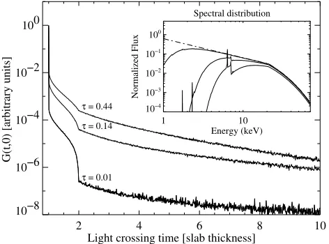
First analytical approaches to determine the Green’s func-tion for scattering in a cold corona were based on the funda-mental method developed by Lightman et al. (1981). Brainerd & Lamb (1987), Kylafis & Klimis (1987), and Kylafis & Phinney (1989) found analytical solutions for G(t,t0) for sim-ple geometries, such as the diffusion of photons out of a spher-ical shell surrounding a central point source. For the general case, analytical results are difficult to obtain and one has to resort to numerical solutions instead. Here, we use a modifi-cation of the linear Monte Carlo code based on the method of weights (Sobol 1991) that we have previously used to com-pute G(t,t0) for the case of a hot Comptonizing plasma (Nowak et al. 1999). In our simulations we consider Compton scattering (using the Klein-Nishina cross section), photoelectric absorp-tion from material of solar abundance using the cross secabsorp-tions of Verner et al. (1996), and fluorescent line emission (using the fluorescence yields of Kaastra & Mewe 1993). We model the propagation of photons through a plane-parallel slab with thickness d and hydrogen column NH(corresponding to a cer-tain optical depth for electron scattering,τes) that is illuminated by a source at infinity. We consider both, neutral and fully ion-ized slabs. Output of the simulation is G(t,t0) as a function of NH, d, and energy band and the angle-dependent photon spectrum of photons leaving the slab. We normalize the time to the light crossing time of the slab.
Obs. 2.0−4.5 keV 4.5−6.5 keV 6.5−9 keV 9−13 keV 13−19 keV
00
0.000.25 0.50 0.75 1.00
02
0.00 0.25 0.50 0.75
03
0.000.25 0.50 0.75
04
0.00 0.25 0.500.75
05
0.000.25 0.50 0.75
09
0.00 0.25 0.500.75
10
0.000.25 0.50 0.75
12
0.00 0.25 0.500.75
13
0.000.25 0.50 0.75
14
0.00 0.25 0.500.75
15
0.00 0.25 0.50 0.75
19
0.00 0.25 0.500.75
20
0.00 0.25 0.50 0.75
21
0.00 0.25 0.500.75
22
0.00 0.25 0.50 0.75
23
0.000.25 0.50 0.75
24
0.00 0.25 0.50 0.75
30
0.000.25 0.50 0.75
0.0 0.5 1.0 0.5 0.0 0.5 1.0 0.5 0.0 0.5 1.0 0.5 0.0 0.5 1.0 0.5 0.0 0.5 1.0 0.5 1.0
[image:8.595.64.507.82.659.2]Pulse Phase
Fig. 6. Evolution of the pulse profile as observed over the time of the turn-on. All profiles are normalized to unity at the maximum of the main pulse, after subtraction of the off-pulse constant flux. Pulse phase 0 is defined as the maximum of the main pulse in the energy band of 13–19 keV.
electron optical depth, the number of diffusing photons in-creases significantly since the mean number of scatterings per photon increases approximately as∼τ2
es. As a consequence, the maximum of G(t,t0) moves towards higher diffusion times, un-til G(t,t0) is dominated by photons scattered multiple times
0 20 40 60
0 5 10
15
20
25 30
Eclipse
Dip
Dip
2.0−4.5 keV
0 20 40 60
0 5 10
15
20
25 30
Eclipse
Dip
Dip
4.5−6.5 keV
0 20 40 60
0 5 10
15 20 25 30
Eclipse
Dip
Dip
6.5−9 keV
0 20 40 60
0
5 10
15 20 25 30
Eclipse
Dip
Dip
9−13 keV
0 20 40 60
50704.0 50704.5 50705.0 50705.5 50706.0 50706.5 50707.0
Time [MJD] 0
5 10
15 20 25 30
Eclipse
Dip
Dip
13−19 keV
[image:9.595.114.514.79.374.2]Percentage of Pulsed Flux
Fig. 7. Pulsed fraction over the time of the turn-on in different energy ranges. To determine the pulsed fraction the pulse profiles have to be smoothed to reduce Poisson noise. The pulsed fraction is given as percentage of the pulsed flux compared to the non pulsed flux.
1 10
Energy (keV) 10−4
10−3
10−2
10−1
100
Normalized Flux
Spectral distribution
2 4 6 8 10
10−8 10−6 10−4 10−2 100
Light crossing time [slab thickness]
G(t,0) [arbitrary units]
τ = 0.01
τ = 0.14
τ = 0.44
Fig. 8. G(t,t0) in the energy range 1.0–70.0 keV for a neutral corona and low optical depths ofτes =0.01 (NH =1.0× 1022 cm−2),τes = 0.14 (NH=1.25×1023cm−2), andτes=0.44 (NH=2.75×1024cm−2). The peak at t = 1 is caused by photons crossing the slab without scattering, the break at t =2 is caused by photons scattering at most one time before leaving the slab. Inset: Spectrum emerging from the slab for the same columns. Note the emergent fluorescent emission lines for the larger optical depths.
band of 2–10 keV. This redistribution effect is the origin of the changing spectral shape with increasing optical depth visible in Fig. 9 (inset). As a consequence, the cut-offenergy moves to-wards lower energies and a bump at energies between 1–5 keV arises. For even larger optical depths,τes > 10, this bump
1 10
Energy (keV) 10−4
10−3
10−2
10−1
100
Normalized Flux
Spectral distribution
2 4 6 8 10
10−5 10−4 10−3 10−2 10−1 100 101
Light crossing time [slab thickness] G(t,0) [arbitrary units] τ = 1 τ = 2
τ = 5
τ = 10
τ = 30
Fig. 9. G(t,t0) for the same spectral distribution as shown in Fig. 8 but for a fully ionized medium and higher optical depths.
slowly vanishes and the flux above 6 keV decreases rapidly. The overall spectral shape is then given by the left most spec-trum shown in the top panel of Fig. 9.
Considering a neutral medium, absorption plays the domi-nant role over the temporal effects of Compton scattering. For a neutral medium withτes 1, almost all flux below 10 keV is suppressed1. At such optical depths the effects caused by 1 For material with solar abundance, the photoionization cross
[image:9.595.64.300.420.595.2] [image:9.595.324.559.420.598.2]1.0
0.0 0.5
τ=0.5
1.0
0.0 0.5
τ=0.5
1.0
0.0 0.5
τ=0.5
1.0
0.0 0.5
τ=0.5
Normalized Flux
0.0 0.5
τ=1.0
0.0 0.5
τ=1.0
0.0 0.5
τ=1.0
0.0 0.5
τ=1.0
0.0 0.5
τ=1.5
0.0 0.5
τ=1.5
0.0 0.5
τ=1.5
0.0 0.5
τ=1.5
0.0 0.5
τ=2.0
0.0 0.5
τ=2.0
0.0 0.5
τ=2.0
0.0 0.5
τ=2.0
0.0 0.5
τ=2.5
0.0 0.5
τ=2.5
0.0 0.5
τ=2.5
0.0 0.5
τ=2.5
0.0 0.5
τ=3.0
0.0 0.5
τ=3.0
0.0 0.5
τ=3.0
0.0 0.5
τ=3.0
0.0 0.5
τ=5.0
0.0 0.5 1.0 0.5 1.0
Pulse Phase 0.0
0.5
τ=5.0
0.0 0.5 1.0 0.5 1.0
Pulse Phase 0.0
0.5
τ=5.0
0.0 0.5 1.0 0.5 1.0
Pulse Phase 0.0
0.5
τ=5.0
0.0 0.5 1.0 0.5 1.0
[image:10.595.32.271.83.449.2]Pulse Phase
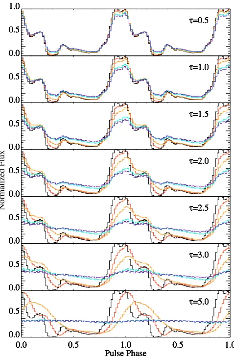
Fig. 10. Her X-1 pulse profile of orbit 30 (black) transmitted by a fully ionized scattering medium. The electron optical depth varies from top to bottom from τes = 0.5 to τes = 5.0. In addition, for each optical depth value the thickness d of the scattering medium is set to 0.02 (red), 0.02 (yellow), 0.2 (blue), and 0.4 times (dark blue) the light crossing time of the slab.
diffusion time are still negligible since the mean number of scatterings per photon is close to unity. Thus, to achieve notice-able changes in beam shape a high fraction of ionized material is needed. On the other hand a high fraction of neutral material only weakly alters the beam shape but reduces the flux at low energies.
Figure 10 demonstrates the influence of a fully ionized scat-tering medium on the pulse shape of Her X-1 for different val-ues ofτesand a variable thickness of the slab. It is obvious that for large optical depth values (τes >3), even a thin scattering layer (d<0.1) is sufficient to completely hide the pulse. In ad-dition the structure of the pulse profile is steadily “washed-out” to an almost sinusoidal pulse shape. Forτes <1.5 the profile’s substructure (soft trailing shoulder) is still apparent even for high values of d. Note especially the shift in pulse phase, which is pronounced in the modified pulse profile forτes>2.0. This phase shift corresponds to the shift of the maximum of G(t,t0) apparent in Fig. 9.
5.2. Analysis of the pulse profile
To simulate the variation of the pulse profile during the turn-on we calculated G(t,t0) for the same energy ranges we used in Sect. 4 and each RXTE orbit for two cases:
1. Gn(t,t0) for a neutral corona, with NH,n≈NHof the spectral analysis for each single orbit.
2. Gion(t,t0) for a completely ionized corona with 1.0 × 1022cm−2≤N
H,es≤9.5×1024cm−2.
The Green’s functions Gn(t,t0) and Gion(t,t0) can then be compared directly with the spectral model given by Eq. (2). Following the notation introduced in Sect. 3.1, Gion(t,t0) corre-sponds to the model component MC I and Gn(t,t0) to the model component MC II used for the spectral analysis. For a medium where a fraction f is fully ionized, the total Green’s function is given by G(t,t0)=(1−f ) Gion(t,t0)+f Gn(t,t0). Using a fixed Gn(t,t0) with the respective NH,nfor each orbit from the spectral analysis and variable Gion(t,t0), we can simulate pulse profiles an observer located at infinity would see, by applying Eq. (4) to the “template” pulse profile. As mentioned above, the time scale of the simulated light curves is normalized to the thick-ness of the corona, i.e., t−t0is measured in units of the light crossing time of the slab. Therefore, Green’s functions for dif-ferent values of d can be obtained by simply rescaling the time. For our analysis we chose d between 0.1 and 6 light seconds, appropriate for the dimension of the accretion disk in Her X-1 with rin ∼108cm and rout ∼ 1011cm (Cheng et al. 1995). To obtain a proper flux normalization, the integrated flux of the profile of orbit 30 was set to unity. All other simulated pulse profiles are normalized relative to this flux. From the spectral fitting of the partial covering model to the observed spectra, the parameters of the spectral model components MC I and MC II are known. By integrating the differential photon flux of the model spectra over the specific energy bands of Fig. 6, the total flux per energy range can be calculated. Using the integrated photon flux both Green’s functions, Gn(t,t0) and Gion(t,t0), can then be normalized to the observed flux according to
t1
t0 ∞
0
R(h,E)Nph(E,t) dE dt= t
−∞GE1,E2(t,t
) dt (5)
where Nph(E) is the differential photon flux and R(h,E) the de-tector response matrix. Finally we performed aχ2 minimiza-tion fit of simulated to observed pulse profiles as shown in Fig. 6 for each single RXTE orbit. The different energy ranges were fitted simultaneously. This procedure allows us to deter-mine NH,es, and d as well as their uncertainty.
As an example, the results of the fit of simulated to
Orbit 05
0 2000 4000 6000 8000
Flux [counts]
2.0 - 4.5 keV
0.8 0.9 1.0 1.1 1.2
Data/Fit
0.0
Pulse Phase 0.5 1.0 1.5 0.0
4.5 - 6.5 keV
0.5 1.0 1.5 0.0 6.5 - 9.0 keV
0.5 1.0 1.5 0.0 9.0 -13.0 keV
0.5 1.0 1.5 0.0
13.0 -19.0 keV
0.5 1.0 1.5 0.0
Orbit 06
0 2000 4000 6000 8000 10000
Flux [counts]
2.0 - 4.5 keV
0.8 0.9 1.0 1.1 1.2
Data/Fit
0.0
Pulse Phase 0.5 1.0 1.5 0.0
4.5 - 6.5 keV
0.5 1.0 1.5 0.0 6.5 - 9.0 keV
0.5 1.0 1.5 0.0 9.0 -13.0 keV
0.5 1.0 1.5 0.0
13.0 -19.0 keV
0.5 1.0 1.5 0.0
Orbit 08
0 2000 4000 6000 8000
Flux [counts]
2.0 - 4.5 keV
0.8 0.9 1.0 1.1 1.2
Data/Fit
0.0
Pulse Phase 0.5 1.0 1.5 0.0
4.5 - 6.5 keV
0.5 1.0 1.5 0.0 6.5 - 9.0 keV
0.5 1.0 1.5 0.0 9.0 -13.0 keV
0.5 1.0 1.5 0.0
13.0 -19.0 keV
0.5 1.0 1.5 0.0
Orbit 09
0 2000 4000 6000 8000
Flux [counts]
2.0 - 4.5 keV
0.8 0.9 1.0 1.1 1.2
Data/Fit
0.0
Pulse Phase 0.5 1.0 1.5 0.0
4.5 - 6.5 keV
0.5 1.0 1.5 0.0 6.5 - 9.0 keV
0.5 1.0 1.5 0.0 9.0 -13.0 keV
0.5 1.0 1.5 0.0
13.0 -19.0 keV
0.5 1.0 1.5 0.0
Orbit 15
0 5.0•103 1.0•104 1.5•104 2.0•104 2.5•104 3.0•104
Flux [counts]
2.0 - 4.5 keV
0.8 0.9 1.0 1.1 1.2
Data/Fit
0.0
Pulse Phase 0.5 1.0 1.5 0.0
4.5 - 6.5 keV
0.5 1.0 1.5 0.0 6.5 - 9.0 keV
0.5 1.0 1.5 0.0 9.0 -13.0 keV
0.5 1.0 1.5 0.0 13.0 -19.0 keV
0.5 1.0 1.5 0.0
Orbit 24
0 5.0•103 1.0•104 1.5•104 2.0•104
Flux [counts]
2.0 - 4.5 keV
0.8 0.9 1.0 1.1 1.2
Data/Fit
0.0
Pulse Phase 0.5 1.0 1.5 0.0
4.5 - 6.5 keV
0.5 1.0 1.5 0.0 6.5 - 9.0 keV
0.5 1.0 1.5 0.0 9.0 -13.0 keV
0.5 1.0 1.5 0.0 13.0 -19.0 keV
[image:11.595.64.541.87.645.2]0.5 1.0 1.5 0.0
[image:11.595.311.540.91.499.2]Fig. 11. Fit of simulated pulse profiles to observed pulse profiles for the selected observations (compare Fig. 6). The solid line represents the count rate of the observed pulse profile of the indicated orbit, and the dashed line represents the simulated best-fit pulse profile. The residuals of the fits are given at the bottom. All energy bands are fitted simultaneously.
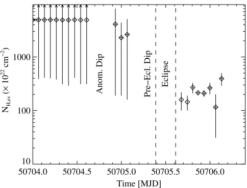
Figure 12 shows the overall development of the electron optical depth over the full turn-on. In the figure we giveτesin terms of the electron column depth, NH,es, to enable a direct comparison with the results of the spectral fitting. During the early phases of the turn-on, NH,esis very high and the absorb-ing medium is Compton thick. For the later observations, NH,es
10 100 1000
NH,es
(
×
10
22 cm −2 )
Time [MJD]
50704.0 50704.5 50705.0 50705.5 50706.0
Eclipse
Pre−Ecl. Dip
[image:12.595.32.274.82.266.2]Anom. Dip
Fig. 12. NH,es as a function of time determined with the method of pulse profile fitting as described in the text. The error bars are at the 1σconfidence level.
electron column deduced from our Monte Carlo simulations is significantly higher than the column deduced from spectral fitting. Given the explorative character of the Monte Carlo sim-ulations and the simplifications introduced in the model, this is not unexpected. For example, our assumption of the scat-tering medium being a mixture of either completely neutral or completely ionized is certainly an oversimplification, as is the assumption of a slab geometry. On the other hand, as we will show below, despite these simplifications the overall trend of NH,esis in agreement with the common models for the 35 day turn-on and thus reduces the ambiguities from the spectral de-composition.
6. Conclusion and discussion
In this paper we have shown that the evolution of the X-ray spectrum and pulse profile during the 35 day turn-on of Her X-1 can be explained by invoking a varying contribution of scattered and heavily absorbed photons to the observed data (Sects. 3 and 5). Using Monte Carlo simulations, in Sect. 5 we showed that the observed behavior of these components ap-pears to be consistent with the results of pulse profile analysis with theoretical Green’s functions for the scattering and pho-toelectric absorption in the accretion disk. Despite the existing limitations, such as modeling the accretion disk rim by a sim-ple slab with uniform density or modeling the scatterer as either fully ionized or neutral, the methods applied here show that the distinct contributions to the final pulse profile and spectrum can in principle be separated by making use of the smearing of the pulse profile caused by the scattering in the plasma. Our results confirm earlier work based on X-ray spectral analysis alone on the nature of the turn-on of the 35 day cycle and on the na-ture of the accretion disk of Her X-1 (Davison & Fabian 1977; Parmar et al. 1980; Becker et al. 1977; Burwitz et al. 2001). Our analysis yields an optical depth ofτes ≈3–10 for the scatter-ing medium which is necessary to explain the observed smear-ing of the pulse profile. Such optical depths are consistent with
coronal models of neutron stars in LMXRBs (e.g., Miller 2000, and references therein).
The behavior summarized above can be explained by a sim-ple geometric model that takes into account the outer rim of an accretion disk that opens the line of sight to the neutron star and the influence of a hot accretion disk corona sandwich-ing the accretion disk. Figure 13 shows the positions of the accretion disk, the disk corona, and the location of the ob-server are shown for different times of the turn-on. The ob-served PCA spectra corresponding to the phases of the turn-on and the unfolded spectral model compturn-onents for the energy range 3≤E ≤12 keV are shown in the right panel of Fig. 13. The individual components of the spectral model are shown separately.
At the start of the turn-on, Thomson scattered radiation from the corona, which is partially absorbed, dominates the observed spectrum. The topmost image of Fig. 13 “Beginning of turn-on” illustrates the orientation of the disk and the loca-tion of the observer relative to the disk for this time. Photons following beam A, marked by a dashed line, are scattered in the corona and partially absorbed in the disk rim (beam C). The direct view to the neutron star at this time is still blocked and photons following beam B cannot reach the observer. The corresponding spectra are those observed in orbits 00 and 04. Since the scattered spectral model component MC I dominates the observed spectral flux, only a small fraction of absorbed flux can be detected. As a result, the total observed spectrum,
which is the sum of all model components, shows only a weak signature of absorption and low values of NHare measured. On the other hand, however, those scattered photons which finally reach the observer have undergone many scattering events such that the pulse profile is heavily distorted until orbit 06. In the pulse profile fitting, this phase of the turn-on will therefore be characterized by large values of NH,es.
As soon as the disk starts to open the line of sight to the neu-tron star (indicated by the downward moving disk in the image “Mid of Turn-On” of Fig. 13), the visible parts of the corona in-crease and consequently the observed flux in MC I inin-creases as well. In parallel, the apparent absorbed flux increases, because the disk becomes more and more transparent for photons scat-tered in the corona (beam C). Around the mid point of the turn-on, the outer disk rim starts to become optically thin for pho-tons directly coming from the neutron star following beam D (“Mid of turn-on”). As a consequence the flux in component MC II (the ratio C in Fig. 3) rises more rapidly compared to the flux of MC I. Since MC II determines the curvature of the total observable spectrum, NHapparently increases. Since the pulse profile due to MC II expected to be far less smeared, pulse profile fitting during this episode will shown a decrease of the overall NH,es. During the further evolution the contribution of MC II continues to increase until it dominates the spectrum. This event takes place right after the turning point in the track of NHshown in Fig. 3a.
Observer Observer Observer
Outer Accretion Disk Rim
10−2
10−3
Orbit 00
10−1
10−2
10−3
Orbit 04
10−1
10−2
10−3
Orbit 06
10−1
10−2
10−3
Orbit 08
10−1
10−2
10−3
Orbit 09
10−1
10−2
10−3
Orbit 17
10−1
10−2
10−3
Orbit 27
3 5 7 10
Channel Energy [keV]
E f(E) [keV ph/cm
2/s/keV]
Disk Corona
Neutron Star Mid of Turn−On
Disk Corona
Neutron Star Disk Corona Beginning of Turn−On
Scattered Radiation
Neutron Star
After Turn−On
C
A
D
B
[image:13.595.84.540.83.582.2]A B
Fig. 13. Schematic view of the outer accretion disk rim (blue), the accretion disk corona (grey), and the neutron star for three different times during the turn-on (not to scale). Right panel: Unfolded PCA spectra and the components of the spectral model for selected orbits. The following components are shown: observed spectrum (solid line), spectral model component MC I (dotted line) and MC II (dashed line), and the Fe line.
larger amount of photons from the inner parts of the accretion disk close to the neutron star reach the observer. Finally, at the end of the turn-on, the neutron star is directly visible when the main-on starts.
In summary, models as the one outlined above seem to be successful in describing the overall features of the 35 day turn-on of Her X-1. We note, however, that our results in Sect. 5 also show that for very high columns, the separation into two com-ponents fails due to low counting statistics during early phases of the turn-on although the overall picture stays consistent. The success of the analysis presented here, however, is a first step
towards self-consistently modeling both, the spectral evolution and the timing behavior of Her X-1. Further refinements of the method are still possible, e.g., when taking the absolute phase shift of the observed pulse profile into account and by using more realistic geometries.
Appendix A: Results of the spectral analysis
Table A.1. Results of the spectral fitting to the Her X-1 turn-on data with all parameters set free, except the parameters where no errors are given for and the power law indexαwhich was kept fix atα=1.068.
Obs. NH C APL Ecut Efold EFe σFe ALine Ecyc σcyc τcyc χ2/d.o.f.
1022cm2 10−3 keV keV keV keV 10−4 keV keV
00 44.73+3.17
−7.24 2.14+ 0.14
−0.13 4.2+ 0.2
−0.2 18.16+ 3.46
−2.21 15.4+ 16.6
−7.4 6.69+ 0.11
−0.14 0.77 4.6+ 0.8
−0.7 39.7 5.10 0.50+
2.58
−0.50 77.3/103
01 47.34+6.14
−4.28 2.19+ 0.15
−0.12 5.0+ 0.2
−0.2 18.24+ 2.21
−1.57 9.5+ 5.6
−3.3 6.68+ 0.11
−0.11 0.77 5.3+ 0.7
−0.7 39.7 5.10 0.00+
2.09
−0.00 102.4/103
02 56.26+4.13
−3.65 3.16+ 0.16
−0.15 6.1+ 0.2
−0.2 18.42+ 3.01
−1.69 20.0+ 10.3
−7.5 6.60+ 0.09
−0.09 0.77 7.6+ 0.8
−0.8 39.7 5.10 1.31+
1.38
−1.19 163.7/103
03 67.38+1.07
−7.67 3.57+ 0.16
−0.15 8.1+ 0.2
−0.2 20.57+ 2.76
−2.69 14.3+ 8.8
−7.7 6.57+ 0.07
−0.07 0.77 11.4+
0.9
−0.9 39.7 5.10 1.61+
1.71
−1.61 134.5/103
04 77.35+1.81
−2.96 4.49+ 0.14
−0.15 12.2+ 0.2
−0.2 19.98+ 1.45
−1.63 11.6+ 3.9
−2.8 6.42+ 0.06
−0.02 0.77 15.0+
1.1
−1.0 39.7 5.10 0.46+
0.82
−0.46 165.3/103
05 75.17+1.62
−2.39 6.01+ 0.14
−0.17 15.2+ 0.2
−0.2 21.53+ 1.08
−1.08 13.6+ 2.8
−2.8 6.54+ 0.07
−0.08 0.77 16.5+
1.4
−1.3 39.7 5.10 0.91+
0.56
−0.56 198.9/103
06 61.37+1.46
−1.23 7.15+ 0.13
−0.15 17.4+ 0.3
−0.3 21.05+ 0.92
−0.98 14.5+ 2.4
−2.2 6.70+ 0.10
−0.10 1.00+ 0.13
−0.02 13.4+ 1.8
−1.8 39.7 5.10 1.25+
0.52
−0.47 142.7/103
07 54.84+1.35
−1.26 7.70+ 0.17
−0.16 17.7+ 0.4
−0.4 21.01+ 0.78
−0.88 12.0+ 2.2
−2.0 6.71+ 0.09
−0.12 1.00+ 0.00
−0.09 17.7+ 2.7
−3.0 39.7 5.10 0.41+
0.51
−0.41 122.2/102
08 65.75+2.77
−0.80 9.94+ 0.31
−0.20 14.3+ 0.3
−0.3 21.07+ 0.86
−0.93 12.9+ 2.2
−1.9 6.68+ 0.12
−0.11 0.98+ 0.13
−0.02 14.7+ 2.3
−1.7 39.7 5.10 0.69+
0.46
−0.40 119.8/102
09 52.66+1.27
−1.39 8.37+ 0.17
−0.21 17.6+ 0.4
−0.4 21.56+ 1.04
−1.10 11.3+ 2.6
−2.5 6.67+ 0.13
−0.15 1.00+ 0.00
−0.10 17.1+ 3.0
−3.0 39.7 5.10 0.77+
0.67
−0.68 135.1/102
15 25.36+0.70
−0.94 5.75+ 0.13
−0.13 25.5+ 0.8
−1.4 21.24+ 0.39
−0.41 12.9+ 1.0
−1.0 6.55+ 0.10
−0.10 1.00+ 0.00
−0.60 31.6+ 4.2
−4.6 39.7 5.10 1.02+
0.22
−0.22 108.2/101
16 11.91+2.30
−2.32 0.70+ 0.25
−0.10 98.3+ 1.5
−14.2 21.18+ 0.46
−0.47 12.6+ 1.1
−1.1 6.55+ 0.10
−0.11 0.71+ 0.18
−0.14 39.2+ 6.8
−5.2 39.7 5.10 0.80+
0.25
−0.24 93.1/101
17 4.74+0.42
−0.48 1.00 85.0+
0.4
−0.4 21.24+ 0.46
−0.48 12.4+ 1.1
−1.1 6.60+ 0.11
−0.11 0.72+ 0.18
−0.15 41.2+ 6.6
−5.5 39.7 5.10 0.77+
0.26
−0.26 98.9/102
18 5.17+0.45
−0.46 1.00 85.3+
0.4
−0.4 21.13+ 0.43
−0.44 12.0+ 1.0
−1.0 6.63+ 0.11
−0.12 0.78+ 0.18
−0.16 41.2+ 6.8
−5.7 39.7 5.10 0.76+
0.25
−0.25 84.4/102
23 6.49+0.37
−0.50 1.00 100.5+
3.2
−0.4 21.91+ 0.58
−0.57 10.8+ 2.2
−1.0 6.53+ 0.11
−0.13 0.75+ 0.19
−0.13 50.4+ 8.3
−6.9 40.6+ 0.8
−0.9 5.10 2.39+
3.92
−1.41 108.7/101
24 5.23+0.48
−0.38 1.00 103.5+
0.7
−0.5 20.77+ 0.67
−0.71 13.7+ 1.6
−1.3 6.59+ 0.09
−0.10 0.70+ 0.18
−0.15 53.3+ 8.7
−7.1 39.2+ 1.1
−1.0 3.34+ 1.90
−1.45 1.48+ 0.96
−0.45 122.7/100
25 4.30+0.43
−0.38 1.00 104.8+
0.7
−0.5 21.21+ 0.53
−0.48 13.4+ 1.5
−1.1 6.62+ 0.09
−0.10 0.71+ 0.17
−0.15 52.8+ 8.1
−7.2 39.7+ 1.0
−0.9 5.37+ 2.13
−1.50 1.16+ 0.27
−0.24 117.7/100
26 4.31+0.40
−0.38 1.00 104.7+
0.6
−0.4 22.06+ 0.38
−0.34 11.3+ 1.1
−0.9 6.64+ 0.08
−0.10 0.78+ 0.17
−0.13 58.8+ 8.6
−6.7 40.0+ 1.2
−1.2 5.18+ 2.85
−2.32 0.71+ 0.20
−0.17 106.6/100
27 4.58+0.41
−0.39 1.00 110.9+
0.7
−0.5 21.01+ 0.35
−0.36 12.8+ 1.3
−0.9 6.68+ 0.09
−0.10 0.75+ 0.17
−0.14 57.2+ 8.4
−7.0 40.4+ 0.9
−0.9 5.16+ 2.33
−1.69 0.95+ 0.19
−0.17 110.9/100
28 4.36+0.36
−0.35 1.00 110.5+
3.9
−0.7 21.19+ 0.29
−0.29 12.2+ 0.8
−0.6 6.65+ 0.08
−0.09 0.79+ 0.17
−0.15 61.9+ 7.9
−7.5 39.1+ 0.8
−0.8 4.70+ 1.81
−1.33 0.83+ 0.16
−0.15 114.6/100
29 4.24+0.36
−0.31 1.00 116.1+
0.7
−0.6 21.40+ 0.33
−0.31 12.1+ 1.0
−0.6 6.68+ 0.08
−0.10 0.83+ 0.18
−0.16 65.8+ 7.8
−8.2 39.7+ 1.0
−1.0 5.59+ 3.31
−1.55 0.71+ 0.14
−0.13 114.5/100
30 4.55+0.34
−0.41 1.00 118.3+
0.7
−0.5 21.14+ 0.39
−0.37 12.7+ 1.2
−0.9 6.67+ 0.08
−0.08 0.77+ 0.03
−0.15 64.3+ 6.4
−6.9 39.5+ 0.7
−0.7 5.25+ 1.92
−1.48 1.05+ 0.20
−0.19 119.7/100
31 3.48+0.37
−0.37 1.00 116.6+
0.5
−0.4 21.37+ 0.44
−0.46 11.6+ 0.7
−0.7 6.59+ 0.07
−0.08 0.77+ 0.03
−0.13 71.2+ 7.1
−7.5 40.5+ 0.7
−0.7 1.00+ 6.25
−0.00 1.97+ 0.99
−1.39 95.8/100
NH: hydrogen column density, C: relative ratio of absorbed and scattered radiation to the unaffected radiation, APL: power law normaliza-tion, (photons cm−2s−1keV−1
Table A.2. Results of the spectral fitting to the Her X-1 turn-on data for the following parameters: NH, C, APL, and ALine.
Obs. NH C APL ALine χ2/d.o.f.
1022cm2 10−3 10−4
00 35.98+7.60
−1.93 2.10+ 0.16
−0.15 4.2+ 0.2
−0.2 3.8+ 0.6
−0.6 83.9/108 01 42.20+6.44
−2.63 2.13+ 0.14
−0.13 4.9+ 0.2
−0.2 4.1+ 0.6
−0.6 112.4/108
02 62.80+4.71
−3.65 3.59+ 0.23
−0.21 6.1+ 0.2
−0.2 10.7+ 1.1
−1.1 162.3/108 03 67.61+4.17
−2.60 3.97+ 0.20
−0.19 8.0+ 0.2
−0.2 14.3+ 1.1
−1.1 131.1/108 04 83.92+0.33
−4.83 5.11+ 0.21
−0.19 11.8+ 0.2
−0.2 20.4+ 1.4
−1.4 151.1/108
05 82.43+1.91
−2.03 7.61+ 0.28
−0.28 13.9+ 0.3
−0.3 35.3+ 2.5
−2.5 115.5/108 06 66.27+1.65
−1.65 8.19+ 0.26
−0.25 16.6+ 0.3
−0.3 31.0+ 3.6
−3.7 130.4/108 07 55.18+1.14
−1.57 7.80+ 0.18
−0.17 17.7+ 0.3
−0.4 19.0+ 2.8
−2.8 138.9/108
08 67.47+0.74
−2.29 10.10+ 0.25
−0.26 14.2+ 0.3
−0.3 16.0+ 2.5
−2.5 135.3/108 09 53.46+1.84
−1.09 8.64+ 0.22
−0.21 17.5+ 0.1
−0.4 22.2+ 2.3
−3.8 154.4/108 15 24.02+0.81
−0.52 6.00+ 0.30
−0.24 24.4+ 1.0
−1.1 23.0+ 2.8
−2.8 145.7/107
16 8.13+4.50
−0.90 0.77+ 0.50
−0.10 94.0+ 1.0
−2.2 34.0+ 3.7
−3.4 128.7/107 17 4.84+0.37
−0.44 1.00+ 0.00
−0.00 85.5+ 0.4
−0.4 39.6+ 3.9
−3.9 135.6/108 18 5.34+0.43
−0.41 1.00+ 0.00
−0.00 85.9+ 0.4
−0.4 38.5+ 3.9
−3.9 105.6/108
23 6.72+0.54
−0.35 1.00+ 0.00
−0.00 101.3+ 0.6
−0.5 48.7+ 5.1
−5.0 121.9/108
24 5.30+0.43
−0.31 1.00+ 0.00
−0.00 104.2+ 0.6
−0.5 46.6+ 4.9
−4.8 144.1/108 25 4.41+0.40
−0.38 1.00+ 0.00
−0.00 105.2+ 4.1
−0.4 51.2+ 4.9
−4.9 137.4/108
26 4.55+0.35
−0.42 1.00+ 0.00
−0.00 105.4+ 0.5
−0.4 55.2+ 4.7
−4.7 129.3/108
27 4.72+0.35
−0.42 1.00+ 0.00
−0.00 111.4+ 0.5
−0.4 54.8+ 4.8
−4.8 134.8/108 28 4.47+0.37
−0.39 1.00+ 0.00
−0.00 111.2+ 0.5
−0.5 58.0+ 5.0
−5.0 140.9/108 29 4.33+0.36
−0.40 1.00+ 0.00
−0.00 116.6+ 0.5
−0.5 63.8+ 5.4
−5.4 173.8/108
30 4.75+0.35
−0.43 1.00+ 0.00
−0.00 156.7+ 17.1
−14.1 65.1+ 6.4
−5.8 150.2/108 31 3.70+0.40
−0.38 1.00+ 0.00
−0.00 117.4+ 0.6
−0.5 70.7+ 5.8
−5.8 102.9/108
NH: hydrogen column density, C: relative ratio of absorbed and scattered radiation to the unaffected radiation, APL: power law normalization (photons cm−2s−1keV−1at 1 keV), A
Line: line normalization (photons cm−2s−1in the line), the following parameters were fixed: the Gaussian emission line was fixed at 6.45 keV with a widthσof 0.45 keV, the cut offenergy Ecutat 21.5 keV, the folding energy Efoldat 14.1 keV, the power law indexαat 1.068, and the cyclotron energy Ecyc at 39.4 keV with a width of 5.1 keV. Uncertainties are at 90% confidence level for one interesting parameter (∆χ2=2.71).
References
Arnaud, K., & Dorman, B. 2002, Xspec, An X-ray Spectral Fitting Package, User’s Guide for version 11.2.x, Tech. rep., HEASARC – Laboratory for High Energy Astrophysics – NASA/GSFC, available at http://heasarc.gsfc.nasa.gov/ docs/xanadu/xspec/manual/manual.html
Bai, T. 1981, ApJ, 243, 244
Becker, R. H., Boldt, E. A., Holt, S. S., et al. 1977, ApJ, 214, 879 Boyd, P., Still, M., & Corbet, R. 2004, The Astronomer’s Telegram,
307, 1
Brainerd, J., & Lamb, F. K. 1987, ApJ, 317, L33
Burwitz, V., Dennerl, K., Predehl, P., & Stelzer, B. 2001, in Two Years of Science with Chandra, Abstracts from the Symposium held in Washington, DC, 5–7 September, 2001
Cheng, F. H., Vrtilek, S. D., & Raymond, J. C. 1995, ApJ, 452, 825
Coburn, W., Heindl, W. A., Wilms, J., et al. 2000, ApJ, 543, 351 Dal Fiume, D., Orlandini, M., Cusumano, G., et al. 1998, A&A, 329,
41
Davison, P. J. N., & Fabian, A. C. 1977, MNRAS, 178, 1
Deeter, J. E., Scott, D. M., Boynton, P. E., et al. 1998, ApJ, 502, 802
Giacconi, R., Gursky, H., Kellogg, E., et al. 1973, ApJ, 184, 227 Gruber, D. E., Matteson, J. L., Nolan, P. L., et al. 1980, ApJ, 240,
L127
Kaastra, J. S., & Mewe, R. 1993, A&AS, 97, 443 Katz, J. 1973, Nature Physical Science, 246, 87
Kuster, M., Wilms, J., Blum, S., et al. 1999, Astrophys. Lett. Comm., 38, 161
Kylafis, N. D., & Klimis, G. S. 1987, ApJ, 323, 678
Kylafis, N. D., & Phinney, E. S. 1989, in Timing Neutron Stars, ed. H. Ögelman, & E. P. J. van den Heuvel (Dordrecht: Kluwer), NATO ASI, Vol. C262, 731
Leahy, D. A. 2004, Astron. Nachr., 325, 205
Lightman, A. P., Lamb, D. Q., & Rybicki, G. B. 1981, ApJ, 248, 738 Maloney, P., & Begelman, M. C. 1997, ApJ, 491, L43
Miller, M. C. 2000, ApJ, 537, 342
Nowak, M. A., Wilms, J., Vaughan, B. A., Dove, J. B., & Begelman, M. C. 1999, ApJ, 515, 726
Oosterbroek, T., Parmar, A. N., Orlandini, M., et al. 2001, A&A, 375, 922
Parmar, A. N., Sanford, P. W., & Fabian, A. C. 1980, MNRAS, 192, 311
Parmar, A. N., Pietsch, W., McKechnie, S., et al. 1985, Nature, 313, 119
Parmar, A. N., Oosterbroek, T., dal Fiume, D., et al. 1999, A&A, 350, L5
Schandl, S., & Meyer, F. 1994, A&A, 289, 149
Schandl, S., Staubert, R., & König, M. 1997, in Proc. of the Fourth Compton Symp., AIP Conf. Proc., 410, 763
Scott, D. M., & Leahy, D. A. 1999, ApJ, 510, 974
Scott, D. M., Leahy, D. A., & Wilson, R. B. 2000, ApJ, 539, 392
Shakura, N. I., Postnov, K. A., & Prokhorov, M. E. 1998, A&A, 331, L37
Shakura, N. I., Prokhorov, M. E., Postnov, K. A., & Ketsaris, N. A. 1999, A&A, 348, 917
Sobol, I. M. 1991, Die Monte Carlo Methode, 4th ed. (Berlin: Deutscher Verlag der Wissenschaften), engl. transl.: The Monte Carlo Method (Chicago: Univ. Chicago Press), 1974
Tananbaum, H., Gursky, H., Kellogg, E. M., et al. 1972, ApJ, 174, L143
Trümper, J., Kahabka, P., Ögelman, H., Pietsch, W., & Voges, W. 1986, ApJ, 300, L63
Verner, D. A., Ferland, G. J., Korista, K. T., & Yakovlev, D. G. 1996, ApJ, 465, 487
Vrtilek, S. D., & Cheng, F. H. 1996, ApJ, 465, 915
Vrtilek, S. D., Mihara, T., Primini, F. A., et al. 1994, ApJ, 436, L9 Wilms, J., Allen, A., & McCray, R. 2000, ApJ, 542, 914
![Fig. 3. From top to bottom:of the iron line a) NH [1022cm−2], b) ratio between the model component MC II and MC I as defined in Eq](https://thumb-us.123doks.com/thumbv2/123dok_us/9778103.478869/6.595.298.524.428.593/fig-iron-line-nh-ratio-model-component-dened.webp)