Munich Personal RePEc Archive
A Historical Retrieval of the Methods
and Functions of Monetary Policy
Hassan, Sherif Maher
Center for Near and Middle Eastern Studies (CNMS), Philipps
universität-Marburg, Germany, Suez Canal university, Ismailia,
Egypt
2016
A Historical Retrieval of the Methods and Functions of
Monetary Policy
SHERIF’S DEDICATION
To my fathers
’
soul
TABLE OF CONTENTS
Introduction 5
1.
The evolution of monetary policy 7
1-1. A historical review of the literature 7
1-2. Schools of thinking: waves and counter waves 9 1-2-1. David Hume 9
1-2-2. David Ricardo 10 1-2-3. Keynesians 10 1-2-4. Austrians 20 1-2-5. Monetarism 28
1-2-6. Neo classical-Keynesian synthesis 40 1-2-7. New neo classical synthesis 56 1-3. Connecting the dots 58
2.
The theory of optimal monetary policy 61
2-1. Monetary Transmission Mechanisms (MTMs) 612-1-1. Interest rate channel 61 2-1-2. Exchange rate channel 62 2-1-3. Asset price channel 64 2-1-4. Credit channel 65 2-1-5. Expectations channel 66
2-2. Theory of optimal monetary policy and inflation targeting 67 2-2-1. The need for a new nominal anchor 67
2-2-2. inflation targeting prerequisites 72 2-2-3. How does inflation targeting work? 73
2-2-4. How does inflation targeting come in line with the theory of optimal monetary policy? 75
3.
A review of monetary policy in Egypt 78
3-1. A glimpse of the Egyptian monetary policy 78 3-2. ERSAP (1990-1996) 823-2-1. Monetary policy reforms 83 3-2-2. Inflation under ERSAP 85 3-3. Transitional era (1996-2005) 91
3-3-1. CBE market instruments 93 3-3-2. Internal and external shocks 96 3-3-3. Inflation during the transitional era 98 3-4. Towards inflation targeting (2005-2010) 102
3-4-2. What are still needed for the successful implementation of inflation targeting in Egypt? 107
3-4-3. Guidelines and recommendations 111 3-5. Connecting the dots 113
Introduction
There exists a broad implicit agreement that steering the monetary policy has important consequences for the whole economy (Friedman, 1968). This book uses topic classification to present a historical retrieval of the main theories and applications of the monetary policy within different schools of economic thinking and across history. From Humes‘ automatic price-species flow in the 17th century, to the Keynesians, Monetarists and Austrians perspectives of the monetary dynamics in the beginning of the 19th century.
The second chapter provides a general overview about how the monetary authority can fine tune monetary indicators in response to business cycle shocks. This part will discuss the monetary transmission mechanisms that represent the different means of interaction between monetary tools together and their impact on the real economy. In this context, the concept of inflation targeting will be elaborated in details while explaining its main institutional and economic prerequisites.
Chapter one: the Evolution of Monetary Policy
1-1. A Historical Review of the Literature
My starting point is Blanchard‘s and Woodford‘s surveys of the history of macroeconomics
written on the occasion of the turn of the century. Blanchard (2000) divided the history of macroeconomics into three stages: pre-1940, a period of exploration, from 1940 to 1980, a period of consolidation and since 1980, a new period of consolidation emerged. On contrary, Woodford (1999) found it useful to structure his account on the idea of revolutions and counter-revolutions. He starts with a few reflections on the birth of macroeconomics (i.e. the study of business fluctuations in the early decades of the 20 century) to move on with the Keynesian Revolution and the neoclassical synthesis. After a section on the great inflation and the crisis of Keynesian economics, he goes on towards studying the three successive counter-attacks against the Keynesian theory: the monetarism, rational expectations and the new classical economics, and, finally, the real business cycle theory.
Robert and Okun (1980) defined two methods of examining the evolvement of the monetary policy, either a chronological approach or a topic approach. In his paper, He uses the chronological classification to compare the behavior of aggregate economic variables and the developments of the conceptual framework across four sub-periods of the post-war era (1947-57, 1957-67, 1967-73, and 1973-79). Blinders‘ (1988) main focus was the Keynesian revolution. He postulates that the division of Keynesian economics into positive and normative components is central to understanding both the academic debate and its relevance to the policy. A positive Keynesian believes that both monetary and fiscal policies can change aggregate demand that in turn carry real economic effects and that prices and wages do not move rapid enough to clear markets. On the other side, normative Keynesians add both value and political judgments to the preceding list. Alternatively, Goodfriend and King (1997) compared four episodes of the development of macroeconomics: monetarism, rational expectations, real business cycles and, finally the new neoclassical synthesis.
1-2.
Schools of Thinking: Waves and Counter Waves
1-2-1. David Hume (1711-1776) 1
Hume was among the first to develop the automatic price-specie flow that contrasts with the mercantilism system. Hume argued that any surplus of exports would be matched with an increase in gold and silver imports, thus the increase in money supply would create inflationary pressures. The corrective action by the monetary authority as introduced by Hume was simply to decrease exports until balance with imports is restored. Hume also proposed the theory of beneficial inflation. He believed that the increase in the money supply would raise production in the short run. This phenomenon is created by a gap between the increase in the money supply and that of the price level. The result is that prices will not rise at first and may not rise at all. This theory was later developed by John Maynard Keynes (Hume, 1987).
1-2-2. David Ricardo (1772-1823) 2
Ricardo made a distinction between the workers, landowners, and capitalists. The first group is characterized by their fixed wages at sustainable levels, the second group tends to earn above their sustainable levels by the means of the collected rents, and the final group possess the capital and in turn make profits. Because of the law of diminishing utility, the increase in population forces people to use more lands, whose fertility is lower than the lands already in use. This, in turn, raises the cost of wheat production, the price of wheat, and rents, which will be indexed to higher inflation (Ricardo and Sraffa, 1955).
1-2-3. Keynesians
The Keynesian monetary theory was presented to a wider audience with the publication of A
C Pigou‘s ―The value of money‖ in the quarterly journal of economics in 1917, and Alfred Marshal‘s ―Money credit and commerce‖ in 1923 (Pigou, 1917; Marshal, 1923). These writings have dealt with the fixed exchange rate of the gold standard, but Keynes introduced his theory in the context of an inconvertible paper currency (Keynes, 1936). Keynes in his book concluded the following market clearing equation. He considered Money Supply (MS) as an exogenous variable which is controlled by the monetary authority:
(1)
1
Hume was a Scottish philosopher, economist, historian and an important figure in the history of Western philosophy and the Scottish Enlightenment.
2
Where N is the number of currency notes in circulation, P is an index number of cost of living, K is the number of units of currency that public wishes to hold as a cash, K* is the number of currency units the public wishes to hold as a demand deposits against cheques, and r proportion of deposits liability bank wish to hold as a cash reserve (Robert and Okun, 1980).
Keynes had related both K and K* to the real income and the cost of holding money. Hence, instead of considering interest rate as the cost of money, Keynes considered inflation as the real cost of holding money.
A. MS and Inflation
In periods of hyperinflation, Keynes noted that in Germany, MS increased 200 fold from December 1920 to June 1923, while price level raised 2500 fold with 92 percent decrease in demand for real money balances. He concluded from this observation that, first higher rate of monetary growth will raise the cost of holding money (inflation). The second is that the quantity of money is not the only mean in determining the value of money, and that the value of money is not exactly of inverse proportion to the quantity of money. Other factors such as income and the velocity of circulation relative to the volume of transactions play a role (Keynes, 1936). Hence, it‘s typical at the beginning of any inflationary phase to observe that the increase in prices is lower than the increase in MS, and the opposite is true at later stages of inflation (Dimand, 1988)
B. Effective demand and price level
The quantity theory of money according to Keynes is as follows ―so long as there is unemployment, employment will change in the same proportion as the quantity of money; and when there is full employment, prices will change in the same proportion as the quantity
of money‖ (Keynes, 1936)3. If effective demand rises with the same proportion to the quantity of money, then it will work first to restore full employment with no effect of wages and prices. And when full employment is reached; wages and prices start to rise proportion to the increase in effective demand.
He stated several complications that might face his theory. The first case when effective demand does not raise the quantity of money with the same proportion, he then divided the increase in effective demand partly into an increase in output and prices. Three factors tend to affect this partly division, (a) the schedule of liquidity-preference which tells us by how much the rate of interest will have to fall in order that the new money is fully absorbed by the willing holders, (b) the schedule of marginal efficiencies that indicates how much a given fall in the interest rate will increase investments, and (c) the investment multiplier that identifies
3
how much a given increase in investments will increase effective demand (Keynes, 1936). Keynes realized in the case of the German hyperinflation that nominal interest rate was very high nearly 100 % per month. This rate lagged behind the rate of inflation and the depreciation of the local currency, which turns this rate in real terms into a negative value.
C. Updated theory of beneficial inflation
Keynes concluded that the increase in the quantity of money will not raise prices by the same proportion, actually, it may raise some prices more than others. So inflation could be an effective cure for unemployment. If we have a case of underemployment for any reason, say some wages are above the equilibrium wage, so when MS increases, wholesale and retail prices rise without a proportional increase in wage rates.4 So this will increase the supply of goods without raising the cost of production and thus increases employment. In addition, the increase in the supply of goods will make prices rise even slower that would have been otherwise. So Keynes considers inflation as a dangerous remedy for unemployment, because if wages rose, unemployment endures leaving behind higher rates of inflation.
D. Introducing the government rule
Classical economists have believed in ―say's law‖. This law indicates that the current supply will generate its own demand. Keynes concluded that aggregate demand for goods might be insufficient during economic downturns that may lead to increase unemployment and forces the economy towards a severe recession. So, in this case, the government intervention is essential through two policy responses, either by increasing government spending in infrastructure or lowering interest rates, both will lead to stimulating investment and increase the rate of income injection in the whole economy. This consequently, affects short run real output and employment.
In general, keynes believed in a larger role –compared to monetary policy- played by the fiscal policy in influencing aggregate demand, because the economy might enter a state of
‗liquidity trap‘, which in turn makes the monetary policy inoperative (Blinder, 1986).
E. Liquidity trap
Keynesianism also introduced the idea of ―liquidity trap‖, which describes a situation when the demand of money becomes infinitely elastic so that further increase in MS will not lower interest rates. So when an economy reaches this trap, the monetary policy become useless and concerns should be shifted towards the fiscal policy.
4 Keynes‘ models generally assume rigid prices or wages because monetary policy
Some (such as Paul Krugman) viewed the occurrence of the liquidity trap in Japan during the 1990s5. Most economists agree that nominal interest rates cannot fall below zero. However, some economists -particularly those from the Chicago school- reject the existence of a liquidity trap. This concept was criticized by neo-classical economists, in the sense that an expansive monetary policy -even if interest rates failed to decline- would stimulate economic activity according to the ―Pigou effect‖. Pigou effect describes a situation when the increase in the money supply raises aggregate demand and this will shift the IS curve to the right and in turn stimulates economic activity.
F. Cure for Inflation
Keynes advocated high taxes as a tool of mitigating inflation. According to the post-Keynesians, a major critique of the conventional Keynesian theory is the wrong diagnosis of inflation. Keynes considered excess demand as the main cause of the postwar inflation instead of being a consequence of the pressure on costs. As a result, the response by governments according to Keynes theory should be cutting demand by levying higher taxes. Such remedy might not be effective because it will reduce output and thereby raise unemployment while levying little or no impact on prices (Blinder, 1986).
G. Inflation tax
Keynes was the first to introduce the idea of ―inflation tax‖, which is the effect of inflation
rate on the demand for real money. Keynes realized that one of the costs of inflation was not the transfer of purchasing power from cash holders to the government, but is a reduction in the real quantity of money. As people opt to restore the real balances of their money, they cut off their purchases and consumption of goods and services and start to seek another medium of exchange rather than money. Other social costs of inflation are attributed to nominal contracts. For example, treasury bonds that are issued by the government on fixed rate of interest will transfer higher than the expected inflation from the lender to the borrower unless an indexation for the real commodity value is replaced with the fixed rate value. In addition to this such fixed nominal contracts will reduce the value of nominal wages, salaries and rents in periods of inflation until the contract expires (Dimand, 1988).
In summary, the conventional Keynesian models assumed the existence of sticky prices or
wages to explain unemployment and to explain the demand side of the macroeconomic
5
policies. Keynes‘ economic theories designed for and are suited to tackle the main problem at this period, this is the mass unemployment. Consequently, Keynes ignored the supply side pressure on costs as a possible source of inflation, instead, he perceived inflation as a demand-side problem that could be simply solved by cutting down wages or levying higher taxes. He did not consider inflation as a problem rather than a remedy for unemployment. The constant MS expansion will generate demand forces that might drive the economy out of underemployment.
Keynes put a higher emphasis on fiscal policy relative to monetary policy, because in liquidity trap incidences, the latter become powerless. Keynes introduced another remedy for unemployment, which is running a government deficit to generate a sufficient level of output and employment. One of The main critics against the Keynesian theory of monetary policy was introduced by the neo-classical economists, because of not considering people behavior. These critics lead to several divergences from the Keynesians‘ conceptualizations towards the NAIRU and the theory of rational expectations that would be discussed later in this chapter.
[image:12.595.68.529.382.573.2]Statistics in the next two tables show that neither of the two proposed remedies by Keynes solved the unemployment problem in the United States.
Table 1: Fiscal years deficits and the corresponding unemployment rates (1931-1940), USA.
Year Deficit
(billions $)
Unemployed (Millions)
Percentage of unemployment
1931 0.5 8 15.9
1932 2.7 12.1 23.6
1933 2.6 12.8 24.9
1934 3.6 11.3 21.7
1935 2.8 10.6 20.1
1936 4.4 9 16.9
1937 2.8 7.7 14.3
1938 1.2 10.4 19
1939 3.9 9.5 17.2
1940 3.9 8.1 14.6
Source: Halzit, (1959)
Table 2:Interest rates and the corresponding unemployment rates (1929-1939)
Year Interest rate on commercial
papers (%)
Percentage of unemployment
1929 5.85 3.2
1930 3.59 8.7
1931 2.64 15.9
1932 2.73 23.6
1933 1.73 24.9
1934 1.02 21.7
[image:12.595.66.537.626.769.2]1936 0.75 16.9
1937 0.94 14.3
1938 0.81 19
1939 0.59 17.2
Source: Halzit, (1959)
Table 1 shows the deficits for fiscal years ending on June 30 and the unemployment rate as an average for the full calendar year. The main conclusion from this table is that heavy deficits were accompanied by higher rates of unemployment. Table 2 describes the policy of cheap money suggested by Keynes and the corresponding changes in unemployment rates. The first column represents the annual average of daily prevailing rates of prime commercial paper with a maturity of four to six months. Over this period, low-interest rates did not eliminate unemployment. On the contrary, unemployment actually increased as interest rates went down.
1-2-4. Austrians
A. Austrian business cycle theory
In principal according to the Austrians, when central banks decide to expand credit and raise MS, they implicitly agree to create inflationary pressures. Mises (1966) articulated it differently, he stated that expanding credit will artificially lower interest rates below free market level and based on this basic assumption he introduced the business cycle theory.
The founding slogan of Misess‘ theory is the following statement ―Without bank credit expansion, supply and demand tend to equilibrate through the free price system and no booms or bursts can then develop ―. The interest rate is determined according to consumers‘ time preference, whereas they compare the opportunity cost of holding money in the present time and the premium of keeping the money for a future time. If their preference for future over present raises, people tend to consume less and save and invest more. Accordingly, interest rates start to fall and become a stimulus for economic growth. What really matters in the former mechanism is that the natural process of preference adjustment exists. But with the artificial lowering of interest rate due to credit expansion by the central bank, entrepreneurs and producers invest in lengthy and time-consuming projects that take too long to yield consumer goods. They react like if savings had increased but it did not, they were fooled by the low costly loans from banks represented in the low-interest rates. Austrians do not just consider that there will be overinvestment, but also mal-investments. And the newly injected money and malinvestments in the capital goods market will transfer into high wages and high rents that create inflationary pressures in the economy (Rothbard, 1983).
or industrial raw materials, which producers hugely invest at because of the artificially low-interest rates, rather they spend their extra income on consumer goods. So an adjustment recession- as Mises call it- starts (Mises, 1912).
The liquidity injection has given the entrepreneurs the wrong interest rate signals. The shortage of consumer goods will raise the price of current consumption goods relative to future consumption goods, which corresponds to a rise in the market interest rate. Such a rise would get firms and entrepreneurs in trouble, simply because they had invested in long production processes on the basis of a lower interest rate, and a rise in rates would make these investments unprofitable, because of higher carrying costs. As soon as the excess liquidity is filtered and no more projects to invest at, the pricing and production distortions will take place to clear the markets and bring down the price levels to the proper levels (Jefferson, 2007).
B. Government rule:
Unlike the Keynesian thoughts of excessive government interventions in times of unemployment, Austrians see that the government should do nothing in recessions, as the economy does not need more spending but it needs more saving in order to validate the excessive investments of the credit boom, in other words, to maintain the ‗Laissez-faire‘ of the economy. So the government shouldn‘t try to inflate again to fight this recession,
shouldn‘t try to lend business firm in troubles, and not to raise wages or prices in the capital goods market. Any of these actions will only delay the conclusion of the depression-adjustment process and will cause indefinite and prolonged depression and mass unemployment in the capital goods industries (Rothbard, 2009).
C. Austrian theories and the latest financial crises
The economist Steve Hank considers the financial crises of 2007-2010 as the direct outcome of the FED interest rate policy, which was predicted by the Austrians‘ theory of business cycle. He postulated that the low-interest rates announced by the FED have stimulated borrowing and thus caused expansion in MS that created a monetary boom and inflation. These price hikes caused a widespread of mal-investments causing miss-allocation of resources into areas that would not attract investments in normal cases6. All Austrian theorists consider the unsustainable expansion of bank credit through fractional reserve banking as the driving feature of most of the business cycles. However, Murray Rothbard paid particular attention to the role of central banks in creating an environment of loose credit prior to the onset of the Great Depression, and the subsequent ineffectiveness of central bank policies, which simply delayed necessary price adjustments and prolonged market disorders (Rothbard, 2009).
6For more info, See the following link Http://wallstreetpit.com/16928-why-the-volcker-plan-can‘t-
In 2005, Tyler Cowen said that if he believed in Austrian business cycle theory he would say that the U.S. economy is overinvested in housing and a massive shock will develop7. After the United States housing bubble began its decline in 2006, Peter Schiff one of the supporters of the Austrian school, made some predictions regarding a housing crash in the U.S.
Despite the technical independence of central banks from governments, Foldvary, (2008) stated that in practice when the economy is down, there is a political pressure for central banks to stimulate the economy with money expansion. He also pointed to the effect of MS expansion on those who borrow funds to buy more lands for speculative purposes. As a result, a real-estate bubble will emerge similar to the one happened prior to the financial crises of 2007-2010. During the boom phase, the demand for lands by optimistic speculators will pull up land prices, which combines with the increasingly interest rates to pull the economy towards a recession (Foldvary, 2008).
D. Free banking as a solution for business cycle distortions
Free banking means allowing the natural adjustment of interest rates to do its job of allocating public funds between consumption, saving and investment, without any central bank interventions (Briones and Rockoff, 2005).
With free banking, all the distortions predicted by the Austrians theory are avoided. The rate of interest is not distorted by monetary injections from the central bank or government but is pre-determined in the market for loanable funds. The supply of funds comes from savings, and the net demand (subtracting borrowing for consumption from savings) comes from those who seek funds for investment. The natural rate of interest is based on time preference. With free banking, there is no governmental restriction on branches. There is no governmental deposit insurance and there are no reserve requirements (Foldvary, 2008).
With free banking, money would not be a government monopoly but would be provided by competing for private banks. But there would be a common unit of account such as the US dollar. The bank currencies would all be in the same dollar units and be accepted at stores and by all banks. Only the notes of the largest banks with good reputations would circulate widely, although it would also be possible for there to be local currencies from trusted issuers8. Free banking is not just hypothetical, as it had been practiced in many economies
7For extra details about Steves‘ interview, see
Http://www.marginalrevolution.com/marginalrevolution/2005/01/if_i_believed_i.html>
8
prior to the Great Depression. One example is the free banking practiced in Scotland until when the Bank of England took over in 1844 (White, 1984).
In summary,
Austrians‘ business cycle theory incorporated both the classical and Keynesians perceptions of the economy. It drew heavily on the classical theory by stressing the tradeoff between consumption and investment, but also acknowledged the potential for the economy to operate beyond the PPF, as in Phillips-curve based theories. On contrary, Austrians assumed that the economy will not simply return to the PPF after the boom, but stays below the PPF because changes in investment were not based on natural preferences and thus create a mismatch between production and future consumption. This mismatch will trigger a change in relative prices, raise interest rates that end up with a depressed economy.Austrians‘ one more time returned to the classical theory of ―laissez-faire‖ when suggesting a free banking system as a remedy for marker distortions.
Austrians assumed that inflation is a supply side problem. They considered the central bank as the main source of inflation via its monetary injections. When newly created bank credit is injected into the economy, the credit expands and thus enhancing inflationary effects. So inflation is a natural process in the Austrian business cycle that should occur especially in capital goods market due to the widespread of investments in this sector and the increase in wages. When inflation comes to an end, this would be the time for the adjustment recession to start. Austrians emphasize the return to the free banking system and allow interest rates fluctuations according to people natural preferences about saving and investing.
A complementary theory ‗the debt-deflation theory‘ was introduced by Irving Fisher to complete the picture. Austrians‘ business cycle is concerned with the supply side and
describes the period before the peak, while fisher‘s theory is concerned with the demand side and describes the period after the peak (Fisher, 1933). Austrian business cycle was criticized that it doesn‘t explain the presence of business cycles even before the establishment of the FED in 1913, for example, the panic of 1873 which created a long depression in the U.S. and much of Europe. Additionally, there were also severe market crashes in the United States of the magnitude of the 1929 crash in 1869, 1882, 1884, 1896, 1901, and 1907 even before the existence of a Monetary authority.
George Selgin criticizes Mises‘ argument about returning to the gold standard. Mises‘ theory states that inflation will persist under fiat money as long as monetary injections continue and as long as there are more investments to be invested at and seems profitable under the prevailing interest rates. On the other side, inflation will not persist under the classical gold standard with the free banking system. However, George says that Mises failed to make a convincing case for gold, under a gold standard, deflation becomes equivalent to a rise in the relative price of gold, which in turn means a greater diversion of resources to gold mining.
Monetarists also didn‘t advocate the return to the gold standard, which has one major benefit
that it will limit the growth of MS and prevents inflation. However, it also has a major
shortcoming that as population increase, the demand for liquidity increases and with the absence of momentary injections of fiat money to match this raise, a recession will be inevitable (Herbener, 2002).
1-2-5. Monetarism (Chicago school)
A. Revolution against Keynesians:
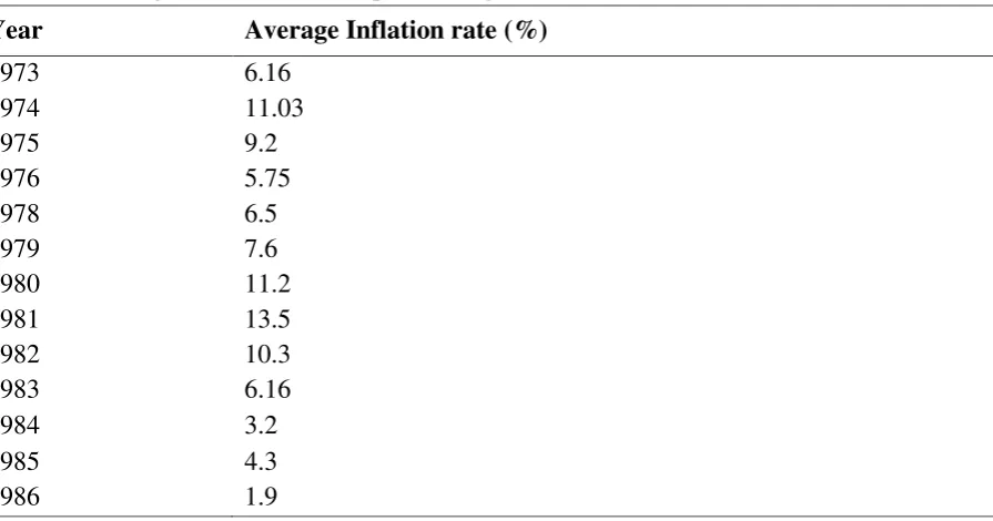
[image:17.595.78.526.403.638.2]The tight policy by the Fed during the 1920s and 1930s and the decline in MS figures in the United States in the course of contraction have brought the country to a severe recession and failed to stop inflation hikes until 1980s with the uprising of the Monetarism (Table 3). These figures prove the fallacy of Keynes believes about the ineffective rule of money and proving Friedman‘s view that MS do have an effect on the economy (Nelson, 2007). Unlike Keynes who adopted the ―money doesn‘t matter‖ slogan. Friedman and Schwartz, (1960) argued that managing MS -not the money demand- is what matters in fighting inflation. They explained their rationalization by a simple fact that people chose to hold money to suit their needs and when MS increases people would have more money in their pocket that exceeds their needs. Consequently, this surplus will be spent, pulling up aggregate demand, and the entire economy from a recession.
Table 3: Average inflation rate computed using CPI (1973-1986), U.S.
Source: Bureau of labor statistics
Friedman, (1968) has also developed a theory of MS targeting called ―K-percent rule‖. He proposed that MS should increase by a constant rate every year to meet the cyclical domestic demand for money. He then attributed inflationary pressures to any fluctuations in the MS expansion rate. The Federal Reserve began a "monetarist experiment" in October 1979, when the chairman Paul Volcker adopted an operating procedure based on the management of non-borrowed reserves. This procedure aimed to control the growth of M1 and M2 and hence to
Year Average Inflation rate (%)
1973 6.16
1974 11.03
1975 9.2
1976 5.75
1978 6.5
1979 7.6
1980 11.2
1981 13.5
1982 10.3
1983 6.16
1984 3.2
1985 4.3
reduce the double-digit inflation rates. As shown in Table 3, the disinflation effort was successful and leached the low-inflation regime that the United States has enjoyed since then. However, after 1982 the FED discontinued the MS targeting and it would be fair to say that since this time, the monetary and credit targeting have not played a central role in the U.S monetary policy, because of the unstable relationship between monetary aggregates and other macroeconomic variables Bernanke, (2006). Even Milton Friedman acknowledged that money supply targeting was less successful than he had hoped, in an interview with the Financial Times (London, 2003).
B. Monetary policy limitations
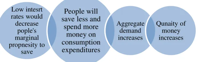
Friedman, (1968) stated that the ability of the monetary authority to peg MS changes to interest rates and unemployment is limited. First, the negative relation between interest rates and MS has illustrated the following figures. He differentiated between the perspective of the monetary authority and people liquidity preferences when explaining this hypothetical relation.
[image:18.595.71.520.357.513.2]Figure 1: The negative relation between interest rate and MS according to monetary authority point of view
Figure 2: The negative relation between interest rate and MS according to people‘s liquidity preference FED would like to increase MS FED purchases securities. As a result securities' prices increase
The raise in securities' prices will dimnish its yield The purachse action will raise bank funds
The whole qunatity of money in the
economy increases Low intesrt rates would decrease pople's marginal propnesity to save People will save less and
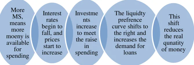
[image:18.595.141.458.582.682.2]Figure 3: The temporary relation between interest rate and MS
The former illustrations not only explain why monetary policy cannot peg interest rate except for a limited time but also clarify why the interest rate is a miss-leading indicator for the tightness or easiness of the monetary policy. Hence, Friedman advice policy makers to consider the rate of change in the quantity of money (M2) instead of interest rates (Friedman, 1968).
The core of the second limitation between monetary policy and unemployment lies in fluctuations around the natural rate of unemployment. When unemployment is at its natural rate, any further reductions means there is an excess demand for labor that creates an upward pressure on wages, and contrarily any increase imply that there is a shortage of demand for labor and thus creates a downward pressure on wages. The relationship between unemployment and wage level is manifested by the ‗Phillips curve‘, yet this curve has the major shortcoming that it does not consider the difference between nominal and real wages (Friedman, 1968). The following conjectural example elaborates further this limitation
i. Assume that people anticipate a high inflation rate of 75% a year.
ii. Real wages tend to increase with the anticipated inflation rate and supply of labor will increase.
iii. Nominal wages start to increase but still below inflation rates.
iv. A deflationary monetary policy will be engaged to bring prices down.
v. Nominal wage rises will last longer and will not respond quickly to the deflationary policy, which increases the unemployment rate in the economy above the natural rate of unemployment.
vi. The economy targets an unemployment level below the natural rate of unemployment.
vii. An expansionary monetary policy will be used to increase MS in the economy that will be translated into higher aggregate demand.
viii. Interest rate began to fall in order to stimulate investment and spending. Output, employment and people income rise but prices have not started to increase yet. ix. Producers respond to the increasingly demand by hiring more workers and engage
in further productions plans. Unemployment decreases and workers accept the existing nominal wages.
x. Inflation starts in consumer products before production inputs. Real wages start to decline because of inflation; workers start to demand higher nominal wages.
More MS, means more moeny is available for spending Interest rates begin to fall, and prices start to increase Investme nts increase to meet the raise in spending The liquidty prefrence curve shifts to
xi. Before inflation, unemployment falls below natural rates. However, after demanding higher nominal wages, real wages tend to rise towards the initial level, unemployment also increases with the endurable increase in MS and real wages. xii. For monetary authority to keep unemployment at its natural rate, it should
maintain inflation and MS growth. So we conclude that the tradeoff between inflation and unemployment comes from unanticipated inflation shocks and that inflation hikes may decrease unemployment.
C. The quantity theory of money:
Friedman, (1987) introduced the famous ―equation of exchange‖ or the ―quantity theory of
money‖ which describes the correlation between MS and the value of monetary transactions. It is an extension of Humes‘ ―price species flow theory‖ that was explained earlier. The classic's version of the quantity theory postulates that the price level reacts proportionally to changes to the stock of money. It can be derived from the following equation:
P = ƒ (M) (2) Assuming an exogenous potential output and full employment, in the short term, Yr can be
treated as a constant. Assuming further that the income velocity of money VY is exogenous and constant, equation 2 can be specified as P = AM, where A is the proportionality constant. Under these assumptions, money is neutral meaning that real output is completely independent of the stock or changes to the stock of money, hence money affects only the price level (Micheal, 2008).
D. Fisher’s quantity theory of money:
Fisher (1911) introduced his own version of the "equation of exchange" as follows:
(3)
Where M is the money supply, V is velocity, P is the price level and Y denotes the real output level. The right side of the equation PY is, therefore, nominal income or nominal output. We can rewrite equation 3 as M/P = V/Y, which states that real money supply (M/P), is equal to real money demand (V/Y). The following series of assumptions are then imposed: first, M is assumed to be exogenous and thus subject to the full control of the monetary authority. Second, V is constant, third, the aggregate nominal demand component cause changes in nominal income, i.e. causality runs from MV to PY. Fourth, movements in nominal output
PY are driven by movements in M. and finally, Y is constant at the full employment level. So MS raises feeds entirely into higher price levels.
E- Cambridge approach:
version focused on money demand instead of the money supply. He argued that a certain portion of the money supply will not be used for transactions; instead, it will be held for the security of having cash on hand. This portion of nominal income PY cash is commonly represented as k as shown in Equation 4
=k.PY (4)
Assuming that the economy is at equilibrium (Md = M), Y is exogenous, and k is fixed in the short run, the Cambridge equation is equivalent to the equation of exchange with velocity equal to the inverse of k:
M.1/ k=PY
The Cambridge equation led to Keynes‘s attack on the quantity theory and the Monetarist revival of the theory (Froyen, 1990).
E- Monetarist liquidity preference theory:
Friedmans‘ theory addressed the main weaknesses of the classical quantity theory, mainly ignoring the velocity of money and its determinants. Let us take a look at the updated
monetarists‘ version of the ―equation of exchange‖ after adding new variables. Friedman, (1956) expressed the money demand (Md) function as follows
〈 〉 (5)
i. Inflation rate: denoted by P, where a high price level implies a low 'price of money' so
that ƒ'P> 0.
ii. The prices of substitutive goods: here interpreted as the real return of other financial claims, such as yields on fixed-interest bonds Rb, and yield from holding real assets Re, where ƒ'Rb< 0 and ƒ'Re< 0 . The yield from holding real assets rather than financial claims corresponds to the rate of inflation so that ƒ'(1/P)(dP/dt) < 0.
iii. The budget constraint: here is expressed by the permanent income Y, where ƒ'Y> 09. iv. The liquidity of total assets: here Friedman defines W, as the ratio of non-human
assets to human capital. As human capital is less liquid as non-human assets, it
follows that ƒ'w< 0.
v. Preferences: here Friedman uses the term U to account for preference changes. Yet remains vague. It is more like a ‗catch-all‘ term to make sure that this equation account for all possible variables.
Monetarism assumes the people are free from money illusion, the nominal money demand Md is linearly homogeneous in nominal variables (here: P and Y), so that,
9
〈 〉 (6) 〈 〉 (7)
Solving Equation 7 for Y and using the equilibrium condition Md = MS, we get
[ 〈 〉 ] (8)
With a stable money demand function and the exogenous nature of MS (predetermined by the monetary authority), nominal output Y can be directly controlled. Hence, from the monetarist point of view, the money supply is, or should be, the central variable of economic policy (Micheal, 2008)
In summary,
Monetarists did not embrace the classical ―laissez-faire‖ rule, rather they recommend controlling the money supply growth rate as a remedy for long and short run market distortions. They also asserted that nominal aggregate demand is affected by aggregate supply, therefore –unlike the Keynesians- emphasized the healing role of monetary policy in fiscal policy. Another departure from the Keynesians is the assumption of non- rigid of prices and wages. The quantity theory of money asserts the direct relationship between MS and price level.According to Friedman‘s (1960) view of the monetary transmission mechanism, the increase in MS, will shift LM curve to the right, bringing down the interest rate and raising nominal output. However, the impact on the real output is limited due to the money velocity reduction. The former process constructs the biggest difference between the Keynesians and the monetarists. The monetarists argue that a complete effect on output will be realized, while the Keynesians argue that velocity absorbs a good part of the impact and thus the final effect on nominal output will be smaller.
During the 1980s the correlation between the excess supply of money and inflation had apparently collapsed. This eventually caused central banks in different countries to place less importance on the money supply as a target of monetary policy. Instead, they switched to having exchange rate targets, and lately to inflation targets as a monetary anchor (Micheal, 2008).
1-2-6. Neo classical-Keynesian synthesis
A. A necessary introduction
Klein, (1946) was one of the first economists to use the term ―macroeconomics‖, in his paper he stated that ―Many of the newly constructed mathematical models of economic systems, especially business-cycle theories, are very loosely related to the behavior of individual households or firms which must form the basis of all theories of economic behavior ―. How to reconcile the two visions of the economy was the main concern during this era. The microeconomic side based on Adam Smith‘s invisible hand and Alfred Marshall‘s supply and demand curves. And the macroeconomic side mainly founded on Keynes analysis of the aggregate economy. Early Keynesians, such as Samuelson and Tobin, thought they had
reconciled these visions in what is sometimes called the ―neo classical-Keynesian synthesis.‖ Although this synthesis is coherent, it is also vague and incomplete. These shortcomings forced the neo-classical and neo-Keynesians to reject this methodology and develop a new approach (Manikw, 2006).
B. Neo- Keynesians main assumptions
This school of thought is developed partly as a response to the criticisms of the Keynesians macroeconomics by the neo-classical macroeconomics adherents. These critics revolve around the assumptions of several market failures and the price stickiness10. Still, neo-Keynesians agree with neo-classical about the neutrality of MS in the long run, but because of the price stickiness assumption, neo-Keynesians believe that MS fluctuations in the short run directly influence output and employment levels. However, they don‘t advocate the use of expansive monetary for short run gains in output and employment because inflationary pressures that will occur will be hardly removed unless the economy was subject to a recession or an external shock (e.g. fall in consumer confidence) (Olivier and Jordi, 2007). Studies of the optimal monetary policy in the neo-Keynesians‘ Dynamic Stochastic General Equilibrium (DSGE) models emphasized the use of nominal interest rate adjustments in adjusting inflation and output gaps. Eventually, stabilizing inflation will stabilize both output and employment, or what is known as the called this ―Divine coincidence‖ (Blanchard and Gali, 2007).
C. Inflation
Lerner (1983) was the first Keynesian economist to stress the possibility and importance of inflation in the Keynesian models. In his theory the ―functional finance‖, he stressed on the governmental role of controlling inflation and deflation and considered this as the primary
10
objective of the government policy. He later incorporated the unemployment-inflation
[image:24.595.77.311.205.375.2]tradeoff explained by ―Phillips curve‖ and the possibility of stag inflation later before the emergence of neo-Keynesians. Samuelson and Solow, (1960) were the first to integrate the "Phillips Curve" into the Neo-Keynesian edifice. Keynes, (1940) have introduced the concept of the demand-pull inflation, which reasons inflationary waves to excess demand, that will bring about higher levels of supply and output by the multiplier effect until the economy reaches full employment. At this level, output stagnates and with higher aggregate demand levels, raising goods price will be the only way to clear the markets.
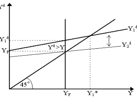
Figure 4: Demand-pull inflation (inflationary gap).
The demand pulls inflation is elaborated by the 45 income-expenditure diagram in Figure 4, where YF is full employment output and Y1d is aggregate demand. Note that the market-clearing level of output is Y1*, but it is not achievable – thus the ―inflationary gap" is the difference between YF and Y1*. Keynes's, (1940) argument can be restated as follows: as money wages lag behind prices in adjustment, the rise in prices will, therefore, lead to a distribution of income away from wage-earners and towards profit-earners. He posited that, as workers have greater marginal propensities to consume than profit-earners, the redistribution of income induced by the inflationary gap will thereby lead to lower aggregate demand and thus close the gap, i.e. the aggregate demand curve flattens and falls in Figure 4 from Y1d to Y2d .
The problem persists as workers demand higher wages. The time lag for nominal wages to adjust depends upon the barraging power of their labor union and the flexibility of labor laws in their country. Once nominal wages increase, income redistributes away from profit-earners and towards wage-earners so that demand rises again (from Y2d to Y1d) and thus the inflationary gap re-emerges. But that inflationary gap, as noted earlier, leads to another price rise, redistribution of income to profiteers, etc. Thus, the whole process repeats itself continuously so that there will be, effectively, sustained, continual increases in prices.
(9)
Where P is price, m is markup profit and w is wages. Hence with the economy approaching full employment, unemployment starts to fall and with labor demanding higher wages by the help of their labor unions bargaining power, Employers set higher prices while sustaining the markup profit. Soon labor finds that their wage increase is not real and thus demand higher wages, this process continues to create a sustained increase in the price level in the economy. Lerner, (1974) stressed that the blame doesn‘t all fall on the workers‘ shoulders alone, seeking higher profit by owners also could create similar inflation, even in the presence of high unemployment i.e. Stag inflation. Also, Lerner and Colander, (1980) introduced a new remedy for stagflation, known as the Markup-Anti-inflation Plan (MAP). They proposed that the right to change prices should be assigned to firms in the form of a fixed supply of tradable vouchers, so that if a firm attempts to raise its prices, it would have to cash in its vouchers and thus abandon its right to further price increases and a firm which lower prices would gain vouchers in return. If a particular firm wanted to raise prices further, then it would have to purchase vouchers from other firms on the open market. In their view, these added costs would make profit-induced price rises less appealing to firms and thus help bring stagflation under control.
[image:25.595.74.303.400.565.2]D. Phillips curve explained:
Figure 5: Phillips curve of a single industry.
that there is a definite inflation-unemployment trade-off that could be managed by policy-makers.11
E. Natural rate hypothesis “Milton Friedmans’missing equation”:
Milton Friedman couldn‘t decide what is the proper effect of MS increase, indeed it will raise
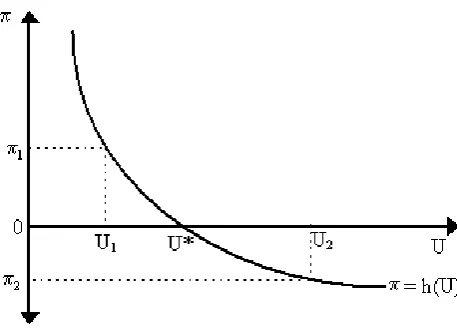
[image:26.595.76.371.310.535.2]aggregate nominal demand, but that could happen because of the rise in the price level or/and rise in output. This constitutes what is known as the ―missing equation‖. As Phillips curve provided the neo-Keynesians with an empirical rationale for setting their dynamic nominal wage which was absent in their system, it has also provided the monetarists with their own missing equation. The theory of the ―natural rate hypothesis‖ introduced by Friedman, (1968) compiled the missing parts. The original Phillips curve asserted that there is a negative relation between nominal wage inflation and unemployment rate. Figure (6) presents the transmission from wage into price inflation.
Figure 6: Natural rate hypothesis
Unemployment (U) estimated as the difference between labor supply and labor demand , in neo-classical theory, household supply labor at a particular wage level (w/p), at this wage level there is a particular amount of labor supplied (LS*). Labor demand is established by profit-maximizing firm conditions. The natural rate of unemployment at a particular wage level (U*) equals (Ls*- Ld)/Ls*. Assume that U* is the actual prevailing unemployment level. Phillips curve will pass through U* at zero inflation rate. Assume government is targeting unemployment level U1 which is below U *, by increasing nominal demand, firms will respond by increasing output and hiring more workers. To do so,
11
firms raise nominal wages to attract those workers out of leisure Gw>0 (at point a on the graph (U1, but with the assumption that there is no productivity growth, then the increase in nominal wages will be inflationary Workers realize that their real income has not changed, so they leave the market and unemployment jump back to U * however, at a higher inflation rate (at point b (U*,
F- Theory of adaptive expectations:
Friedman (1968) and Phelps (1967, 1968) proposed that agents have some kind of adaptive expectations of prices that are extrapolated from their experience of past inflation. Agents increase their supply only if current inflation levels are higher than expected levels > e. In other words, if they misperceive what actual inflation is and only if firms increase wages faster than expected inflation. Expectations-augmented Phillips curve in which can be expressed as follows:
(10)
Phillips curve is now related to inflation expectation, if e=0, then we revert to the original version of Phillips curve. However, if we have positive inflation expectation e>0, then each higher level of expectation corresponds to a higher short-run Phillips curve. In the long run, e
= , so expectations-augmented Phillips curve tends to be a vertical line at the natural rate of unemployment (Friedman, 1968). In other words, there is no stable long-run trade-off between inflation and unemployment.
G- The impact of unanticipated inflationary shocks:
According to the expectations-augmented Phillips curve, Abel and Bernanke, (1994) stated that unemployment will fall below the natural rate only when inflation is unanticipated. Neo-classical and neo- Keynesians diverge at this point. Classicals consider that policy (such as more rapid monetary expansion) that increase the growth rate of aggregate demand act primarily to raise actual and expected inflation together -because people are assumed to have rational expectations- which hinders the ability of the government to initiate unexpected shocks. Hence, any systematic attempt to affect unemployment will be thwarted by the rapid adjustment of inflation expectations and the government cannot keep actual inflation above expected inflation.
In line with the neo-classical, Friedman, (1968) argued that the only way of maintaining unemployment below the natural rate is that the government continuously accelerate the rate of nominal aggregate demand growth. The inflation rate, of course, would spiral upwards to a high degree of hyperinflation. At any point, the government relented in its acceleration, the unemployment rate would jump right back to the natural rate, leaving a very high inflation rate and the government's accelerating efforts would have been wasted.
H- Expectations-augmented Phillips curve
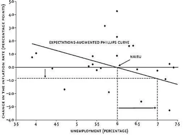
The theory of the Phillips curve seemed stable. Data from the 1960's modeled the trade-off between unemployment and inflation well. However, data from the 1970's and onward did not follow the trend of the classic Phillips curve. For many years, both the rate of inflation and the rate of unemployment were rising. These findings pushed many economists to accept a central tenet of the Philips curve theory, which asserts that there is a specific rate of unemployment that, if maintained, would be compatible with a stable rate of inflation. Many call this rate the ―No Accelerating Inflation Rate of Unemployment‖ (NAIRU).12
Figure 7 plots fluctuations in inflation against unemployment rate from 1976 to 2002. The expectations-augmented Phillips curve is the straight line that best fits the points on the graph (the regression line). It summarizes the inverse relationship. According to the regression line, NAIRU (i.e., the rate of unemployment for which the change in the rate of inflation is zero) is about 6 percent, while the slope of the Phillips curve indicates the speed of price adjustment. If the economy is at NAIRU with an inflation rate of 3 percent and the government would like to reduce the inflation rate to zero. Figure 7 suggests that contractionary monetary and fiscal policies that drove the average rate of unemployment up to about 7 percent (i.e., one point above NAIRU) would be associated with a reduction in inflation of about one percentage point per year. Thus, if the government‘s policies caused the unemployment rate to stay at about 7 percent, the 3 percent inflation rate would, on average, be reduced one point each year falling to zero in about three years (Kevin, 2007).
12
Figure 7: Expectations-augmented Phillips curve and NAIRU‖. # Notes: Inflation is based on the Consumer Price Index.
Source: Bureau of labor statistics.
This theory created a controversy between a wide range of scientists about the existence of this NAIRU and the presence of the natural rate of unemployment. Some Neo-Keynesian and some free-market economists hold that there is only a weak tendency for an economy to return to NAIRU. They argue that there is no natural rate of unemployment to which the actual rate tends to return. Instead, when actual unemployment rises and remains high for some time, NAIRU also rises. The dependence of NAIRU on actual unemployment is known
as the ―hysteresis hypothesis‖. The hysteresis hypothesis appears to be more relevant to Europe, where unionization is higher and where labor laws create numerous barriers to hiring and firing than it is to the U.S (Kevin, 2007).
I. Neo-classical theory of Rational expectations “surprise money only matters”:
Lucas, (1973) and Sargent, (1973) postulated that a systematic monetary policy has no effect on output. Only policy shocks can influence output. Contrary to Friedman's "only money matters", the neo-Classical' raise the watchword of ―only surprise money matters". Sargent,
(1973) introduced a new theory that replaces Friedman‘s adaptive expectations with what they call ―theory of rational expectations‖. This theory shows that not only there is no long -run trade-off between inflation and unemployment, but that there is not even a short--run trade-off. The neo-classical‘ objection was that Friedman's "adaptive expectations" assume that agents are making a systematic error of inferring future inflation rates based on current ones. On contrary, the rational expectations hypothesis argues that agents make full use of their information and do not make a persistent systematic error.
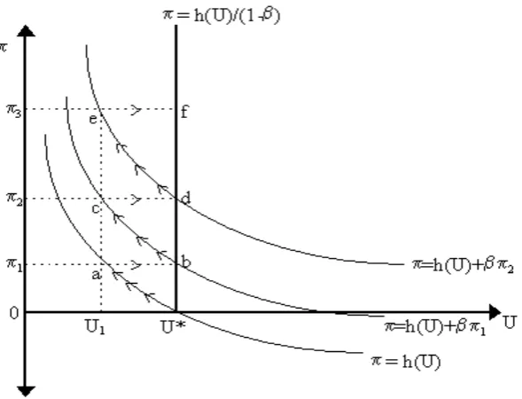
moved up the short-run Phillips Curve from the initial position (U = U*, π = 0) to point a (U = U1, π = π1) but rather would have jumped straight to point b (U = U*, π = π1) on the long-run Phillips curve. In other words, the government would have been unable to lower unemployment to U1 even temporarily.
This does not mean that unemployment cannot fall below U* as a response to monetary acceleration. But this acceleration would have to happen unsystematically or randomly so that agents would not be able to form expectations. In this case, then inflation expectations could not be properly constructed and agents would indeed move up to point a (U = U1, π =
π1). But this is temporary: as soon as they realize what happened -similar to the Monetarist‘s scenario- they would leave the labor market again and unemployment reverts back to U*.
In summary,
this section explained the nature of the term ―synthesis‖ that combines both the classical and the Keynesian theories. This blended theory was developed by Hicks, (1937). Although this synthesis basically has quite many issues that are related to different aspects of macroeconomics and microeconomics, our discussion was mainly revolving around the theme of our book, monetary policy.The neo-classical‘ main contribution to this synthesis, is their theory of rational expectations that contradicts with the idea of Phillips curve. It states that there is no tradeoff between inflation and unemployment neither in short run nor long run, unless the government was able to make aggregate demand accelerating shocks that agents would not expect. These shocks, in turn, could create a temporary trade-off in short time but only temporary, as when agents realize the government plan then this trade off will be exploited. Neo-Keynesians agree with the neo-classical about the nonexistence of this trade-off in long run, however, they defend its presence in short run. Using their theory of adaptive expectations that current inflation expectations are created from past inflation experience. On the other side, they raise doubts about the ability of the government to push down unemployment level below what is called the natural rate of unemployment, because of the money illusion- which tempted workers to leave leisure and get to work- soon will vanish and they will find that their real wages have not improved because of the higher price levels. Therefore, unemployment gets reverts back to the ―natural rate of unemployment‖ forming the neo-Keynesians‘ version of Philips curve known as the expectations-augmented Phillips curve. This money illusion can endure and reduce unemployment, only when the government continuously increases aggregate demand, but this is a dangerous remedy because once the government for any reason stops this process, the economy will suffer from a hyperinflation. A group of opponents introduced the hysteresis hypothesis, which conditionals the existence of the natural rate of unemployment –as well the applicability of the expectations-augmented Philips curve- to labor laws and rigidity of hiring and firing rules in the country.
every mean higher inflation. By the time the government reaches its full employment and become forced to stop the process of monetary expansion otherwise it will go bankruptcy or the money will lose its value as a medium of exchange. Eventually, it will stop the accelerating process and higher price levels will remain.
1-2-7. New-Neo classical synthesis
Our time-travel journey has finally come to an end. The new neo-classical synthesis (NNS) represents the current models which govern monetary policy actions today and the baseline of the coming chapters. They are complex since they involve intertemporal optimization, rational expectations, and monopolistic competition. Along with applications on inflation targeting wherein the rate of inflation (positive or near zero) is targeted by the monetary authority. The NNS sets four central monetary policy guidelines. First, their models suggest that the impact of the monetary policy on real economic activities is resilient, due to the slow adjustment of individual prices and the general price level. Second, even in settings with costly price adjustments, they suggest a low scaled long-run trade-off between inflation and output at the low inflation rate. Third, NNS models suggest significant gains from eliminating inflation, which stems from increased transactions efficiency and reduced relative price distortions, and finally, they assert that credibility plays an important role in realizing monetary policy actions (Goodfriend and King, 1997).
NNS models stress that economic fluctuations cannot be interpreted or understood independent of monetary policy. From a normative perspective, the NNS suggest that aggregate demand must be managed by the monetary policy in order to deliver efficient macroeconomic outcomes. The NNS defines two mechanisms for transmitting the monetary policy actions to the real economy. The First channel is through its influence on the goods‘ prices and the marginal cost of production (average markup), as monetary policies can raise aggregate demand and lowers the average markup that in turn create surges in output and employment. The second is attributed to the impact of MS fluctuations on aggregate demand, which trigger changes in aggregate supply (Goodfriend and King, 1997).
1-3. Connecting the dots:
Following Mabrouk and Hassans‘, (2012) tabulated summary of monetary developments in the history of macroeconomics. The section presents the main highlights from the previous sections while underlying the main theme or contribution of each school regarding monetary policy actions and its impact on the economy.
1- The first form that describes the correlation between MS (gold or silver) and inflation were first introduced by David Hume with the name price species flow, then this theory was
by the monetarists‘ theory of liquidity preference with more control variables like a budget constraint, preference, the price of related goods.
2- Classical and Austrians put a great emphasize on the laissez-faire rule of non-government intervention.
3- The market rigidness assumption was first used by the classical economist David
Ricardo in his theory ―beneficial inflation ―which describe the gap between MS expansion
and inflation, that could be used as a remedy for unemployment. Later the same concept was used by Keynes in his theory that viewed monetary policy as a remedy for unemployment that could push the economy towards full employment before indexed to inflation.
4- According to the Keynesians, fiscal policies are more influential than monetary policies because the economy might enter a liquidity trap that blocks monetary changes from affecting the economy.
5- Free banking –according to the Austrians- and natural adjustment of interest rates are their suggested policies to prevent market distortion problems like inflation and recession.
6- Keynesians agreed with the Monetarists about the need for government intervention to clear the market distortions and solve problems like inflation and unemployment, but they disagreed on which policy action is required. Keynesians view inflation as a demand-side problem that is managed by fiscal policies, and monetarists considered inflation as a supply side problem that is controlled by the monetary authority.
7- Friedman‘s K-percent rule was suggested by the Monetarists as a cure for high inflation and a catalyst for economic growth, through both reducing unemployment and increasing nominal aggregate demand.
8- Monetarists postulated that the negative correlation between MS and interest rate exist for a limited period. After some time, interest rate gets back to its initial position, or even higher because of people expectations.
9- Classical agreed with monetarists about the possibility of bringing down unemployment rate below the natural rate of unemployment via unanticipated inflation shocks.
11- Neo-Keynesians believe in the short-run tradeoff between inflation and unemployment and its absence in the long run, while the neo-classical rejected the existence of this swap neither in the short nor in the long run.
Chapter two: the theory of optimal monetary policy
2-1. Monetary Transmission Mechanisms (MTMs)
Monetary policy is an effective and a powerful tool, but sometimes it has unexpected consequences. To conduct a successful monetary policy, the monetary authority should have an accurate assessment of the timing and the effect of their policies on the economy. MTMs describe how policy changes in nominal money stock or short-term interest rate affect real economic variables such as employment and aggregate output (Ireland, 2004).
2-1-1. Interest rate channel:
We start our analysis with the interest rate channel. This channel plays an important role in transmitting monetary changes to households and firms (Al Mashat and Billmeier, 2007). The traditional Keynesian interest rate channel in the IS-LM model can be disentangled into two steps: a- the transmission from short-term nominal interest rate to the long-term real interest rate. b- The impact of real interest rate developments on aggregate demand and production (Fabrizo et al., 2006). The following example clarifies how this channel works, suppose that the authority decided to conduct a tight monetary policy. This, in turn, raises short and long run nominal interest rate13. This appreciation leads to a decline in business and residual investments by households, which causes a decline in aggregate output. Changes in interest rates entail two conflicting effects, an income effect that is attributed to the income of the interest bearing asset holders. And the second is a substitution effect, which pushes people towards savings accumulation instead of consumption (Fabrizo et al., 2006).
2-1-2. Exchange rate channel:
There are two main methods of altering exchange rate of local currencies, the first is interest rate fluctuations, for instance when real interest rate rises, domestic currency deposits become more attractive compared with foreign currency deposits that lead to appreciation in the local
13