Bayesian Learning of Non-compositional Phrases with Synchronous Parsing
Hao Zhang
Computer Science Department University of Rochester
Rochester, NY 14627
Chris Quirk Microsoft Research One Microsoft Way Redmond, WA 98052 USA [email protected]
Robert C. Moore Microsoft Research One Microsoft Way Redmond, WA 98052 USA [email protected]
Daniel Gildea
Computer Science Department University of Rochester
Rochester, NY 14627 [email protected]
Abstract
We combine the strengths of Bayesian mod-eling and synchronous grammar in unsu-pervised learning of basic translation phrase pairs. The structured space of a synchronous grammar is a natural fit for phrase pair proba-bility estimation, though the search space can be prohibitively large. Therefore we explore efficient algorithms for pruning this space that lead to empirically effective results. Incorpo-rating a sparse prior using Variational Bayes, biases the models toward generalizable, parsi-monious parameter sets, leading to significant improvements in word alignment. This prerence for sparse solutions together with ef-fective pruning methods forms a phrase align-ment regimen that produces better end-to-end translations than standard word alignment ap-proaches.
1 Introduction
Most state-of-the-art statistical machine transla-tion systems are based on large phrase tables ex-tracted from parallel text using word-level align-ments. These word-level alignments are most of-ten obtained using Expectation Maximization on the conditional generative models of Brown et al. (1993) and Vogel et al. (1996). As these word-level align-ment models restrict the word alignalign-ment complex-ity by requiring each target word to align to zero or one source words, results are improved by align-ing both source-to-target as well as target-to-source,
then heuristically combining these alignments. Fi-nally, the set of phrases consistent with the word alignments are extracted from every sentence pair; these form the basis of the decoding process. While this approach has been very successful, poor word-level alignments are nonetheless a common source of error in machine translation systems.
A natural solution to several of these issues is unite the word-level and phrase-level models into one learning procedure. Ideally, such a procedure would remedy the deficiencies of word-level align-ment models, including the strong restrictions on the form of the alignment, and the strong inde-pendence assumption between words. Furthermore it would obviate the need for heuristic combina-tion of word alignments. A unified procedure may also improve the identification of non-compositional phrasal translations, and the attachment decisions for unaligned words.
In this direction, Expectation Maximization at the phrase level was proposed by Marcu and Wong (2002), who, however, experienced two major dif-ficulties: computational complexity and controlling overfitting. Computational complexity arises from the exponentially large number of decompositions of a sentence pair into phrase pairs; overfitting is a problem because as EM attempts to maximize the likelihood of its training data, it prefers to directly explain a sentence pair with a single phrase pair.
In this paper, we attempt to address these two is-sues in order to apply EM above the word level.
We attack computational complexity by adopting the polynomial-time Inversion Transduction Gram-mar framework, and by only learning small non-compositional phrases. We address the tendency of EM to overfit by using Bayesian methods, where sparse priors assign greater mass to parameter vec-tors with fewer non-zero values therefore favoring shorter, more frequent phrases. We test our model by extracting longer phrases from our model’s align-ments using traditional phrase extraction, and find that a phrase table based on our system improves MT results over a phrase table extracted from traditional word-level alignments.
2 Phrasal Inversion Transduction Grammar
We use a phrasal extension of Inversion Transduc-tion Grammar (Wu, 1997) as the generative frame-work. Our ITG has two nonterminals: X and
C, where X represents compositional phrase pairs that can have recursive structures andC is the pre-terminal over pre-terminal phrase pairs. There are three rules withXon the left-hand side:
X → [X X], X → hX Xi, X → C.
The first two rules are the straight rule and in-verted rule respectively. They split the left-hand side constituent which represents a phrase pair into two smaller phrase pairs on the right-hand side and order them according to one of the two possible permuta-tions. The rewriting process continues until the third rule is invoked. C is our unique pre-terminal for generating terminal multi-word pairs:
C → e/f.
We parameterize our probabilistic model in the manner of a PCFG: we associate a multinomial dis-tribution with each nonterminal, where each out-come in this distribution corresponds to an expan-sion of that nonterminal. Specifically, we place one multinomial distribution θX over the three expan-sions of the nonterminalX, and another multinomial distributionθC over the expansions ofC. Thus, the parameters in our model can be listed as
θX= (Phi, P[], PC),
wherePhiis for the inverted rule,P[]for the straight rule,PCfor the third rule, satisfyingPhi+P[]+PC =
1, and
θC= (P(e/f), P(e′/f′), . . .),
wherePe/fP(e/f) = 1is a multinomial distribu-tion over phrase pairs.
This is our model in a nutshell. We can train this model using a two-dimensional extension of the inside-outside algorithm on bilingual data, assuming every phrase pair that can appear as a leaf in a parse tree of the grammar a valid candidate. However, it is easy to show that the maximum likelihood training will lead to the saturated solution wherePC = 1— each sentence pair is generated by a single phrase spanning the whole sentence. From the computa-tional point of view, the full EM algorithm runs in
O(n6)wherenis the average length of the two in-put sentences, which is too slow in practice.
The key is to control the number of parameters, and therefore the size of the set of candidate phrases. We deal with this problem in two directions. First we change the objective function by incorporating a prior over the phrasal parameters. This has the effect of preferring parameter vectors in θC with fewer non-zero values. Our second approach was to constrain the search space using simpler align-ment models, which has the further benefit of signif-icantly speeding up training. First we train a lower level word alignment model, then we place hard con-straints on the phrasal alignment space using confi-dent word links from this simpler model. Combining the two approaches, we have a staged training pro-cedure going from the simplest unconstrained word based model to a constrained Bayesian word-level ITG model, and finally proceeding to a constrained Bayesian phrasal model.
3 Variational Bayes for ITG
alignment models is the EM algorithm (Brown et al., 1993) which iteratively updates parameters to maximize the likelihood of the data. The drawback of maximum likelihood is obvious for phrase-based models. If we do not put any constraint on the dis-tribution of phrases, EM overfits the data by mem-orizing every sentence pair. A sparse prior over a multinomial distribution such as the distribution of phrase pairs may bias the estimator toward skewed distributions that generalize better. In the context of phrasal models, this means learning the more repre-sentative phrases in the space of all possible phrases. The Dirichlet distribution, which is parameter-ized by a vector of real values often interpreted as pseudo-counts, is a natural choice for the prior, for two main reasons. First, the Dirichlet is conjugate to the multinomial distribution, meaning that if we select a Dirichlet prior and a multinomial likelihood function, the posterior distribution will again be a Dirichlet. This makes parameter estimation quite simple. Second, Dirichlet distributions with small, non-zero parameters place more probability mass on multinomials on the edges or faces of the probabil-ity simplex, distributions with fewer non-zero pa-rameters. Starting from the model from Section 2, we propose the following Bayesian extension, where
A ∼ Dir(B) means the random variableA is dis-tributed according to a Dirichlet with parameterB:
θX |αX ∼Dir(αX),
θC|αC ∼Dir(αC),
[X X]
hX Xi C
X ∼Multi(θX),
e/f |C ∼Multi(θC).
The parametersαX andαC control the sparsity of the two distributions in our model. One is the distri-bution of the three possible branching choices. The other is the distribution of the phrase pairs. αC is crucial, since the multinomial it is controlling has a high dimension. By adjusting αC to a very small number, we hope to place more posterior mass on parsimonious solutions with fewer but more confi-dent and general phrase pairs.
Having defined the Bayesian model, it remains to decide the inference procedure. We chose Vari-ational Bayes, for its procedural similarity to EM and ease of implementation. Another potential op-tion would be Gibbs sampling (or some other sam-pling technique). However, in experiments in un-supervised POS tag learning using HMM structured models, Johnson (2007) shows that VB is more ef-fective than Gibbs sampling in approaching distribu-tions that agree with the Zipf’s law, which is promi-nent in natural languages.
Kurihara and Sato (2006) describe VB for PCFGs, showing the only need is to change the M step of the EM algorithm. As in the case of maximum like-lihood estimation, Bayesian estimation for ITGs is very similar to PCFGs, which follows due to the strong isomorphism between the two models. Spe-cific to our ITG case, the M step becomes:
˜
P[](l+1)= exp(ψ(E(X→[X X]) +αX)) exp(ψ(E(X) +sαX))
,
˜
Phi(l+1)= exp(ψ(E(X→ hX Xi) +αX)) exp(ψ(E(X) +sαX))
,
˜
PC(l+1)= exp(ψ(E(X→C) +αX)) exp(ψ(E(X) +sαX))
,
˜
P(l+1)(e/f) = exp(ψ(E(e/f) +αC))
exp(ψ(E(C) +mαC))
,
whereψis the digamma function (Beal, 2003),s= 3is the number of right-hand-sides forX, andmis the number of observed phrase pairs in the data. The sole difference between EM and VB with a sparse prior α is that the raw fractional counts c are re-placed byexp(ψ(c+α)), an operation that resem-bles smoothing. As pointed out by Johnson (2007), in effect this expression adds toca small value that asymptotically approachesα−0.5ascapproaches
∞, and 0 as c approaches0. For small values of
α the net effect is the opposite of typical smooth-ing, since it tends to redistribute probably mass away from unlikely events onto more likely ones.
4 Bitext Pruning Strategy
smaller than the possible scriptO(n4), where nis the average sentence length. Pruning the span pairs (bitext cells) that can participate in a tree (either as terminals or non-terminals) serves to not only speed up ITG parsing, but also to provide a kind of ini-tialization hint to the training procedures, encourag-ing it to focus on promisencourag-ing regions of the alignment space.
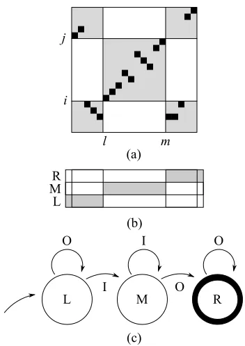
Given a bitext cell defined by the four boundary indices(i, j, l, m)as shown in Figure 1a, we prune based on a figure of meritV(i, j, l, m) approximat-ing the utility of that cell in a full ITG parse. The figure of merit considers the Model 1 scores of not only the words inside a given cell, but also all the words not included in the source and target spans, as in Moore (2003) and Vogel (2005). Like Zhang and Gildea (2005), it is used to prune bitext cells rather than score phrases. The total score is the product of the Model 1 probabilities for each column; “inside” columns in the range[l, m]are scored according to the sum (or maximum) of Model 1 probabilities for
[i, j], and “outside” columns use the sum (or maxi-mum) of all probabilities not in the range[i, j].
Our pruning differs from Zhang and Gildea (2005) in two major ways. First, we perform prun-ing usprun-ing both directions of the IBM Model 1 scores; instead of a single figure of meritV, we have two:
VF and VB. Only those spans that pass the prun-ing threshold in both directions are kept. Second, we allow whole spans to be pruned. The figure of merit for a span isVF(i, j) = maxl,mVF(i, j, l, m). Only spans that are within some threshold of the un-restricted Model 1 scoresVF andVBare kept:
VF(i, j)
VF
≥τs and
VB(l, m)
VB
≥τs.
Amongst those spans retained by this first threshold, we keep only those bitext cells satisfying both
VF(i, j, l, m)
VF(i, j)
≥τb and
VB(i, j, l, m)
VB(l, m)
≥τb.
4.1 Fast Tic-tac-toe Pruning
The tic-tac-toe pruning algorithm (Zhang and Gildea, 2005) uses dynamic programming to com-pute the product of inside and outside scores for all cells inO(n4) time. However, even this can be slow for large values ofn. Therefore we describe an
Figure 1: (a) shows the original tic-tac-toe score for a bitext cell (i, j, l, m). (b) demonstrates the finite state representation using the machine in (c), assuming a fixed source span(i, j).
improved algorithm with best casen3performance. Although the worst case performance is alsoO(n4), in practice it is significantly faster.
To begin, let us restrict our attention to the for-ward direction for a fixed source span(i, j). Prun-ing bitext spans and cells requiresVF(i, j), the score of the best bitext cell within a given span, as well as all cells within a given threshold of that best score. For a fixed iandj, we need to search over the starting and ending points l and m of the in-side region. Note that there is an isomorphism be-tween the set of spans and a simple finite state ma-chine: any span (l, m) can be represented by a se-quence oflOUTSIDEcolumns, followed bym−l+1
INSIDE columns, followed by n − m + 1 OUT-SIDE columns. This simple machine has the re-stricted form described in Figure 1c: it has three states, L, M, and R; each transition generates ei-ther an OUTSIDE column O or an INSIDE column
[image:4.612.330.506.56.305.2]O(0) =O(n+ 1) = 1andI(0) =I(n+ 1) = 0. Directly computing O and I would take time
O(n2) for each source span, leading to an overall runtime ofO(n4). Luckily there are faster ways to find the inside and outside scores. First we can pre-compute following arrays inO(n2)time and space:
pre[0, l] := P(tl|NULL)
pre[i, l] := pre[i−1, l] +P(tl|si) suf[n+ 1, l] := 0
suf[i, l] := suf[i+ 1, l] +P(tl|si)
Then for any (i, j), O(a) = P(ta|NULL) +
P
b6∈[i,j]P(ta|sb) = pre[i−1, a] +suf[j + 1, a].
I(a) can be incrementally updated as the source span varies: when i = j, I(a) = P(ta|NULL) +
P(ta|si). Asj is incremented, we add P(ta|sj)to
I(a). Thus we have linear time updates forOandI. We can then find the best scoring sequence using the familiar Viterbi algorithm. Letδ[a, σ]be the cost of the best scoring sequence ending at in stateσ at timea:
δ[0, σ] := 1ifσ=L;0otherwise
δ[a, L] := δ[a−1, L]·O(a)
δ[a, M] := max
σ∈L,M{δ[a−1, σ]} ·I(a)
δ[a, R] := max
σ∈M,R{δ[a−1, σ]} ·O(a)
Then VF(i, j) = δ[n + 1, R], using the isomor-phism between state sequences and spans. This lin-ear time algorithm allows us to compute span prun-ing in O(n3) time. The same algorithm may be performed using the backward figure of merit after transposing rows and columns.
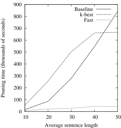
Having cast the problem in terms of finite state au-tomata, we can use finite state algorithms for prun-ing. For instance, fixing a source span we can enu-merate the target spans in decreasing order by score (Soong and Huang, 1991), stopping once we en-counter the first span below threshold. In practice the overhead of maintaining the priority queue out-weighs any benefit, as seen in Figure 2.
An alternate approach that avoids this overhead is to enumerate spans by position. Note thatδ[m, R]· Qn
a=m+1O(a) is within threshold iff there is a span with right boundary m′ < m within thresh-old. Furthermore if δ[m, M] · Qna=m+1O(a) is
0 100 200 300 400 500 600 700 800 900
10 20 30 40 50
Pruning time (thousands of seconds)
Average sentence length Baseline
[image:5.612.323.525.64.277.2]k-best Fast
Figure 2: Speed comparison of the O(n4) tic-tac-toe
pruning algorithm, the A* top-xalgorithm, and the fast tic-tac-toe pruning. All produce the same set of bitext cells, those within threshold of the best bitext cell.
within threshold, thenmis the right boundary within threshold. Using these facts, we can gradually sweep the right boundary mfromntoward 1until the first condition fails to hold. For each value where the second condition holds, we pause to search for the set of left boundaries within threshold.
Likewise for the left edge,δ[l, M]·Qma=l+1I(a)· Qn
a=m+1O(a)is within threshold iff there is some
l′ < l identifying a span (l′, m) within threshold. Finally if V(i, j, l, m) = δ[l−1, L]·Qma=lI(a)· Qn
a=m+1O(a) is within threshold, then (i, j, l, m) is a bitext cell within threshold. For right edges that are known to be within threshold, we can sweep the left edges leftward until the first condition no longer holds, keeping only those spans for which the sec-ond csec-ondition holds.
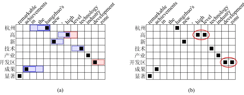
Figure 3: Example output from the ITG using non-compositional phrases. (a) is the Viterbi alignment from the word-based ITG. The shaded regions indicate phrasal alignments that are allowed by the non-compositional constraint; all other phrasal alignments will not be considered. (b) is the Viterbi alignment from the phrasal ITG, with the multi-word alignments highlighted.
5 Bootstrapping Phrasal ITG from Word-based ITG
This section introduces a technique that bootstraps candidate phrase pairs for phrase-based ITG from word-based ITG Viterbi alignments. The word-based ITG uses the same expansions for the non-terminalX, but the expansions ofC are limited to generate only 1-1, 1-0, and 0-1 alignments:
C → e/f, C → e/ǫ, C → ǫ/f
where ǫ indicates that no word was generated. Broadly speaking, the goal of this section is the same as the previous section, namely, to limit the set of phrase pairs that needs to be considered in the train-ing process. The tic-tac-toe pruntrain-ing relies on IBM model 1 for scoring a given aligned area. In this part, we use word-based ITG alignments as anchor points in the alignment space to pin down the poten-tial phrases. The scope of iterative phrasal ITG train-ing, therefore, is limited to determining the bound-aries of the phrases anchored on the given one-to-one word alignments.
The heuristic method is based on the Non-Compositional Constraint of Cherry and Lin (2007). Cherry and Lin (2007) use GIZA++ intersections which have high precision as anchor points in the
bitext space to constraint ITG phrases. We use ITG Viterbi alignments instead. The benefit is two-fold. First of all, we do not have to run a GIZA++ aligner. Second, we do not need to worry about non-ITG word alignments, such as the(2,4,1,3)permutation patterns. GIZA++ does not limit the set of permu-tations allowed during translation, so it can produce permutations that are not reachable using an ITG.
Formally, given a word-based ITG alignment, the bootstrapping algorithm finds all the phrase pairs according to the definition of Och and Ney (2004) and Chiang (2005) with the additional constraint that each phrase pair contains at most one word link. Mathematically, lete(i, j)count the number of word links that are emitted from the substringei...j,
andf(l, m) count the number of word links emit-ted from the substringfl...m. The non-compositional
phrase pairs satisfy
e(i, j) =f(l, m)≤1.
Figure 3 (a) shows all possible non-compositional phrases given the Viterbi word alignment of the ex-ample sentence pair.
6 Summary of the Pipeline
start from sentence-aligned bilingual data and run IBM Model 1 in both directions to obtain two trans-lation tables. Then we use the efficient bidirectional tic-tac-toe pruning to prune the bitext space within each of the sentence pairs; ITG parsing will be car-ried out on only this this sparse set of bitext cells. The first stage of training is word-based ITG, us-ing the standard iterative trainus-ing procedure, except VB replaces EM to focus on a sparse prior. Af-ter several training iAf-terations, we obtain the ViAf-terbi alignments on the training data according to the fi-nal model. Now we transition into the second stage – the phrasal training. Before the training starts, we apply the non-compositional constraints over the pruned bitext space to further constrain the space of phrase pairs. Finally, we run phrasal ITG tive training using VB for a certain number of itera-tions. In the end, a Viterbi pass for the phrasal ITG is executed to produce the non-compositional phrasal alignments. From this alignment, phrase pairs are extracted in the usual manner, and a phrase-based translation system is trained.
7 Experiments
The training data was a subset of 175K sentence pairs from the NIST Chinese-English training data, automatically selected to maximize character-level overlap with the source side of the test data. We put a length limit of 35 on both sides, producing a train-ing set of 141K sentence pairs. 500 Chinese-English pairs from this set were manually aligned and used as a gold standard.
7.1 Word Alignment Evaluation
First, using evaluations of alignment quality, we demonstrate the effectiveness of VB over EM, and explore the effect of the prior.
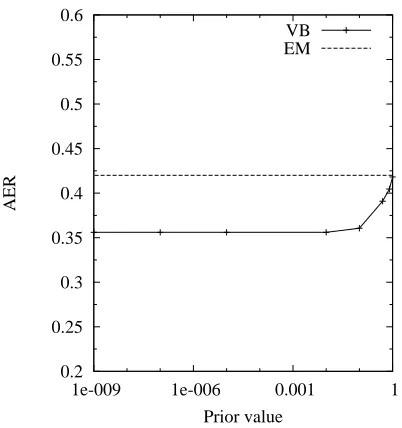
Figure 4 examines the difference between EM and VB with varying sparse priors for the word-based model of ITG on the 500 sentence pairs, both af-ter 10 iaf-terations of training. Using EM, because of overfitting, AER drops first and increases again as the number of iterations varies from 1 to 10. The lowest AER using EM is achieved after the second iteration, which is .40. At iteration 10, AER for EM increases to .42. On the other hand, using VB, AER decreases monotonically over the 10 iterations and
0.2 0.25 0.3 0.35 0.4 0.45 0.5 0.55 0.6
1e-009 1e-006 0.001 1
AER
[image:7.612.323.524.64.278.2]Prior value VB EM
Figure 4: AER drops as αC approaches zero; a more
sparse solution leads to better results.
stabilizes at iteration 10. WhenαC is1e−9, VB gets AER close to .35 at iteration 10.
As we increase the bias toward sparsity, the AER decreases, following a long slow plateau. Although the magnitude of improvement is not large, the trend is encouraging.
These experiments also indicate that a very sparse prior is needed for machine translation tasks. Un-like Johnson (2007), who found optimal perfor-mance when α was approximately 10−4, we ob-served monotonic increases in performance as α
dropped. The dimensionality of this MT problem is significantly larger than that of the sequence prob-lem, though, therefore it may take a stronger push from the prior to achieve the desired result.
7.2 End-to-end Evaluation
sig-nificant impact on the output.
We also trained a baseline model with GIZA++ (Och and Ney, 2003) following a regimen of 5 it-erations of Model 1, 5 itit-erations of HMM, and 5 iterations of Model 4. We computed Chinese-to-English and Chinese-to-English-to-Chinese word translation ta-bles using five iterations of Model 1. These val-ues were used to perform tic-tac-toe pruning with
τb = 1×10⁻³andτs= 1×10⁻⁶. Over the pruned charts, we ran 10 iterations of word-based ITG using EM or VB. The charts were then pruned further by applying the non-compositional constraint from the Viterbi alignment links of that model. Finally we ran 10 iterations of phrase-based ITG over the residual charts, using EM or VB, and extracted the Viterbi alignments.
For translation, we used the standard phrasal de-coding approach, based on a re-implementation of the Pharaoh system (Koehn, 2004). The output of the word alignment systems (GIZA++ or ITG) were fed to a standard phrase extraction procedure that extracted all phrases of length up to 7 and esti-mated the conditional probabilities of source given target and target given source using relative fre-quencies. Thus our phrasal ITG learns only the minimal non-compositional phrases; the standard phrase-extraction algorithm learns larger combina-tions of these minimal units. In addition the phrases were annotated with lexical weights using the IBM Model 1 tables. The decoder also used a trigram lan-guage model trained on the target side of the training data, as well as word count, phrase count, and distor-tion penalty features. Minimum Error Rate training (Och, 2003) over BLEU was used to optimize the weights for each of these models over the develop-ment test data.
We used the NIST 2002 evaluation datasets for tuning and evaluation; the 10-reference develop-ment set was used for minimum error rate training, and the 4-reference test set was used for evaluation. We trained several phrasal translation systems, vary-ing only the word alignment (or phrasal alignment) method.
Table 1 compares the four systems: the GIZA++ baseline, the ITG word-based model, the ITG word model using EM training, and the ITG multi-word model using VB training. ITG-mwm-VB is our best model. We see an improvement of nearly
Development Test
GIZA++ 37.46 28.24
ITG-word 35.47 26.55
ITG-mwm (VB) 39.21 29.02
[image:8.612.333.526.60.132.2]ITG-mwm (EM) 39.15 28.47
Table 1: Translation results on Chinese-English, using the subset of training data (141K sentence pairs) that have length limit 35 on both sides. (No length limit in transla-tion. )
2 points dev set and nearly 1 point of improvement on the test set. We also observe the consistent supe-riority of VB over EM. The gain is especially large on the test data set, indicating VB is less prone to overfitting.
8 Conclusion
We have presented an improved and more efficient method of estimating phrase pairs directly. By both changing the objective function to include a bias toward sparser models and improving the pruning techniques and efficiency, we achieve significant gains on test data with practical speed. In addition, these gains were shown without resorting to external models, such as GIZA++. We have shown that VB is both practical and effective for use in MT models. However, our best system does not apply VB to a single probability model, as we found an apprecia-ble benefit from bootstrapping each model from sim-pler models, much as the IBM word alignment mod-els are usually trained in succession. We find that VB alone is not sufficient to counteract the tendency of EM to prefer analyses with smaller trees using fewer rules and longer phrases. Both the tic-tac-toe pruning and the non-compositional constraint ad-dress this problem by reducing the space of possible phrase pairs. On top of these hard constraints, the sparse prior of VB helps make the model less prone to overfitting to infrequent phrase pairs, and thus improves the quality of the phrase pairs the model learns.
References
Matthew Beal. 2003. Variational Algorithms for Ap-proximate Bayesian Inference. Ph.D. thesis, Gatsby Computational Neuroscience Unit, University College London.
Peter F. Brown, Stephen A. Della Pietra, Vincent J. Della Pietra, and Robert L. Mercer. 1993. The mathemat-ics of statistical machine translation: Parameter esti-mation. Computational Linguistics, 19(2):263–311, June.
Colin Cherry and Dekang Lin. 2007. Inversion transduc-tion grammar for joint phrasal translatransduc-tion modeling. In Proceedings of SSST, NAACL-HLT 2007 / AMTA Workshop on Syntax and Structure in Statistical Trans-lation, pages 17–24, Rochester, New York, April. As-sociation for Computational Linguistics.
David Chiang. 2005. A hierarchical phrase-based model for statistical machine translation. In Proceedings of ACL, pages 263–270, Ann Arbor, Michigan, USA. Sharon Goldwater and Tom Griffiths. 2007. A fully
bayesian approach to unsupervised part-of-speech tag-ging. In Proceedings of the 45th Annual Meeting of the Association of Computational Linguistics, pages 744–751, Prague, Czech Republic, June. Association for Computational Linguistics.
Mark Johnson. 2007. Why doesn’t EM find good HMM POS-taggers? In Proceedings of the 2007 Joint Conference on Empirical Methods in Natural guage Processing and Computational Natural Lan-guage Learning (EMNLP-CoNLL), pages 296–305. Philipp Koehn. 2004. Pharaoh: A beam search
de-coder for phrase-based statistical machine translation models. In Proceedings of the 6th Conference of the Association for Machine Translation in the Americas (AMTA), pages 115–124, Washington, USA, Septem-ber.
Kenichi Kurihara and Taisuke Sato. 2006. Variational bayesian grammar induction for natural language. In International Colloquium on Grammatical Inference, pages 84–96, Tokyo, Japan.
Daniel Marcu and William Wong. 2002. A phrase-based, joint probability model for statistical machine transla-tion. In 2002 Conference on Empirical Methods in Natural Language Processing (EMNLP).
Robert C. Moore. 2003. Learning translations of named-entity phrases from parallel corpora. In Proceedings of EACL, Budapest, Hungary.
Franz Och and Hermann Ney. 2003. A systematic com-parison of various statistical alignment models. Com-putational Linguistics, 29(1):19–51, March.
Franz Josef Och and Hermann Ney. 2004. The align-ment template approach to statistical machine transla-tion. Computational Linguistics, 30(4):417–449, De-cember.
Franz Josef Och. 2003. Minimum error rate training in statistical machine translation. In Proceedings of ACL, pages 160–167, Sapporo, Japan.
Frank Soong and Eng Huang. 1991. A tree-trellis based fast search for finding the n best sentence hypotheses in continuous speech recognition. In Proceedings of ICASSP 1991.
Stephan Vogel, Hermann Ney, and Christoph Tillmann. 1996. HMM-based word alignment in statistical trans-lation. In Proceedings of COLING, pages 836–741, Copenhagen, Denmark.
Stephan Vogel. 2005. PESA: Phrase pair extraction as sentence splitting. In MT Summit X, Phuket, Thailand. Dekai Wu. 1997. Stochastic inversion transduction grammars and bilingual parsing of parallel corpora. Computational Linguistics, 23(3):377–403, Septem-ber.