Munich Personal RePEc Archive
Ordered Consumer Search
Armstrong, Mark
Department of Economics, University of Oxford
24 June 2016
Ordered Consumer Search
Mark Armstrong
June 2016
Abstract
The paper discusses situations in which consumers search through their options in a deliberate order, in contrast to more familiar models with random search. Topics include: network e¤ects (consumers may be better o¤ following the same search order as other consumers); the use of price and non-price advertising to direct search; the impact of consumers starting a new search with their previous supplier; the incentive sellers have to merge or co-locate with other sellers; and the incentive a seller can have to raise its own search cost. I also show how ordered search can be reformulated as a simpler discrete choice problem without search frictions.
Keywords: Consumer search, sequential search, ordered search, directed search, discrete choice, oligopoly, advertising, obfuscation.
1
Introduction
Consider a consumer who wishes to purchase one product from several variants available. In some cases she might know exactly what she wants in advance, and no prior market investigation is needed. In other situations, she might be so ill-informed that she stumbles randomly from one option to another until she discovers something suitable. Between these extremes, though, the consumer has some initial idea about which options are more likely to be suitable, or cheaper, or easier to inspect, and she will deliberately investigate these …rst. (She will go on to investigate other options if she is disappointed by what she …nds there.) For instance, in an online book market De los Santos, Hortacsu and Wildenbeest (2012, Table 6) report: of those consumers who searched for a book only once, 69% inspected
Amazon; of those who searched two sellers, 57% inspectedAmazon …rst, andAmazon also had a large share of the second inspections of those consumers who …rst inspected other sellers.
In more detail, there are several reasons why a consumer might choose to conduct her search for a product in a deliberate order. A consumer might have ex ante product (or brand) preferences in place from the start, and she anticipates she is more likely to like some products than others. Nelson (1970, page 312) writes that consumer search need not “be conducted at random. Prior to sampling, a consumer can obtain information from relatives and friends, consumer magazines, or even from advertising”.1 Relatedly, the
consumer might consult an intermediary to recommend a search order to her. For instance, enquiring about hotels in a city on speci…ed dates from an online travel agent may generate a list of available options ordered according to the travel agent’s ranking algorithm, and if the algorithm is good the consumer will do well to search in the suggested order.2 General
purpose search engines also aim to order their non-sponsored (organic) results according to estimated relevance to the consumer.3
Search might be directed by prices, in the sense that sellers advertise their prices to consumers in advance (for instance on the internet). When products are otherwise sym-metric consumers will then choose to inspect products in order of increasing price, and more generally prices can be used to attract consumers (which is not possible when prices are discovered after search, when a seller’s price can be used only to retain consumers who choose to inspect that seller). Search might also be directed by non-price advertising, so that consumers start their search at the seller which advertises the most heavily. Rational consumers might anticipate that the seller that spends the most on advertising will turn out to o¤er the lowest price or the most suitable product. For instance, when consumers
1In footnote 9 Nelson writes that he has a detailed theory of “guided search” which “could not be
included here because of space limitations”.
2Ursu (2015) studies such a travel agent empirically. An important feature of her dataset is that the
travel agent randomized its recommendations to some consumers, which allows her to study the e¤ect of rank on click rates and purchase decisions in a clean way. In the random order treatment, consumers clicked on links with decreasing frequency further down the page (since presumably they believe the ranking has some content) but their purchase probability contingent on clicking does not depend on page position. However, when the travel agent’s true ranking was displayed, the purchase probability did depend strongly on rank, suggesting that the ranking algorithm was indeed useful to consumers as a guide to search.
3Baye, De los Santos, and Wildenbeest (2016) document how the tra¢c generated by organic results
use a search engine it might be that the most relevant seller for them is the seller that bids the most to be displayed …rst in the sponsored search results, in which case consumers should inspect sellers in the order they appear on the results page.
If other consumers follow a particular search order, it can be optimal for an individual consumer to do the same. When many consumers search through sellers in the same order, a seller placed earlier in this order will often set a lower price than its rivals further back. A seller placed further back knows that a consumer it encounters is likely to have been disappointed in the o¤ers received so far—from the seller’s perspective, this is a form of advantageous selection—and so it can a¤ord to set a high price. In such cases, an individual consumer then does better to search in the same order as other consumers. Because of this, if other consumers use a rule of thumb for choosing which seller to inspect …rst—for example, as above they …rst inspect the seller which advertises with the greatest intensity, or even if they use a more ad hoc procedure such as searching through sellers in alphabetical order—then an individual consumer should do the same. Similarly, it may be that one seller has managed to achieve a “low price image” which induces consumers to try there …rst, and in equilibrium this seller does have an incentive to choose lower prices. This kind of self-ful…lling prophecy means that a highly skewed pattern of sales can emerge even in symmetric environments.
Some products have lower search costs than others. For instance, geography or shop layout determines a consumer’s search order, and she might choose to inspect the nearest option …rst (which might be di¤erent for di¤erent consumers). In a physical store it is easier to inspect products displayed at eye level or on the ground ‡oor, regulation might require certain products to be on the “top shelf”, while unhealthy products aimed at children might pro…tably be placed at a lower height. Judicious design of store layout might mean that a multiproduct seller can force the consumer to consider its products in a particular order. Consumers might …nd it less costly to inspect a new product from a supplier they have used before than from a new supplier, perhaps because they have contact details readily available.
choose to …rst visit a “big box” store which stocks more varieties of the product in question. However, because pricing is coordinated within the store, it is likely that the store will set a higher price than its smaller rivals, and consumers choosing their search order have to trade o¤ the one-stop shopping bene…ts of greater variety with the higher price they will have to pay there.
The rest of this paper is organized as follows. Section 2 describes the principles govern-ing optimal sequential search in fairly general terms, and shows how the search problem can be reformulated as a simpler discrete choice problem without search frictions. Section 3 uses this theory to describe outcomes in a model where sellers choose prices for their products. In simple settings where each consumer views the sellers as symmetric ex ante, this model often exhibits multiple equilibria: the consumer search order depends on which sellers choose lower prices, and the prices that sellers choose depend on where they are in the search order. Random consumer search is one equilibrium (and is often the fo-cus of existing oligopoly models), although it is often an unstable equilibrium. However, if the demand system is “smoothed”, by making individual consumers have su¢ciently heterogeneous preferences over sellers, the market might have a single equilibrium.
Extensions to this basic model are presented in section 4, which aim to illustrate several of the reasons for ordered search described above. These include discussions of how multi-seller clusters and “big box” multi-sellers should often be inspected …rst by consumers, how sellers chooses prices when they anticipate that consumers start a new search process with their previous supplier, how it might be pro…table for a seller to deliberately increase its inspection costs, and the impact of both price and non-price advertising on market outcomes. Section 5 suggests some promising options for further research. The relevant literature, much of which is very recent, is discussed as I present various aspects of ordered search in the paper.
2
Opening the box
Consider a consumer who wishes to select one product from several variants which are available. One way to model this decision problem is to suppose that the consumer knows in advance her idiosyncratic match utility for each product i, sayvi, and knows in advance
each product’s price,pi, and chooses the option with the highest net surplusvi piprovided
where before purchase the consumer needs to incur a cost si to discover product i’s
char-acteristics, vi and pi. (In section 4.5 I also study a scenario between these two extremes,
where consumers know each product’s price in advance but need to discover the associated match utility.4) The kinds of products where consumers have idiosyncratic tastes, and
which they usually wish to inspect in some way before buying (even if they know the price in advance), include cameras, cars, clothing, furniture, hotels, novels, perfume, and pets.
Before studying in the next section how equilibrium prices in an oligopoly are deter-mined, we …rst describe the risk-neutral consumer’s optimal search strategy for a given set of options. Weitzman (1979) provides the key to understanding optimal sequential search through a …nite number of mutually exclusive options (“boxes”) with uncertain payo¤s. The consumer’s payo¤ from option i is a random variable vi 0, where her payo¤s are
independently distributed across options with CDF Fi(vi) for option i. (It is natural to
suppose the payo¤ vi is non-negative if the consumer has an outside option of zero.) To
discover the realization of vi inside box i involves the non-refundable inspection cost si.
There is free recall, so that the consumer can costlessly return to claim the payo¤ from a box opened earlier. The consumer wishes to consume at most one of the options, and aims to maximize the expected value of the consumed option net of total search costs. To do this she decides both the order in which to inspect options and the rule for when to terminate search (in which case she consumes the best option opened so far). Weitzman refers to this as “Pandora’s problem”, and the consumer is female in this paper.5
For now, suppose that i Eivi > si for each i, for otherwise it is never optimal to
open boxi and this option can be eliminated from her choice problem. (Here, Ei denotes
taking expectations with respect to the distribution for vi.) De…ne the “reservation price”
of box ito be the unique price ri which satis…es
Eimaxfvi ri;0g=si : (1)
(Since i > si, this reservation price is positive.) In terms of demand theory, ri is the
highest price such that the consumer is willing to incur the sunk cost si for the right to
purchase the product at that price once she has discovered her match utility. The expected incremental bene…t of inspecting box i given that the consumer already has secured a
4The remaining con…guration, where consumers know their match utilities in advance but must incur
search costs to discover the associated prices, su¤ers from the problem of hold-up and market shut-down, as initially discussed by Diamond (1971).
potential payo¤ x 0to which she can freely return is
Eimaxfvi; xg si x=Eimaxfvi x;0g si ; (2)
which is positive if and only if her current payo¤ xis below the reservation price ri.
Weitzman shows that an optimal search strategy in this context—“Pandora’s rule”—is as follows.6
Selection rule: If a box is to be opened, it should be the unopened box with the highest reservation price;
Stopping rule: Terminate search whenever the maximum payo¤ discovered so far exceeds the reservation price of all unopened boxes (which is zero if no box remains unopened), and consume the option with this maximum payo¤.
For instance, suppose there are three boxes with respective reservation prices ri and
realized payo¤s vi given by
(r1; v1) = (5;2) ; (r2; v2) = (10;4) ; (r3; v3) = (3;7) : (3)
Then the consumer (who of course does not know the realized payo¤ vi until she opens
that box) should …rst inspect box 2 as that has the highest reservation price, should go on to inspect box 1 (since that box has reservation price above her current payo¤ v2 = 4),
then come back to consume the payo¤ in box 2 without inspecting box 3 (sincev2 is above
bothv1 and r3).
The reservation price in (1) depends only on the properties of that option, i.e., si and
Fi. The reservation price for a box is not the same as that box’s stand-alone surplus,
i si. If the consumer could only choose one box to open, she would choose the box
with the highest value of i si, which need not be the box with the highest ri.7 As is
intuitive, the reservation price in (1) is decreasing in si and increasing in [1 Fi( )]. In
addition, since it depends on the right-tail of the distribution, all else equal it is increasing in the “riskiness” of the option. As Weitzman (1979, page 647) puts it: “Other things
6The optimality of this rule depends on a number of factors. When the consumer cannot freely return
to an earlier opened box, it may not be optimal to inspect boxes in order of their reservation values. See Salop (1973) for an investigation of optimal order of search when there is no recall (which is a common assumption in the job search literature). Olszewski and Weber (2015) discuss how the rule needs to be modi…ed when the agent gains utility from all opened boxes, while Doval (2014) considers the situation where the agent can consume the contents of a box without inspecting it …rst (and without incurring the search cost).
being equal, it is optimal to sample …rst from distributions which are more spread out or riskier in hopes of striking it rich early and ending the search.”
Pandora’s rule can conveniently be re-expressed as a simpler discrete choice prob-lem without search frictions.8 Speci…cally, Pandora’s rule is equivalent to the choice rule
whereby the consumer chooses the payo¤ from the box with the highest index
wi minfri; vig ; (4)
where vi is the realized payo¤ inside boxi. (This is the case in the scenario in (3) above,
when box 2 was ultimately selected.) To see this, we show that box j is not chosen under Pandora’s rule whenwj < wi. Ifrj < ri, then boxiwill be inspected before j, andj could
then be chosen only if it is inspected, which requires vi < rj, and then only if vi < vj,
which taken together contradict the assumption wj < wi. If instead rj > ri, then box
j is inspected before i. But then wj < wi implies vj < minfri; vig, which implies that
box j is not consumed before …rst inspecting i, which then reveals a superior payo¤. In either case, the inequality wj < wi implies that box j is not chosen. Since some box is
eventually chosen under Pandora’s rule, we deduce it is the box with the highest wi. In
sum, while the box-speci…c index ri determines which box the consumer opens …rst, the
box-speci…c index wi determines which box is ultimately selected.9 As shown in Theorem
1 in Kleinberg, Waggoner, and Weyl (2016), which itself builds on Weber (1992), this reformulation of Pandora’s rule allows for the elegant proof of Weitzman’s result which is presented in Appendix A below.
When a population of consumers choose their options it will often be the case that consumers di¤er in their reservation pricerifor boxi. For instance, consumers might di¤er
in their cost of inspecting a given box (e.g., due to their di¤erent geographic locations) or in their prior distribution for a box’s match utility. An individual consumer is characterized by her list of reservation prices (r1; r2; :::) and her list of realized payo¤s (v1; v2; :::) which
via (4) generate the list(w1; w2; :::). This heterogeneous population of consumers selecting
an option via optimal sequential search can equivalently be modelled as engaging in a discrete choice problem, where the type-(w1; w2; :::) consumer simply selects the option
8This discussion develops the analysis in Armstrong and Vickers (2015, pages 303-4), where we showed
how a search problem with free recall of earlier options can be recast as a discrete choice problem without search frictions. (This reformulation is not possible without free recall of earlier options.)
9SinceE
with the highestwi. The joint distribution of(w1; w2; :::)in the consumer population then
determines the demand for each option.
3
Ordered search with strategic sellers
We now put strategic sellers inside these boxes. Suppose there are a …nite number of sellers, labelled i = 1;2; :::, which each supply a single variant of a product, where seller
i has constant marginal cost of production ci. Consumers want at most one product and
have idiosyncratic match utilities for the product from seller i, denoted vi, where vi is
not observed by the seller. A particular consumer incurs search cost si to inspect seller
i, anticipates that seller i’s match utility comes from the CDF Fi(vi) and believes that
her match utilities are independently distributed across sellers. Seller i chooses price p~i,
and a consumer who buys from i obtains payo¤ vi p~i (excluding her search costs). The
consumer discovers seller i’s price p~i and the corresponding match utility vi only after
paying the search cost si. I assume that the consumer can freely return to a previously
inspected product and there is no danger of a popular product being sold out. (These two assumptions distinguish consumer search from the typical job search model.)
-6
0 p1
[image:9.595.196.433.444.652.2]p2 r1 r2 …rst inspect seller 1 …rst inspect seller 2 p p p p p p p p p p p p p p p p p p p p p p p p p p p p p p p p p p p p p p p p p p p p p p p p p p p p p p p p p p p p p p p p p p p p p p p p p p p p p p p p p p p p p p p p p p p p p p p p p p p p p p p p p p p p p p p p p p p p p p p p p p p p p p p p p p p p p p p p p p p p p p p p p p p p p p p p p p p p
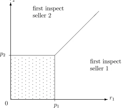
Figure 1: The optimal search order with two sellers
Since the consumer’s decision to inspect a seller, and the order in which she inspects sellers, depends on anticipated, not actual, prices, write pi for the anticipated price from
~
pi. Given a list of anticipated prices (p1; p2; :::), the consumer’s optimal search order is
described by Pandora’s rule. To understand what this means we need to calculate the reservation price of the lottery inside boxi, which has anticipated payo¤ maxfvi pi;0g.
As discussed in section 2, if pi > ri, where ri in (1) is the reservation price for the match
utilityvi, it is not worthwhile for this consumer ever to inspect selleri. If pi < ri, though,
the reservation price of the box with payo¤ maxfvi pi;0g and search cost si is positive
and equal to ri pi.10 Therefore, according to Pandora’s rule this consumer should …rst
inspect the seller with the highest ri pi, if this is positive, and keep searching until her
maximum sampled payo¤ vk p~k (where p~k is seller k’s actual price) is above all of the
rj pj for uninspected products. In general, consumers will di¤er in their reservation
prices, and Figure 1 depicts the optimal search order with two sellers in terms of the pair
(r1; r2). In particular, a consumer’s decision about which seller to inspect …rst is akin to
a discrete choice problem where a consumer values option i at ri and chooses the option
with the highest payo¤ri pi (or, as shown in the shaded region, the outside option zero
if that is superior to engaging in search).
While her search order depends on anticipated prices(p1; p2; :::), a consumer’s purchase
decision depends also on the actual prices (~p1;p~2; :::). Since the payo¤ from purchasing
from seller i is vi p~i, the discrete choice reformulation in section 2 shows that seller i’s
demand is the fraction of consumers for whom the index
minfri pi; vi p~ig (5)
is positive and higher than the corresponding index from all rival sellers. For a given list of anticipated prices, this determines demand for the various sellers in terms of their actual prices. Equilibrium in this market occurs when the Bertrand equilibrium in actual prices(~p1;p~2; :::)given anticipated prices(p1; p2; :::)coincides with these anticipated prices.
Equivalently, returning to the underlying search formulation, equilibrium occurs when (i) consumers choose their order of search optimally given the prices they anticipate sellers choose, and (ii) each seller chooses its price to maximize its pro…t given the consumer search order and the prices chosen by rival sellers, and this price coincides with the price anticipated by consumers.
From (5), a seller competes against its rivals (and the outside option) on two margins. If a consumer’s preferences satisfy ri pi > vi p~i, it is the size of the latter term
10The reservation price of this box is thexwhich satis…es
which determines whether or not this consumer will buy from the seller, and the seller can a¤ect this likelihood via its choice of price p~i. Otherwise, though, it is the former
term which determines its demand, and this portion of demand is inelastic. If search costs become negligible, this oligopoly model converges to an oligopoly model where consumers have complete information about match utilities (v1; v2; :::) and actual prices (~p1;p~2; :::).
Intuitively, the …rst term ri pi in (5) is rarely relevant when the search cost for seller i
is small, and this seller sells when vi p~i is positive and higher than the corresponding
surplus from rivals.
To illustrate, consider an example with two sellers and costless production. Each con-sumer has match utility vi for product i = 1;2 which is uniformly distributed on the
interval[0;1]and has reservation priceri for this product which is also independently and
uniformly distributed on [0;1]. (From (1), the search cost corresponding to ri is given by
si = 12(1 ri) 2
and so lies in the interval[0;1
2].) Thenwi in (4) is the minimum of two
in-dependent uniform variables, and so has support[0;1]and density2(1 wi). Among those
situations where both sellers are active, this example has a unique equilibrium and in this equilibrium each seller chooses price p 0:49.11 (Details for this example are presented in
Appendix B below.) As in Figure 1, if a consumer searches at all she will …rst inspect the seller for which she has the higherri. Each consumer searches in a deterministic order, but
that order di¤ers across consumers.
If this example is modi…ed so that all search costs are zero—in which case ri 1
and wi in (5) is uniformly distributed on [0;1]—the symmetric equilibrium price is p =
p
2 1 0:41, which is below the corresponding price with search frictions. It is intuitive that more signi…cant search frictions will tend to increase equilibrium prices. Consider a particular seller in the market. If the inspection costs for this seller rise, it will tend to encounter fewer but more “desperate” consumers who have not found a good option from other sellers, and this will typically give it the opportunity to raise its price. Likewise, if the inspection costs for its rivals increase, this reduces the distribution for rj, and hence
wj, from rivals and again this tends to give the seller an incentive to raise its price. In
sum, if inspection costs rise, either for a single seller or across the market, this is likely to
11As usual, there are also less interesting equilibria in which consumers anticipate that sellerichooses
such a high price that it is not worthwhile to inspect this seller, and then this seller has no way to attract consumers to it and might as well set this very high price. In this example, for instance, there is also an equilibrium where seller 1 sets pricep1= 1and no one inspects it, while seller 2 sets the monopoly price
raise each seller’s equilibrium price.
The “double uniform” example above involves a demand system which is smooth, in the sense that small changes in anticipated pricespido not lead to discrete changes in demands.
In other situations—which include those commonly studied in the literature—the demand system is not smooth. Speci…cally, consider the situation in which each consumer considers sellers to be symmetricex ante, so that (in the duopoly case) reservation prices on Figure 1 lie on the45o line. Here, when one seller is expected to o¤er a lower price,all consumers
who search will choose to inspect it …rst. There is a strong possibility of multiple equilibria in such a market: the consumer search order depends sensitively on anticipated prices, while a seller’s price usually depends on where it is placed in the search order.
To discuss this point in more detail, suppose each consumer has the same CDF F(v)
for match utility and the same inspection cost s from each seller, and hence has the same reservation price r for each seller’s product. Suppose also that each seller has the same production cost c. This is the framework analyzed in the in‡uential models of Wolinsky (1986) and Anderson and Renault (1999), under the assumption that consumers search randomly through sellers. In contrast to these earlier papers, suppose instead that all consumers search through sellers in the same order.12 If the hazard rate for match utility,
f(v)=(1 F(v)), is strictly increasing inv, then more prominent sellers (i.e., sellers closer to the start of this search order) have more elastic demand than those sellers placed further back. For this reason, more prominent sellers typically set lower prices, which in turn rationalizes the assumed consumer search order. Intuitively, a seller inspected earlier in a consumer’s search order knows that a prospective consumer is likely to have a superior outside option relative to the situation where a seller is inspected later—a later seller only encounters a consumer if that consumer was disappointed by her options so far—and with an increasing hazard rate, a seller who knows a consumer has a better outside option will choose to set a lower price. A more detailed argument for why a prominent seller faces more elastic demand is presented in Appendix C below.
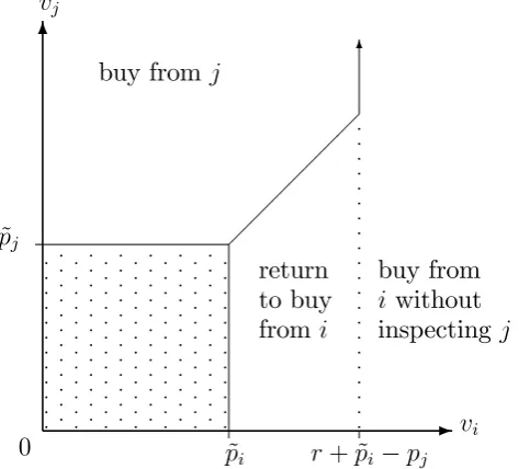
To see how ordered search can be an equilibrium in a symmetric environment, suppose there are two symmetric sellers and look for an equilibrium wherepi < pj so that selleri is
inspected …rst by all consumers. Here, the pattern of demand for the two sellers is shown
12The following discussion is based on the analysis (for the uniform distribution) in Armstrong, Vickers,
in Figure 2.13 Appendix D below calculates equilibrium prices for various search costs when production is costless and match utility is uniformly distributed, and shows how the prominent …rm indeed chooses a lower price in equilibrium (see Figure 4 in the appendix). Thus there are two equilibria with ordered search, one where all consumers inspect seller 1 …rst and one where they inspect seller 2 …rst. There is also a third, symmetric, equilibrium, where exactly half the consumers …rst inspect each seller and where the two sellers set the same price. However, this symmetric equilibrium—which is the focus of the analysis in Wolinsky (1986) and Anderson and Renault (1999)—isunstable: if slightly more consumers …rst inspect one seller, that seller chooses to set a lower price than its rival, so that all consumers will strictly prefer to visit that seller …rst. Thus, this is a classic “tipping” market, and we expect one low-price seller will be inspected …rst by all consumers even though sellers are symmetric ex ante.14
-6
r+ ~pi pj
6
0 p~i
~ pj vi vj buy from i without inspecting j return to buy fromi
buy fromj
[image:13.595.197.434.345.559.2]p p p p p p p p p p p p p p p p p p p p p p p p p p p p p p p p p p p p p p p p p p p p p p p p p p p p p p p p p p p p p p p p p p p p p p p p p p p p p p p p p p p p p p p p p p p p p p p p p p p p p p p p p p p p p p p p p p p p p p p p p p p p p p p p p p p p p p p p p p p p p p p p p p p p p p p p p p p p p p p p p p p p p p p p p p p p p p p p p
Figure 2: Demand for the two sellers when pi < pj
Consumers may well be worse o¤ in an equilibrium with ordered search where they all inspect one seller …rst compared to the equilibrium with random search.15 Intuitively,
13This pattern is generated by observing that a consumer buys from seller i if minfr p
i; vi p~ig is positive and greater thanminfr pj; vj p~jg.
14In situations where the hazard rate is decreasing, a seller which is …rst inspected by more consumers
sets a higher price than its rival, and the unique and stable equilibrium has the two sellers setting the same price and half the consumers …rst inspect each seller. (In the knife-edge case of an exponential distribution for match utility, where the hazard rate is constant, a seller’s price does not depend on where it is in the search order, and no network e¤ects are present.)
15Armstrong, Vickers, and Zhou (2009) and Zhou (2011) show this to be so in the case with a uniform
faced with the increasing price path which goes with ordered search, consumers cease their search too early and competition between sellers is weakened. In this market with ordered search, the seller which inspected …rst has larger demand for two reasons: even with equal prices its demand would be larger because it is inspected …rst (its extra demand the “north-east” region on Figure 2), while its lower price reinforces this e¤ect. The result is that the distribution of sales across sellers is more skewed than it would be in a market with random search or in a market without search frictions. In the example analyzed in Appendix D, sales are equal for the two sellers when search frictions are absent, but the prominent seller sells up to twice as much as its rival when search costs are larger. As search frictions increase, we expect that the prominent seller’s sales volume increases, while the non-prominent seller’s sales volume will fall (see Figure 5).
In this market where sellers are symmetric ex ante, in the stable equilibrium where all consumers visit one prominent seller …rst this seller makes greater pro…t than its rival. (The prominent sellercould choose the equilibrium price of its rival, in which case it has greater demand and more pro…t, but in general is even better o¤ with another price.) The impact on pro…t of an increase in search frictions will often di¤er for the two sellers.16 Pro…t for
the prominent seller will rise withssince both its price and its demand do. The impact on the non-prominent seller’s pro…t, though, depends on two opposing forces—its price rises, but its demand is likely to fall—and the result is that its pro…t can be non-monotonic in the search cost (see Figure 6). When there are no search frictions both sellers choose the same price and obtain the same pro…t. Assincreases both sellers’ pro…ts initially rise, but for largersthe non-prominent seller’s pro…t falls as search frictions increase. In this second region, less prominent sellers will favour consumer policy which reduces search frictions, while such a policy would be opposed by more prominent sellers.
The existence of multiple equilibria can make it hard to do comparative statics, such as whether a higher-quality …rm (where the match valuation distribution comes from a better CDF) sets a higher price or is inspected …rst or whether a …rm with a higher inspection cost is inspected later. For this reason a smooth demand system, where di¤erent consumers prefer to search in di¤erent orders, might work better (as well as often being more plausible). However, such a model can be cumbersome to work with beyond speci…c
search relative to the price with random search, provided there are at least four sellers.
16See also the discussion and Figure 2 in Zhou (2011). By contrast, with random search (and no outside
examples or without resorting to numerical methods.
One convenient way to simplify this framework is to study monopolistic competition with many symmetric sellers (Wolinsky, 1986), when a stable equilibrium with symmetric prices exists in a broad class of cases.17 When a consumer expects all sellers to o¤er the
same price p < r, a consumer will search until she …nds a product with v r and will never return to a previous seller.18 Thus a seller has no “return demand”, which was the
source of the incentive for prominent …rms to set lower prices, and a seller sets the same price regardless of its place in the search order. The result is that consumers do not care how other consumers choose to search, and there is no tendency to tip. The symmetric equilibrium price,psay, when consumers are also symmetric is derived as follows. Consider a seller who meets a consumer. If it chooses price p~ the consumer will buy from it if
v p~ r p, and so the seller’s pro…t from this consumer is(~p c) [1 F(~p+r p)]. In equilibrium, this must be maximized atp~=p, which yields the unique …rst-order condition
p=c+1 F(r)
f(r) : (6)
The equilibrium markup and industry pro…t in this market, (1 F(r))=f(r), depends on the shape of the CDF F(v) and the magnitude of search frictions. Consumers have an incentive to participate in this market provided that p in (6) is below r. When the hazard rate f =(1 F) increases, the equilibrium price in (6) decreases with r and hence increases with the search cost s. In such cases, a reduction in search frictions yields a double bene…t to consumers: their average match utility is higher and the price they pay is lower. Although this model of monopolistic competition does not necessarily involve ordered search, it is useful starting point for some of the applications and extensions to this basic framework presented in the next section.
17Anderson and Renault (1999) show that a symmetric equilibrium with monopolistic competition exists
provided that the hazard rate is increasing.
18Anderson and Renault (2015) discuss another way to obtain this simplifying feature. They suppose
4
Applications and extensions
4.1
Mergers and clusters
There are a number of situations in which consumers incur a single search cost to inspect several products at once. For instance, a single seller might stock several product variants, or several single-product sellers might cluster in a single location. Unless the equilibrium price is signi…cantly higher in a multiproduct location, consumers may then choose to inspect such a location before any of the single-product locations.
To discuss this in more detail, consider a situation with monopolistic competition, where a large number of ex ante symmetric sellers each supply a single variant of the product, so that the equilibrium price is given byp in (6). Suppose that two of these sellers merge to form a “big box” seller which supplies two of the product variants. When a consumer inspects this seller, she incurs the same search costs as with any other seller but sees two options (each with an independent match utility from the CDF F(v) and an associated price), from which she will select the better one if she buys from this seller.19 In regular
cases, the merged …rm will choose the same price for each variant, and so this seller can be considered to be another single-product …rm but one that has a better CDF for its match utility given by F2
instead of F. Typically, the merged …rm will adjust its price upwards relative to its rivals, which in this monopolistic competition framework continue to set the same price p. To understand this, observe that when the merged …rm meets a consumer it will sell when its match utility and price satisfy v p~ r p, and so it chooses p~to maximize(~p c)[1 F2
(~p+r p)]. One can check that its pro…t is increasing atp~=p—the demand function [1 F2
(~p)] is less elastic than[1 F(~p)]—and the big box store will set a higher price than its single-product rivals.
Whether a consumer has an incentive to inspect this merged …rm …rst depends on how high its price is. If its price does not rise by too much, a consumer will wish to inspect this multiproduct seller …rst, in which case the merger is pro…table. For instance, in the example wherev is uniformly distributed on[0;1], the search cost iss= 1
32 and production
is costless, thenr = 3
4 andp= 1
4 in (6). The reservation price for the merged …rm’s match
utility can be calculated to be about 0.817 and its price to be 0.268. Since the di¤erence between these is greater thanr p= 1
2, it is optimal for consumers to visit the merged …rm
19Section 4.2 discusses issues of intra-…rm search and store layout, which are sidestepped by the
…rst. The better chance of …nding a good product in the big store outweighs the higher price the consumer must pay there.20 More generally, a group of sellers …nds it pro…table
to merge if the merger serves to attract consumers to visit the merged …rm …rst, and this can only be the case if consumer surplus rises as a result of the merger. Thus, in this framework there is a tendency for pro…table mergers to bene…t consumers, in contrast to the situation in many other oligopoly models.
This discussion is a simpli…ed version of the model studied in Moraga-Gonzalez and Petrikaite (2013). That paper discussed the case of oligopoly rather than monopolistic competition, and showed that a merger which results in search economies can be pro…table for the merging …rms but reduces the pro…t of non-merging …rms since they are pushed further back in the consumer search order.21 This contrasts with a more standard analysis
of Bertrand price competition, where a merger typically raises the pro…ts of non-merging …rms.
Related issues arise when one seller decides to co-locate with another seller. To discuss this point further, suppose that when this occurs a consumer pays the single search costs
to visit the cluster, where she then observes both …rms’ prices and match utilities. Unlike the case with a merger, here sellers in the cluster do not coordinate their pricing, and a seller aims to attract business from its neighboring rival as well as to prevent a consumer from leaving to inspect other locations. Provided the hazard rate is increasing, intra-cluster competition will typically mean that the price is lower in the cluster than elsewhere. If its rival sets pricep0 and o¤ers match utilityv0, then a seller which sets pricep~and o¤ersv will
sell ifv p~ maxfv0 p0; r pg. (By contrast, a seller on its own will sell under the weaker
condition v p~ r p, so that its potential consumers have a worse outside option than those of a seller in the cluster). In the uniform example discussed in the merger scenario, one can check that the equilibrium price in the two-seller location is about0:232, which is
20Ifmany single-product sellers merge, however, then a consumer is almost sure to …nd a product with
almost the maximum possible match utility, and so consumers essentially know their match utility from this seller. This implies that Diamond (1971)’s paradox applies, and the seller will set a price which just deters onward search, and this gives the consumer no incentive to incur the search cost to visit this very large store. (See Villas-Boas (2009) for related analysis in a monopoly context.) It may take many products for this e¤ect to operate, however. In the example in the text, if the large store contains 50 product variants it is still worthwhile for the consumer to inspect this seller …rst, even though its price is nearly double that of single-variant sellers.
21One advantage of using a monopolistic competition framework is that the problem of multiple equilibria
belowp= 1
4. Therefore, since consumers obtain a better distribution for their match utility
and a lower price, they will all choose to visit the cluster …rst. Because of this new-found prominence, both of the sellers there are better o¤ despite the tougher competition they face in the shared location.
A number of papers have discussed a seller’s choice between a concentrated location alongside other sellers, which attracts many consumers but where competition may be …erce, and having a more isolated location which allows the seller to exploit the few con-sumers who do pass through. These papers discuss the equilibrium con…guration of sellers, including when it is an equilibrium for all sellers to locate in a single cluster.22 The paper
closest to my discussion above is Fischer and Harrington (1996), who present a model with di¤erentiated products, one cluster location and many “peripheral” sellers, and con-sumers who choose their search order based on rational expectations of prices chosen by sellers in the cluster and by peripheral sellers and their own idiosyncractic search costs. They also document empirically which product sectors around Baltimore are more prone to clustering: shoes and antiques, where consumers like to inspect products before buying, tend to co-locate, whereas gasoline stations are more dispersed. Because of the advantages of clustering in terms of attracting consumers, a seller may be willing to sell its product through an electronic platform which also serves rivals, even though it faces strong price competition there and usually has to pay listing fees to the platform.23
4.2
Deliberate obscurity
In Fischer and Harrington (1996), …rms could choose to locate in the cluster or in the periphery. Some …rms choose the latter, in part because some consumers have search costs such that they only wish to inspect …rms in the periphery. Another issue of interest is whether it might ever be pro…table for a …rm deliberately to raise its own inspection cost—that is, to “obfuscate”—in order to make its rival the prominent seller. For instance, in the UK some well-known insurance companies advertise that their products do not
appear on price-comparison websites.
To discuss this in more detail, suppose the initial situation is that there are two
sym-22For instance, see Stahl (1982), Wolinsky (1983), Dudey (1990), Non (2010) and Ellison, Fudenberg,
and Mobius (2004). Scitovsky (1950, page 49) writes: “the geographical concentration of the expert’s market [...] should not be considered data, as Marshall did. [It is] the result of a deliberate e¤ort on the part of producers [...] in response to the expert buyer’s demand for easy comparability”.
metric sellers and are no search frictions (so the market is a duopoly version of Perlo¤ and Salop, 1985). Then consumers will investigate both sellers’ o¤ers and buy from the seller with the higher vi pi (if this is positive). In regular cases the equilibrium will be
symmetric, and …rms obtain equal pro…t. If one …rm now arti…cially introduces a positive inspection cost, s >0, this will induce all consumers to inspect the rival …rst (since they have nothing to lose by doing so). The new equilibrium prices will, given an increasing haz-ard rate, involve the prominent rival choosing the lower price, which reinforces consumer incentives to inspect this …rm …rst. However, this lower price will typically still be higher than the equilibrium price without search frictions, and this could compensate the obfus-cating seller for its disadvantaged position. As discussed in section 3, the non-prominent …rm has an incentive to raise its price since the consumers it encounters are not satis…ed with their o¤er from the prominent seller, and because prices are strategic complements this induces the prominent …rm to raise its own price too. For instance, consider the ex-ample depicted on Figure 6 below. When one …rm introduces a small inspection cost (i.e., reduces its reservation priceri), the equilibrium pro…ts are as shown on this …gure, and we
see that a small inspection cost boosts the obfuscating …rm’s pro…t a little (although the rival’s pro…t is boosted more).
Wilson (2010) analyzes this question using a di¤erent duopoly model with a homoge-neous product. There are two kinds of consumers: those who can see both prices without cost (even with “obfuscation”), and those who must pay the obfuscation costs arti…cially introduced. In this market with a homogeneous product, without obfuscation there is Bertrand competition and zero pro…t. Wilson shows that it is always in a …rm’s interest to obfuscate, with the result that …rms choose their prices according to an asymmetric mixed strategy, costly searchers inspect the transparent …rm …rst, and both …rms make positive pro…t. One di¤erence between Wilson’s model and the one presented here is that in my model the obfuscating …rm sets a higher price, while in Wilson’s model that …rm (on average) sets a lower price.24
The previous example was rather delicate, and a seller had only a small incentive to
24Ellison and Wolitzky (2012) also study a model with a homogeneous product but where consumers do
obfuscate. More striking and robust results are seen in the context of a multiproduct monopolist considering how best to price and present its products. For simplicity, consider a situation where the seller has costless production and supplies two symmetric products, 1 and 2, where each consumer’s match utility for product i is an independent draw from the CDF F(v). (The argument which follows is strengthened with asymmetric products, since then the seller can use arti…cial search frictions to divert demand from low-margin to high-margin products.) Suppose that unless the seller deliberately obfuscates, a consumer observes both prices and both match utilities from the start, and chooses the product with the higher surplus vi pi (if this is positive). In regular cases, the seller will then choose
the same price for both products, which is chosen to maximize p[1 F2 (p)].
However, the seller can always do better than this by making one product, say product 2, costly to inspect, while leaving product 1 costless to inspect (which is therefore inspected …rst by all consumers). Indeed, we will see that the seller can then obtain as pro…t the maximum value of
p1[1 F(p1)] +F(p1)p2[1 F(p2)] : (7)
Here, (7) represents the pro…t obtained if the seller could …rst o¤er product 1 to the consumer, at price p1, and the consumer chooses whether or not to buy this product
myopically, without considering the subsequent option to buy product 2. Since the pro…t in (7) coincides with the “frictionless” pro…tp[1 F2
(p)]with uniform prices p1 =p2 =p,
it is clear that the maximum pro…t in (7) is above the maximum pro…t without obfuscation. Maximizing (7) involves choosingp2 =pM, where pM is the monopoly price for a single
product, i.e., which maximizes p[1 F(p)]. Suppose the seller makes the consumer incur the search cost s for the second product so that a consumer just willing to inspect this product when priced at pM if she has no other option, so that s satis…es
s=Emaxfv pM;0
g : (8)
Suppose also that the seller chooses its prominent price p1 to maximize (7) givenp2 =pM,
which implies p1 > pM = p2. Although consumers cannot observe p2 in advance, it is an
equilibrium for consumers to anticipate the price p2 =pM and for the seller to maximize
its pro…t by choosing this price. (If consumers anticipate p2 = pM, and have to incur the
the …rst price, p1. Therefore, no consumer will ever return to buy the …rst product if they
inspect the second, and so the seller chooses p2 maximize its pro…t as if it only sold this
single product.)
In sum, it is a credible strategy for the seller to choose the two prices p1 and p2 which
maximize (7) and to introduce the arti…cial inspection cost s de…ned in (8) for product 2, and this strategy generates higher pro…t than the situation without search frictions. This policy involves an expensive product being prominently displayed, perhaps at eye level, while a cheaper product is deliberately displayed inconveniently and the consumer has to look “high and low” for a good deal. Somewhat akin to the model in Deneckere and McAfee (1996), where a seller deliberately reduces the quality of one product variant in order to facilitate price discrimination, here the seller chooses to “damage” its retail environment. In regular cases, the prominent product’s price p1 will rise while the obscure product’s
price p2 falls, relative to the situation without search frictions.25 In such cases, consumers
are harmed by the obfuscation policy: the search cost (8) eliminates all consumer surplus from product 2, while the price for product 1 is increased.
I presented here a simple variant of the model in Petrikaite (2015), who analyzes cases with more products, with asymmetric products, and with competition between multiprod-uct sellers. For instance, she shows that when prodmultiprod-ucts di¤er in quality, the seller will choose to obfuscate the lower quality product. Gamp (2016) studies a related model where all prices are observed by consumers from the start, and the seller can choose to make it harder to inspect a product’s match utility. Among other results, he shows by example that obfuscation of this form can increase total welfare: the bene…ts of the low price for the obscure product outweigh the extra search costs incurred.
4.3
Repeat business
In markets with ordered consumer search, tiny asymmetries between sellers can translate into major di¤erences in their pro…ts. There is a signi…cant advantage to a seller being placed early in the consumer search order, simply because it meets more consumers than its rivals placed further back. Since consumers in symmetric situations are
indi¤erent about which seller to inspect …rst, it does not take much inducement to favour one seller in the search order, which then causes that seller to enjoy a discrete jump in its sales and pro…t. For instance, consider the case of monopolistic competition, where the equilibrium price from each seller is (6) regardless of the search order. With random search each seller obtains negligible sales and pro…t, while if one seller manages to be placed …rst in the search order—perhaps because it is slightly easier to inspect or it has a slightly superior CDF for match utility—its pro…t jumps to
(p c)[1 F(r)] = [1 F(r)] 2
f(r) : (9)
One way to introduce small asymmetries between sellers is to consider a framework where sellers supply various products over time and consumers purchase repeatedly. (This discussion is taken from Armstrong and Zhou, 2011, section 3.) Here, it seems plausible that a consumer who previously purchased from one seller might …rst inspect the same seller when she searches for a second product, even if there is no correlation in her match utilities for the various products.26 For instance, she may have the contact details of this
seller to hand. In this case, the supplier of one product to a consumer becomes prominent for that consumer when she starts the search process for the next product.
In more detail, suppose there are two product categories, 1 and 2, which consumers buy sequentially—for instance, a bank account …rst and then a mortgage—each of which is supplied by many sellers in monopolistic competition. For product category i = 1;2, the reservation price is ri, the CDF for the match utility is Fi(v), the production cost
is ci, while the factor sellers use to discount pro…ts from the second product when they
supply the …rst product is . As in expression (9), when a supplier sells product 1 to a consumer, that consumer will go on to generate pro…t from the second product equal to
[1 F2(r2)]2
=f2(r2), and anticipating this pro…t the equilibrium price for the …rst product will be
p1 =c1+
1 F1(r1)
f1(r1)
[1 F2(r2)]2
f2(r2) :
(All sellers set the same price for the second product.) Thus, the promise of pro…t from the second product induces …rms to lower the price for the …rst product, perhaps to below its cost. When search frictions are larger for the second product, this will usually lead …rms
26If a consumer’s match utilities for a given seller’s products were positively correlated, then presumably
to o¤er a lower price for the …rst product. This outcome is reminiscent of markets with switching costs. When switching costs are small, though, they have little impact on the outcome, while here a tiny “default bias” leads to large e¤ects, and these e¤ects bene…t consumers.
Garcia and Shelegia (2015) present a related model, where a consumer is inclined to start her search process at a seller where she has observed someone else make a purchase. Again, because making a sale makes the seller prominent in a consumer’s mind, albeit a di¤erent consumer’s mind, sellers have an incentive to price low in equilibrium.
4.4
Non-price advertising
Non-price advertising can be used by sellers to achieve prominence if consumers are more likely to …rst inspect those sellers which advertise most heavily. This consumer behaviour might stem from psychological factors, if consumers most easily recall sellers from which they have seen adverts. Alternatively, rational consumers could use advertising intensity as a means by which to coordinate on their search order or as a means to choose which seller is more likely to provide a suitable product.
Consider …rst a situation with rational consumers who use advertising to coordinate on their …rst seller, anticipating that the price will be lower from the seller which spends the most on advertising. (As discussed in section 3, of the hazard-rate condition holds and sellers are symmetric ex ante, when a fraction of consumers use the rule of thumb of …rst inspecting that seller which advertises the most, that seller will choose a lower price and it is optimal to mimic that search order.) Consider a two-stage framework where two risk-neutral sellers …rst choose their advertising intensities and then choose their prices. Let H be a seller’s equilibrium pro…t (excluding advertising costs) in the second stage if
it is prominent and let L< H be the corresponding pro…t for the non-prominent seller.
The …rst stage, in which sellers compete to become prominent by advertising the most, is then a symmetric all-pay auction with complete information.27 It is clear that no pure
strategy equilibrium for advertising can exist, since spending a little more than your rival on advertising generates a discrete jump in pro…t. However, a simple symmetric mixed strategy equilibrium for advertising exists. If H(a) denotes the equilibrium probability
27See Barut and Kovenock (1998) for further analysis of this auction. A very similar model to the one
that a seller spends less than a on advertising in the …rst stage, a seller’s expected pro…t when it spends a on advertising is
H(a) H + [1 H(a)] L a : (10)
(With probability H(a) it wins the contest and enjoys high pro…t H, and otherwise it
becomes the less prominent seller.) Since a seller can obtain pro…t Lby not advertising at
all, in equilibrium pro…t in (10) must be identically equal to Lover the range of advertising
used, so thatH(a) = a
H L for 0 a H L. Thus in equilibrium each seller chooses
its advertising according to the uniform distribution on the interval [0; H L].28 The
seller which advertises more will o¤er the lower price. Each seller spends 1
2( H L) on
advertising on average, and since we expect that the bene…t of prominence, H L, is
higher when the search costsis higher (for instance, see Figure 6), this model suggests that there is more advertising in markets with higher search frictions. Competition to advertise the most acts to dissipate pro…t so that sellers earn average pro…t equal to the low level associated with not being prominent, L, which as shown on Figure 6 can decrease with
the search cost s.
This analysis is similar to Bagwell and Ramey (1994), who analyze a model where sellers o¤er a homogeneous product and consumers must choose from where to buy before they observe the seller’s choice of price. Because sellers in their model have increasing returns to scale, when more consumers turn up to buy from a seller that seller o¤ers a lower price. Thus, consumers bene…t from coordinating on a seller, and a fraction of consumers rationally go to the seller which advertises the most heavily as the means with which to do this. By contrast, the model above assumes no economies of scale but instead uses the feature that sellers who attract more …rst visits have more elastic demand. Bagwell and Ramey (1994) also report empirical studies (for eye-glasses, liquor, and prescription drugs) which show how prices were lower and market structure was more concentrated in markets where advertising was permitted, even when prices could not be advertised.
Haan and Moraga-Gonzalez (2011) analyze a related model, but where a seller’s share of …rst-inspections is continuous in its choice of advertising intensity instead of the “winner take all” formulation discussed here. They focus on a symmetric equilibrium where sellers
28Of course, here and elsewhere in this section another equilibrium exists: consumers do not respond to
advertise with the same intensity, obtain the same share of initial searches, and so charge the same price. Their model involves behavioural rather than fully rational consumers: if one seller advertises slightly more heavily than its rival and this induces more consumers to inspect it …rst, that seller will charge a lower price and hence all consumers should rationally visit that seller …rst.
An alternative scenario involves advertising intensity being associated with the most suitable, rather than the cheapest, products. For instance, consider a stylized setting where prices are not modelled and sellers di¤er in how many consumers …nd their products suitable. Speci…cally, a type-q seller o¤ers a product which each consumer has probability
q of …nding suitable, in which case the consumer obtains payo¤ 1, and with remaining probability 1 q she obtains payo¤ zero, while a seller obtains payo¤ 1 each time its product is sold. Here, sellers di¤er only in their probability of being suitable, q, which is private information and generated by the continuous CDFG(q) with support[qmin; qmax].
Suppose a consumer’s search cost ssatis…es 0< s < qmin, so that this cost is small enough
that a consumer always wishes to inspect another seller if she has not yet found a suitable product. To minimize her search costs, a consumer would like to inspect sellers in order of decreasing q if she could identify that order.
One could study this market when, as above, a seller’s advertising is simply “broad-cast” without mediation and consumers …rst inspect the seller which advertises the most heavily. However, it is perhaps implausible that consumers can really detect accurately which seller advertises the most heavily, especially when sellers advertise a similar amount. An alternative scenario involves sellers paying to be advertised on a search engine, where the seller who chooses to pay more is listed higher up the sponsored results page (which is a transparent signal for consumers to observe). Provided that better sellers do choose to pay more, it is optimal for consumers to inspect sellers—that is, to click on their links—in the order they appear on the results page.29 If a consumer clicks on its link a seller will
obtain payo¤ 1 with probability q, and soq is the value of a click to the type-q seller. In broad terms, sponsored search auctions allocate sellers to prominent positions, re-quire sellers to pay the search engine fee each time a consumer clicks on their link, and use a second-price auction format. In more detail, consider the situation with just two sellers.
29Note that in this framework the top link is not intrinsically easier to inspect. It may be more realistic
These sellers are invited to submit sealed bids, the higher bidder is listed …rst and pays the bid of the losing seller on a per-click basis, while the losing seller pays nothing but is placed second on the page. We look for a symmetric equilibrium in which the type-q
seller bids B(q), where B( ) is a strictly increasing function. Such a bidding function can be derived using standard auction techniques. Suppose that the type-q seller bids as if it had type q0, i.e., bids B(q0), while its rival has uncertain type q~and bids B(~q), in which
case the seller is listed …rst whenq < q~ 0. When it is listed …rst, consumers inspect it …rst
and so it sells to a consumer with probability q. If it loses the auction it is placed second, in which case it sells when the rival doesn’t sell and when its own product is suitable, i.e., with probability (1 q~)q. Putting this together implies the seller’s expected pro…t when it bids B(q0) is
Z q0
qmin
[q B(~q)]dG(~q) +
Z qmax
q0
[(1 q~)q]dG(~q) ;
and di¤erentiating this expression with respect to q0 and setting q0 = q reveals that the
equilibrium bid function is
B(q) =q2
: (11)
Here,q2
is the incremental pro…t for a type-qseller from being in the …rst versus the second position when its rival also has type q. Since the bidding function (11) is increasing, the more suitable seller is willing to pay more for the right to be listed …rst, with the result that consumers rationally sift through their options in the order they appear on the search engine’s results page. In this setting, the observation that consumers click more often on results placed higher up the sponsored results page is driven by the information content of the ordering, rather than “inert” consumers who blindly follow the suggested order.
This discussion of advertising on a search engine is a simple variant of Athey and Ellison (2011).30 As they put it (page 1215): “a search engine that presents sponsored
links should be thought of as an information intermediary that contributes to welfare by providing information (in the form of an ordered list) that allows consumers to search more e¢ciently”. Instead of the sealed bid format discussed here, they study an ascending bid auction in which bidders observe how many bidders remain in the auction when they decide when to drop out of the bidding. They allow for an arbitrary number of sellers, and consumers have heterogeneous search costs. Unlike the model presented above, this means that consumers face a complex decision about whether to click on one more link if they
have not been successful so far in their search. They also analyze auction design issues such as the choice of a reserve price.
Armstrong, Vickers and Zhou (2009, section 3) present a model of monopolistic compe-tition, with endogenous prices, when sellers di¤er in the quality of the product they supply (in the sense that their distributions for match utilities are ordered in terms of …rst-order stochastic dominance). In a speci…c setting with uniform distributions for match utility, we show that the highest-quality seller is willing to pay the most to become prominent, and that consumers have an incentive to inspect this seller …rst (even though it chooses a higher price than other sellers). As with sponsored search, a seller’s ability to compete for a prominent position can guide consumers towards better, and better value, products.
The models presented in this section provide the “best case” for non-price advertising to be used to guide search: the seller which is willing to pay the most to achieve prominence is the seller which consumers would like to inspect …rst. In other situations, this coincidence of interests need not hold perfectly or at all, and advertising is then a less reliable guide for consumers. For example, in the model of sponsored search, sellers might di¤er both in their likelihood of being suitable and in their expected pro…t from a click. In such a setting, the seller which is willing to bid the most per-click is not always the seller which the most consumers will …nd suitable. Because of this, search engines usually use measures of “relevance” as well as willingness-to-pay per click when they determine the order of sponsored links.31
4.5
Price advertising
The …nal extension to the basic model has consumers able to observe all prices from the start, and then choosing the order with which to inspect sellers to discover the correspond-ing match utility.32 Unlike the model in section 3 where prices were hidden until inspection,
when prices are advertised they can be used to in‡uence a consumer’s search order. In addition, because prices are known in advance, the network e¤ects discussed in section 3
31See Athey and Ellison (2011, section VI) for further discussion. See also Gomes (2014) for a model
in which an intermediary selects one seller from a pool of heterogeneous sellers to display to consumers. The revenue-maximizing mechanism for the intermediary, when it can only obtain revenue from sellers, is a “scoring auction” which balances a seller’s willingness-to-pay for display with the consumer’s valuation for clicking on the seller’s link.
32We continue to assume that consumers cannot purchase from a seller without incurring the search
do not arise. In the model in section 3 a seller which is prominent often chooses to set a lower price, while in the current scenario with price advertising this causality is reversed and a seller can become prominent by virtue of advertising a lower price.
Consider …rst the monopolistic competition framework above, where the equilibrium price in the absence of price advertising was given in (6). When …rms advertise their price, the only equilibrium involves all sellers choosing price equal to marginal cost.33 Setting
price equal to cost is an equilibrium because when all its rivals do so, a seller cannot do better with a higher price since no consumers will ever inspect it. However, if all …rms advertised price p > c, then a seller could boost its pro…t by advertising a slightly lower price which attracts all consumers to inspect it …rst. Thus, even though there may be signi…cant search frictions and horizontal product di¤erentiation, using prices to become prominent in the consumer search order drives price down to cost.
This framework is more complicated in oligopoly, since sellers have some market power and price equal to cost cannot be an equilibrium. (For instance, with a …nite number of rivals, there is a chance that a seller has the only product a consumer wants.) If consumers view sellers as symmetric ex ante, they will choose to …rst inspect the …rm with the lowest advertised price and slightly undercutting a rival’s price causes a discrete jump in pro…t.34
In such situations, prices will be chosen according to mixed strategies in equilibrium. This is a di¢cult model to work with, however. Unlike more familiar models of random pricing, such as Varian (1980), here the prices o¤ered by higher-price sellers continue to a¤ect the demand of the “winning” seller, since some consumers will buy from more expensive sellers if their products have a better match. This combination of product di¤erentiation and mixed strategies is usually hard to solve explicitly.35
The framework is made more tractable, as well as often more plausible, if consumer demand is smoothed by supposing that consumers di¤er ex ante in which seller they wish
33If sellers canchoosewhether or not to advertise their price (and can advertise costlessly), the following
discussion remains valid if consumers anticipate that a seller which does not reveal its price in advance has in fact set a high price.
34Baye, Gatti, Kattuman, and Morgan (2009) document empirically that a seller on a price-comparison
website has demand which jumps substantially when it reduces its price to become the lowest-price seller on the website.
35Armstrong and Zhou (2011, section 2) analyzes one version which can be solved, where a consumer’s
to inspect …rst, given a set of advertised prices.36 As discussed earlier, this sequential search problem can be reformulated as a discrete choice problem without search frictions. Given advertised prices (p1; :::; pn), expression (5) implies that a consumer chooses to buy
from the seller with the highest value of minfri pi; vi pig = wi pi, provided this is
positive, wherewi is de…ned in (4). This demand system in the case of duopoly is depicted
in Figure 3. The demand for each seller’s product in terms of prices can then be calculated given the distribution for (w1; :::; wn) in the consumer population.
-6
0 p1
[image:29.595.196.424.251.463.2]p2 w1 w2 buy from seller 1 buy from seller 2 p p p p p p p p p p p p p p p p p p p p p p p p p p p p p p p p p p p p p p p p p p p p p p p p p p p p p p p p p p p p p p p p p p p p p p p p p p p p p p p p p p p p p p p p p p p p p p p p p p p p p p p p p p p p p p p p p p p p p p p p p p p p p p p p p p p p p p p p p p p p p p p p p p p p p p p p p p p p
Figure 3: The choice of seller with advertised prices
Equilibrium prices in this market with advertised prices are likely to be lower than the corresponding market with hidden prices. Intuitively, a seller’s demand is more elastic with respect to changes in its price with advertised prices than when its price is only discovered after the consumer pays the search cost. This can be seen formally from expression (5), where a seller’s loss of demand when it increases its pricep~i is smaller than if bothpi andp~i
were increased simultaneously (as is the case with advertised prices). In addition, since the advantage of being prominent increases with search frictions, with advertised prices it is plausible that an increase in search frictions intensi…es competition to be prominent, with the result that equilibrium prices fall. Again, this can be understood using the discrete
36Choi, Dai, and Kim (2016), Haan, Moraga-Gonzalez, and Petrikaite (2015) and Shen (2014) study