The Division of Temporary and Permanent Employment and Business Cycle Fluctuations

Munich Personal RePEc Archive

The Division of Temporary and

Permanent Employment and Business

Cycle Fluctuations

Chen, Kuan-Jen and Lai, Ching-Chong and Lai, Ting-Wei

26 April 2016

The Division of Temporary and Permanent

Employment and Business Cycle Fluctuations

Kuan-Jen Chen

Ching-Chong Lai

Ting-Wei Lai

April 26, 2016

Abstract

This paper investigates the fluctuations in temporary relative to aggregate

employ-ment over the business cycle, as well as the underlying driving forces. We develop a

dynamic general equilibrium model to investigate the following stylized facts: (i)

porary employment is more volatile than permanent employment, (ii) the share of

tem-porary employment (the ratio of temtem-porary to aggregate employment) exhibits strong

pro-cyclicality, (iii) permanent employment lags by two quarters on average, and (iv) the

correlation between temporary employment and output is stronger than that involving

the permanent counterpart. The quantitative analysis suggests that the proposed

chan-nels explain the main facts very well and the model provides a possible prediction based

on the counter-factual exercises.

JEL classification: E24, E32

Key Words: Pro-cyclicality of Temporary Employment; Lagged Behavior of Permanent

Employ-ment; Labor Productivity; Business Cycles

Acknowledgment: We are indebted to the valuable suggestions provided by Juin-Jen Chang

and Chih-Hsing Liao. Financial support provided by Ministry of Science and Technology (MOST

104-2410-H-004-214) to enable this research paper is gratefully acknowledged. All errors are

our own.

Correspondence:

Kuan-Jen Chen, Department of Economics, Fu Jen Catholic University, kjnchen@gmail.com (Email);

1 Introduction

The aim of this paper is to investigate the fluctuations in temporary and permanent

employ-ment over the business cycle, and the underlying driving forces. The stylized facts in the US

labor market that motivate this paper are (i) temporary employment is more volatile than

permanent employment, (ii) the share of temporary employment (the ratio of temporary

to aggregate employment) exhibits strong pro-cyclicality, (iii) permanent employment lags

by two quarters on average, and (iv) the correlation between temporary employment and

output is stronger than that involving the permanent counterpart.

In order to account for the observed cyclical behavior of temporary and permanent

em-ployment, we set up a real business-cycle (henceforth RBC) model featured by stochastic

total factor productivity (TFP) shocks. However, in contrast to the mainstream modelling

framework, we separate the permanent labor input from the temporary alternative, and

re-sort to this separation to explain the stylized facts that characterize the US labor market. In

the standard RBC model, there is no distinction between permanent labor and temporary

labor, but the evidence shows that the workers employed in permanent jobs currently

ac-count for 97–98% of employment in the US labor market. To shed light on this fact, this

paper sets up an RBC model that is able to separate permanent labor from the temporary

alternative. Temporary labor is hired only for one period and firms can flexibly adjust this

part in response to a realized TFP shock (see, e.g., Schreft and Singh, 2003; Stiroh, 2009).

To this end, in this paper three channels regarding the distinction between the temporary

and permanent labor inputs are incorporated into the standard RBC model. First, the

de-gree of substitution between them is taken into account. Second, a time-to-build mechanism

related to job training is introduced to capture the training time required for new recruits

to become permanent employees.1 Meanwhile, the time-consuming job training leads

per-manent workers to be more productive than temporary ones. Third, when the firms hire

the new recruits, they need to pay labor adjustment costs, which are considered the costs

1_{Note that a proportion of workers in temporary help services do receive some general skills training}

provided by their staffi_{ng and employment agencies for self-selection and screening purposes (Autor, 2001;}

arising from advertising for, screening, and training the new recruits.

Together with the three channels, we find that given a high degree of substitution

be-tween temporary and permanent labor, the time-to-build mechanism and the presence of

la-bor adjustment costs can well explain the observed facts in the US lala-bor market. Intuitively,

when the economy is hit by a persistent positive TFP shock, a high degree of substitution

between temporary and permanent labor will motivate the firms to hire more temporary

workers as a short-run substitute for permanent ones during training periods. It follows

that temporary employment exhibits more volatile behavior than permanent employment,

thereby leading to the emergence of a strong pro-cyclicality of the share of temporary

em-ployment. Moreover, given the persistent positive TFP shock, the firms are also inclined to

hire more new recruits because they will be treated as an investment in future production.

They become permanent and productive workers after receiving training and this explains

the multi-quarter lagged behavior of permanent employment and how it smoothly responds

to the realized shock.

In addition to formulating an RBC model that replicates the stylized facts

character-ize the US labor market, this paper also serves as a complement to the existing literature

that investigates firms’ labor hoarding behavior during 1990–1991, 2001, and 2007–2009

recessions; for example, Gal´ı and Gambetti (2009). Given a high degree of

substitutabil-ity between temporary and permanent workers, a calibrated version of the model suggests

that a negative and less-persistent shock will trigger a less substantial decline in the stock

of permanent ones. Instead, the falling share of temporary employment is found to result

from long-term considerations for maintaining the trained and productive workers on the

payroll.

This paper is also in line with the several studies that explore the related market

struc-ture over the business cycles. Jahn and Bentzen (2012) find evidence of the pro-cyclical

behavior of temporary employment from an international perspective. Katz and Krueger

(1999) argue that the availability of temporary workers contributes to a reduction in

match-ing frictions since it lessens wage pressures in tight labor markets. In addition, Barnichon

(2010) and Gal´ı and van Rens (2010) put forth the hypothesis that a flexible labor market

insti-tutional changes that give rise to an increasing share of temporary employment, which is

indicative of a more flexible labor market.

The rest of this paper is organized as follows. Section 2 shows the empirical findings

based on aggregate data. Section 3 develops an RBC model and elaborates on the

corre-sponding settings. Section 4 presents the quantitative results based on possible extensions

of the benchmark model and discusses the underlying implications. Section 5 concludes

this paper.

2 The evidence

Based on the definition by the US Bureau of Labor Statistics (BLS), temporary workers refer

to those to be hired by temporary help services agencies and assigned to employers to meet

temporary part-time or full-time staffi_{ng needs. As stated in Kalleberg (2000), the origin}

of the service industry in the US may date back to the 1920s, and for a long period its

employees only accounts for a small proportion of aggregate employment. However, its

share has not only been growing rapidly in the US and European countries but also been very

sensitive to business cycles.2 One of the most reasons is that temporary workers provide the

hiring firms with the additional post-production flexibility, since their labor contracts are

mostly signed on a fixed-term basis. As a result, a flexible labor market allows firms to

adjust their production immediately when an adverse shock hits (see Berton and Garibaldi,

2012).

The time series of temporary workers and the real GDP per capita for the US that we use

are obtained from the BLS and the Federal Reserve Economic Data (FRED) maintained by

the Federal Reserve Bank of St. Louis. The time series that represents the share of temporary

employment to total non-farm employment is subject to the change in industry

classifica-tion system in the late 1990s, which results in the unavailability of a consistent measure

2_{The number of those in temporary employment has been increasing across OECD countries in recent}

decades. Compared to the US, the European countries have had a much higher incidence rate of temporary employment since the rates are respectively 4.2% and 14.4% in 2005 based on the OECD Statistics database. An institutional explanation to these diff_{erences points to the relaxation of employment protection, and it}

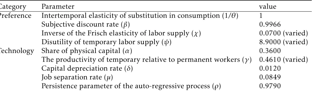
over a long spell.3 Figure 1 illustrates the diff_{erences among three related industry}

cate-gories, and the shaded areas in the figure denote the recessions identified by the NBER. It is

obvious that the three series exhibit a similar growth pattern, even though a persistent gap

between any two of them exists. For example, the number of temporary workers measured

by employment at the industry level, i.e., personnel supply services (SIC-7360), increases at

an annual rate of 8.9 percent during 1972–2000. Despite the existence of slight diff_erences

across industries, temporary workers in general account for about 2-3 percent of the total

non-farm employment in 2000. Nowadays, the share measured by employment by industry

of temporary help services (NAICS-56132) is nearly 2.1 percent.

As displayed in Figure 1, the share of temporary to total workers exhibits a strong

pro-cyclical pattern, and in particular turns into another growing stage after every recession.

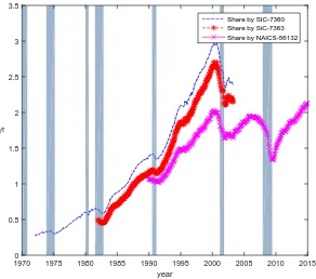
To highlight its periodicity, the bandpass (BP)- and Hodrick-Prescott (HP)-filtered cyclical

components of GDP per capita are also plotted in Figure 2.4 Obviously, the share drops

significantly during the recent episodes of recessions and it attains higher values before the

onsets of subsequent recessions.

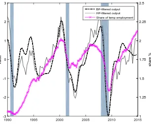
Figure 3 further decomposes aggregate employment into de-trended temporary and

per-manent components. It reveals that temporary employment has a much higher degree of

volatility and higher correlation with output, and permanent employment lags behind in

the cycles.5 As a consequence, the share experiences notable decreases almost

simultane-ously with real GDP per capita during past recessions. One of the possible reasons for this

result is that hiring temporary workers functions as a “buff_{er” device for firms that hesitate}

to adjust their permanent employment level (see Segal and Sullivan, 1997).

Table 1 reports the descriptive statistics of the relevant macro variables and the

re-sults confirm these observations. First, the standard deviation of temporary employment

std(ˆh_t) = 6.66 is higher than that of permanent employmentstd( ˆn_t) = 1.10. Second, the share

3_{The industries that could be used as substitutes for NAISC-56132 (temporary help services) in 1990–2014}

are SIC-7360 (personnel supply services) in 1972-2003 and SIC-7363 (help supply services) in 1982–2003 due to the availability of data. The number of workers in industry SIC-7360 is noticeably greater than that in the others because this broad classification includes sectoral employment agencies.

4_{The coefficient of correlation between the share of temporary employment and de-trended output during}

1990–2014 equals 0.341, whereas the rolling-window correlations display an increasing co-movement pattern between the two variables.

of temporary employment and output are highly correlated and the correlation coeffi_cient

between them is equal to corr(e_t,yˆ_t) = 0.90.Third, the correlation coeffi_{cient between}

tem-porary employment and output corr(ˆh_t,yˆ_t) = 0.91 is higher than that between permanent

employment and output corr( ˆn_t,yˆ_t) = 0.75. Fourth, permanent employment is

character-ized by a lag that is two quarters in length since the value 0.87 is highest for the correlation

coeffi_{cient between permanent employment and (lagged and leading) output in Table 1.}

The complementarity/substitution between temporary and permanent workers can be

examined by observing the wage rates. Based on the annual data provided by Occupational

Employment Statistics, we obtain time series of annual and hourly wages in terms of all

4-digit sub-industries on a national basis. Figure 4 is used to compare the mean wages of

workers in temporary help services and in all industries across occupations. This figure

indicates that a notable wage gap between temporary workers and all the others exists since

the former group is paid roughly 20-30 percent less than the average. In addition, the wage

growth of temporary workers became moderate compared to the average during the Great

Recession and even turned negative during 2001–2002.

In order to explore the cyclical feature of the wage gap between temporary workers and

all the others in detail, we further use data from the National Employment, Hours, and

Earnings database and from the Current Employment Statistics survey. Figure 5 plots the

relative hourly wage of temporary to total non-farm employees. We use wage series from

industries SIC-7323 and NAICS-56132 corresponding to the periods 1982Q1–2003Q1 and

2006Q4–2014Q4 to address the problem of data availability. It should be noted that the

disconnection arises because the two systems have diff_{erent division structures. Figure 5}

presents a similar result to Figure 4 since the two ratios respectively fluctuate between 0.73–

0.83 and 0.66–0.72, hence suggesting a manifest wage gap. Another noteworthy finding

is that the wage ratios reach peaks during periods of the past recessions, and then drop

sharply afterwards. This counter-cyclical behavior justifies our argument that the change

in the relative employment is driven by a TFP shock and the substitution between the two

types of workers plays an important role.

In order to deliver a clear picture, the descriptive statistics and the extent to which our

3 The model

In this section, we build a real business cycles model and derive the conditions that

char-acterize the general equilibrium. The economy that we consider consists of two types of

agents: households and firms. In what follows of this section, we describe the behavior of

each of these agents in turn.

3.1 Households

Assume that the economy is populated by a continuum of identical and infinitely-lived

households, and the population size is normalized to unity for simplicity. The

represen-tative household derives utility from consumption, c_t and incurs disutility from providing

temporary and permanent labor services. In line with Rupert et al. (2000), Chang and Kim

(2006), and Guner et al. (2012a, 2012b), we suppose that the decisions are made by a family

rather than an individual in the household sector. The family consists of two members: one

provides temporary labor services h_t and the other provides permanent labor services h_t.

Accordingly, the preference is modeled specifically by the expected life-time utility

E₀ ∞

∑

t=0 βt

[

c_t1−θ−1

1−θ −ψ

(_n1+χ t 1 +χ +

h1+_t χ

1 +χ

)]

; 1> β >0, θ >0, χ >0, ψ >0, (1)

where E₀ denotes expectations that are conditional on information available at time 0. θ

stands for the inverse of the intertemporal elasticity of substitution in consumption, χ

de-notes the inverse of the Frisch elasticity of labor supply, β represents the household’s

sub-jective discount rate, andψis a parameter that captures the taste for labor supply.

The representative household supplies temporary laborh_t, permanent laborn_t, owns the

capital stockkt, and takes wage rates for temporary and permanent labor,wh,t andwn,t, and

the rental rater_tas given. In addition, the household receives dividend incomed_tby holding

each unit of the firm’s outstanding equity zt at pricept in each period. For simplicity, the

total share of the firm’s outstanding equity is normalized to unity. At each instant in time,

additional equities. The household’s flow budget constraint can be written as:

p_t(z_t+1−z_t) =r_tk_t+w_h,th_t+w_n,tn_t+d_tz_t−c_t−i_t. (2)

Accordingly, the law of motion of the capital stock can be specified as

k_t+1= (1−δ)k_t+i_t; 1> δ >0, (3)

whereδdenotes the rate of capital depreciation.

The representative household’s problem is to choose the sequences{ct, ht, nt, kt+1, zt+1}∞t=0

to maximize the expected life-time utility reported in equation (1), subject to equations (2)

and (3). The first-order conditions that characterize solutions to the optimization problem

are given by:

ψcθ_thχ_t =w_h,t, (4)

(_h t

n_t

)χ

= wh,t

w_n,t, (5)

1 =βE_t

[₍

c_t c_t+1

)θ

(r_t+1+ 1−δ) ]

, (6)

and

p_t=βE_t

[₍

c_t c_t+1

)θ

(p_t+1+d_t+1) ]

. (7)

Equation (4) indicates that the marginal rate of substitution between temporary labor

sup-ply and consumption is equal to the wage rate of temporary labor. Equation (5)

demon-strates that the household’s optimal allocation between temporary and permanent labor

supplies rest on their relative wage rate. Equations (6) and (7) are standard Euler equations

equity.6

3.2 Firms

The production sector is composed of many identical and competitive firms, which can be

treated as a representative firm. Suppose that the firm hires temporary workersh_t, the stock

of permanent workers x_t, and capital services k_t to produce outputy_t. The firm produces

output according to the following CES production function:

y_t=A_tk_tα[x_tσ+ (γh_t)σ]

1−α σ

; 0< γ <1, σ <1, (8)

whereA_trepresents the level of total factor productivity,α denotes the share of capital

ser-vices, and the parameterγ reflects the relative productivity between temporary and

perma-nent labor. The elasticity of substitution betweenh_tandx_tis constant and equal to 1/(1−σ)

with an imperfect substituteσ <1.

In line with Chen and Lai (2015), we assume that in order to accumulate the stock of

permanent workers in period t + 1, the firm needs to hire a flow of new recruits v_t one

period before.7 Accordingly, the law of motion of permanent employment can be written

as:

x_t+1= (1−µ)xt+vt; 0< µ <1, (9)

whereµdenotes an exogenous separation rate.

When the firm hires the new recruits, it then incurs extra labor adjustment costs, which

are considered to be the induced costs from advertising for, screening, and training the new

recruits (see Merz and Yashiv, 2007). The net adjustment costs arising from training the new

6_{It is noteworthy that, by denoting the Lagrange multiplier of the household’s flow budget constraint (2)}

byλt, equation (7) can be rewritten aspt=∑∞j=1βj λ

t+j

λt dt+j, whereβ

j λt+j

λt is the discount rate for periodt+j. As a consequence, this expression implies that the equity price equals the discounted present value of the future dividend income that the household will receive.

7_{Chen and Lai (2015) focus on the case in which only permanent workers are hired in the production}

process and they discuss the relationship between the forward-looking properties of labor demand and news shocks. Diff_{erent from their study, we assume that the firm hires both temporary and permanent workers}

recruits are rationalized and examined by Hamermesh (1995). Here, we adopt this narrow

definition and focus on net hires, namely, the new recruits net of the dismissed permanent

workers. The advantage behind this setting stems from the fact that it not only simplifies

the solution at the steady state but is also consistent with the implication that the dismissed

workers are presumed to be experienced. As a result, there is no need to provide additional

training for them.

On the other hand, the firm accumulates its stock of permanent workers while

fac-ing increasfac-ing adjustment costs, and without loss of generality the costs are modeled as

a quadratic function to depress a rapid adjustment (see, e.g., Blatter et al., 2012; Cooper and

Willis, 2009; Gal´ı and van Rens, 2010; Sargent, 1978). The setting of the adjustment costs is

crucial for generating the observed lagged behavior of permanent employment, as proposed

by Kydland and Prescott (1991), since it diminishes the demand for permanent workers and

in turn the demand for currently new recruits.

Accordingly, the firm’s profits as well as the household’s dividend incomes can be

ex-pressed as:

d_t=y_t−w_n,tn_t−w_h,th_t−r_kk_t−φ

2

(x_t+1−xt)2

x_t ; φ≥0, (10)

where the intensity parameter φ governs the size of the net adjustment costs in terms of

output. The costs are expressed as a quadratic form of the diff_{erence between the stocks of}

permanent workers in periodstandt+ 1.

Equation (9) specifies that new recruits need one period to accumulate experiences and

skills before turning their status into permanent workers in the next period. In fact, we

observe in reality that new recruits may need several periods to complete their training.

The more general scenario is presented below. Let l_i,t denote the new recruits that the firm

employs at time t, and they need i periods to accumulate experiences and skills before

becoming permanent workers. Let b represent the total number of periods required for

each new recruit. Therefore, the aggregate new recruits at timetcan be expressed as:

v_t= b ∑

i=1

The law of motion of the recruits is given by:

l_i,t+1=l_i+1,t; i= 1,2, ..., b−1. (12)

Moreover, the law of motion of permanent employment in equation (9) is modified to

be-come:

x_t+1= (1−µ)x_t+l_1,t; 0< µ <1. (13)

Here we present the general conditions, but in order to discuss the model’s implications, we

will compare cases corresponding to specific valuesb= 0,4 in Section 4.

The objective of the representative firm is to maximize a stream of discounted profits

π_t, which is the sum of the current profits d_t and the discounted value of expected future

profitsDt:

π_t=d_t+D_t=d_t+E_t

[_∑∞

j=1

βjλt+j λ_t dt+j

]

, (14)

whereβj λ_λt+j

t is the discount rate for periodt+j. The firm chooses the sequence{kt, ht, vt, xt+1}

to maximize (14), subject to equations (8), (9), and (10). Let η_t denote the corresponding

Lagrange multiplier. The optimum conditions necessary for the firm with respect to the

indicated variables are:

k_t:r_t=αyt

k_t, (15)

h_t:w_h,t= (1−α) (γht) σ

xσ_t + (γh_t)σ

y_t

h_t, (16)

l_1,t+b−1:Et        1

βb−1_λ

t+b−1

b ∑

a=1

βa−1λ_t+a−1wn,t+a−1

      

=E_t

[

η_t+b−1−φ

(

x_t+b−xt+b−1 x_t+b−1

)]

and

x_t+1:ηt=βEt       

λ_t+1 λ_t      

(1−α)xσ_t+1 x_tσ₊₁+ (γh_t+1)σ

y_t+1

x_t+1−wn,t+1+ φ

2 (

x_t+2−x_t+1 x_t+1

)2

−φ

(

x_t+2−x_t+1 x_t+1

)

+ (1−µ)η_t+1

             . (18)

As indicated in equations (15) and (16), the production inputs k_t and h_t are paid on the

basis of their marginal product. Also note that equation (17) illustrates the firm’s

opti-mal intertemporal choice regarding the new recruits based on its forward-looking decisions

since it takes the current wage, training costs, and the stream of future marginal products

into account.

3.3 The competitive equilibrium

The competitive equilibrium condition is defined as a sequence of allocations{c_t, h_t, n_t, k_t+1, zt+1}

of the representative household and{k_t, h_t, v_t, x_t+1}of the representative firm such that given

the prices {p_t, r_t, w_h,t, w_n,t}, the household maximizes (1) and the representative firm

maxi-mizes (14) and all of the markets are cleared. The market clearing conditions in the equity,

permanent labor, and goods markets are given by

z_t= 1, (19)

n_t=v_t+x_t, (20)

and

c_t+k_t+1−(1−δ)k_t+φ 2

(x_t+1−x_t)2

x_t =Atkt

α[

x_tσ+ (γh_t)σ]

1−α σ

, (21)

Equation (19) implies the equilibrium condition for the equity market given that the

out-standing equity of the economy is normalized to unity. Equation (20) illustrates that the

supply of permanent labor equals the aggregate of new recruits and the workers actually

equa-tion (21) is derived from combining (2), (3), (8), and (9) given (19), in which z_t = 1 for all

t.

Finally, the logarithm of TFP is set to follow a stationary first-order autoregressive

pro-cess,

log(A_t) =ρlog(A_t−1) +εt, (22)

where ρ is the persistence parameter and the technology shock εt is a white noise with

varianceσ_ε2.

4 Main results

Given the model’s complexity, we resort to numerical methods to solve the model by

lin-earizing the dynamic equations around the steady state.8 Let a variable with “∧”denote its

percentage deviation from the stationary value, namely, ˆB_t= (B_t−B)/Bfor any endogenous

variable B_t in our model. We begin by characterizing a benchmark economy, in which the

structural parameters are divided into two groups. Every parameter in the first group is

ei-ther tied to a commonly used value or calibrated to match the US data, and every parameter

in the second group is estimated by using the Simulated Method of Moments (SMM). We

then show how the model produces aggregate variations in response to a shock to TFP given

these parameter values. To better explain the role of each of the main channels, we also

com-pare the model’s responses to diff_{erent structural parameters that bring about implications}

of interest.

4.1 Benchmark parameterization

We first set the capital share α = 0.36 and the intertemporal elasticity of substitution in

consumption 1/θ = 1 (i.e., θ = 1), and the values are selected by those commonly used in

the business cycle literature. In line with Christiano et al. (2008), the subjective discount

8_{A detailed derivation of the stationary values of essential macro variables will be provided in Appendix}

factor β is set equal to 1.01358−0.25, so that it matches the average annual real return on

three-month Treasury bills of 1.36%. Following Cooley and Prescott (1995), we set the

capital depreciation rate δ = 0.012. As for the value of the weight parameter in the utility

function ψ, we set it to match the stationary value of the employment rate (the ratio of

aggregate employment to population), namely,N =n+h= 0.61. As regards the productivity

of temporary workers relative to permanent onesγ, we set it to match the stationary value

of the wage gap between these two kinds of laborw_h/w_n= 0.75.

Moreover, the parameter that governs the intertemporal elasticity of substitution in labor

χ is set to match the stationary value of the temporary to aggregate employment ratio e =

h/N = 0.0165.9 We follow Hall (2005) and set the monthly separation rate at 3.5%, which

corresponds to the quarterly separation rate of permanent laborµ= 1−(1−0.035)3−0.0165 =

0.0849. In addition, we set the total number of periods required for each new recruit to

accumulate the experiences and skills needed to become permanent workers asb= 4, which

is consistent with the value used by Carneiro et al. (2012). Finally, in line with the value

estimated by King and Rebelo (1999), we simply setρ= 0.979. Also note that the calibrated

values of ψ, γ, and χ will vary with respect to diff_{erent SMM estimates of parameters.}10

Panel A of Table 2 reports the values of the calibrated parameters in the first group.

4.2 SMM estimation and the quantitative results

We apply SMM to estimate the set of the remaining parameters in the second group, which

is denoted by a 3×1 vectorΘ_{={σ, φ, σ}2

ε}. The parameters are estimated by minimizing the distance between the empirical moments from the data and the simulated moments based

on our model. Letm stand for the vector of moments computed from real data, andms for

the vector of averaged simulated moments overM= 20 simulations, the same sample size as

for the data. Accordingly, given the sample size of dataT, the estimation of the parameters

9_{The share of temporary employment is set at 1.65% which is the stationary value.} 10_{Given these data moments used for the calibration in the steady state (N = 0.61, w}

h/wn = 0.75, and

will proceed by choosing ˜Θ_{to solve the optimization problem}

˜

Θ_{= arg minJ(}Θ_{) =} T M

1 +M[m−m

s_(Θ)]W[m−ms_(Θ)]′_{, (23)}

where W is a positive-definite weighting matrix, which is computed by the Newey-West

estimator.

The four targeted moments that we select are informative for estimating the SMM

pa-rameters. The reason for choosing these targeted moments to estimate the vector of

param-etersΘ_{={σ, φ, σ}2

ε}can be briefly stated as follows.

First, the standard deviation of the temporary employmentstd(ˆht) is informative in

de-termining the parameter σ, which governs the elasticity of substitution between

tempo-rary and permanent employment.11 Second, the coeffi_{cients of correlation between}

tempo-rary employment and output corr(ˆh_t,yˆ_t) and between permanent employment and output

corr( ˆnt,yˆt) are closely correlated with the intensity parameter of labor adjustment costs φ.

Hence, they provide information about the value ofφ.12 Third, we will show that the

stan-dard deviation of output std( ˆyt) is crucial for determining the variance of the technology

shockσ_ε2. Accordingly, we usestd( ˆy_t) to estimate the variance of the technology shockσ_ε2.

Our data are obtained from the BLS and FRED databases during the period 1990Q1–

2014Q4 in the quarterly frequency, and we thus have the sample size T = 100.13 Panel B

of Table 2 summarizes the SMM estimates of parameters. The targeted and selected

(non-targeted) moments for the US data are reported in Table 3, along with the simulated

mo-11_{A high value ofσ implies a high degree of substitutability between temporary and permanent}

employ-ment. If the value of σ is higher, the firm tends to hire more temporary workers than permanent workers in response to a positive technology shock. This eff_{ect results in an increase in the volatility of temporary}

employment.

12_{If the value ofφis higher, the firm will hire more temporary workers but fewer permanent ones to produce}

in response to the positive technology shock. As a result, this eff_{ect leads to a rise in the correlation between}

temporary employment and output and a reduction in the correlation between permanent employment and output.

13_{There are eight time series variables used for the calibration and SMM estimation, which are Nominal}

ments based on our model. Table 4 displays a summary of the simulated coeffi_{cients of}

correlation between employment and output.

As reported in Panel B of Table 2, the point estimate of the parameterσ is 0.960, which

implies that the elasticity of substitution between permanent and temporary labor equals

25.14 The intensity parameter of labor adjustment costsφ is estimated to be around 9 and

the standard deviation of the technology shock σε is estimated to be 0.802. Since the

chi-square statistic at the 95% level is χ₀2_.05(1) = 3.84, the test statisticJ = 0.30 implies that the

model cannot be rejected by the data.

Tables 3 and 4 confirm that the benchmark model well characterizes the four stylized

facts that we have previously documented. First, temporary employment is more volatile

than permanent employment. Specifically, the model generates the simulated standard

de-viation of temporary employment std(ˆht) = 6.11, which is much higher than that of

perma-nent employmentstd( ˆn_t) = 0.49. Second, the model also generates a strong pro-cyclicality of

the share of temporary employment, which is exhibited by the simulated coeffi_{cient of}

cor-relation between the share of temporary employment and output corr(e_t,yˆ_t) = 0.77. Third,

the coeffi_{cient of correlation between temporary employment and outputcorr(ˆht,yˆt) = 0.81}

is much higher than that between permanent employment and output corr( ˆn_t,yˆ_t) = 0.69.

Fourth, Table 4 shows that our model can generate the two-quarter lagged behavior of

per-manent employment, since the valuecorr( ˆn_t+2,yˆ_t) = 0.82 is the largest in column 8.

4.3 Impulse response analysis

In this subsection, we show how the relevant variables will adjust in response to an

unan-ticipated rise in total factor productivity. Figure 6 depicts their impulse responses to the

technology shock in the benchmark economy. Assume that the economy starts at its

sta-tionary equilibrium in period 0. In period 1, a 1-percent persistent increase in total factor

productivity leads to changes in the relevant macro variables.

First, we restrict our attention to the impulse responses of permanent employment and

aggregate employment. Figure 6 shows that permanent employment is increased

moder-14 _{The value is much larger than the elasticity of substitution estimated by Cappellari et al. (2012), since}

ately upon the arrival of the positive shock at the beginning (in period 1), and then

per-manent employment keeps on rising but at a decreasing rate after period 1. This result

can be explained intuitively as follows. When the positive shock occurs, the firm raises its

expected future profits and in turn increases its demand for permanent workers because

of its forward-looking decisions. Since training permanent workers takes time and incurs

additional adjustment costs, this channel causes the rises in permanent employment to be

lagged and also relatively smooth. In addition, given that permanent employment accounts

for approximately 98% of aggregate employment, it is reasonable for the dynamics of the

aggregate employment to be similar to that for permanent employment.

Second, we examine the impulse response of temporary employment to the positive

shock. As exhibited in Figure 6, temporary employment rises by more than 5% upon the

arrival of the shock and then it continues to decline afterwards. In addition, it is

notewor-thy that in period 1 the increase in temporary employment is considerably larger than that

in the permanent counterpart. Here a question arises because of the result displayed in

Fig-ure 6. Why does the firm tend to hire temporary rather than permanent workers in the short

run in response to the shock? To answer this question, we need to pay special attention to

the following two points. First, the adjustment of permanent workers is time-consuming

since it takes a few periods for the new recruits to accumulate experiences and skills and to

become permanent workers. Second, there exists a high degree of substitutability between

temporary and permanent labor since the estimated elasticity of substitution is at a high

level, i.e., 1/(1−σ) = 25. Based on these two reasons, when the positive shock arrives, the

firm is motivated to hire more temporary workers to substitute for the permanent

counter-parts even though the former ones are less productive. On the other hand, when the time

horizon is getting longer, the firm will accumulate the stock of permanent workers because

their higher productivity is taken into account in the long run. This leads to the decline in

temporary employment after its initial rises.

Third, the last panel in Figure 6 depicts the impulse response of the share of temporary

employment, which is similar to that of temporary employment. Because the share equals

the ratio of temporary employment to aggregate employment, the changes in the share of

employment. Given that permanent employment adjusts slowly, the immediate rise in the

share of temporary employment upon the arrival of the positive shock mostly results from

the increase in temporary employment (over 5%). Thereafter, the share of temporary

em-ployment continues to rise at a decreasing rate. This result is derived from the fact that

temporary employment keeps on rising at a diminishing rate and meanwhile permanent

employment keeps on rising at an increasing rate.

Finally, Figure 6 also indicates that, in response to the increase in TFP, the household

tends to have a higher expected life-time income and this increase stimulates its

consump-tion. Moreover, the rise in aggregate employment in response to the positive shock further

stimulates the investment in physical capital. As a result, this shock leads to persistent rises

in output.

4.4 Implications of applying sensitivity analysis

In this subsection, we would like to intuitively explain why our benchmark model can

suc-cessfully capture the cyclical behavior of temporary and permanent employment in the US

economy. To this end, compared with the benchmark economy, we perform sensitivity

anal-ysis in the following three cases: (i) where there is a low degree of substitution between

temporary and permanent labor (i.e.,σ = 0.01), (ii) in the absence of job training (i.e.,b= 0),

and (iii) in the absence of the labor adjustment cost (i.e., φ = 0). Figures 7-9 respectively

depict the impulse responses of variables{yˆ_t, ˆh_t, ˆn_t,e_t}to a 1-percent persistent increase in

TFP in the three cases, and Table 5 reports the simulated moments in association with these

three cases. For the purpose of comparing the results of the benchmark economy, in each

sensitivity analysis we solely turn off_{one mechanism without re-estimating the parameters.}

More precisely, except for σ in (i), b in (ii), and φ in (iii), the remaining parameters that

we use in doing the sensitivity analysis are the same as those calibrated in Section 4.1 and

estimated in Section 4.2.

In the first case, when we set σ = 0.01, the elasticity of substitution between

tempo-rary and permanent labor 1/(1−σ) is reduced to around unity (compared with σ = 0.960

and e = 25 in the benchmark economy). Figure 7 depicts that, in response to a positive

temporary alternatives as a substitute for permanent workers during the training periods.

Put diff_{erently, given the same wage ratio between the two types of workers, the share of}

temporary employment is consequently decreased compared to the benchmark case (see the

bottom right panel of Figure 7).

The simulated moments in association with the first case (i.e., σ = 0.01) are depicted

in column 4 of Panel A in Table 5, which shows that the following three moments are too

low to match the data: the standard deviation of temporary employmentstd(ˆh_t), the

stan-dard deviation of the share of temporary employmentstd( ˆet), and the correlation coefficient between the share of temporary employment and outputcorr( ˆe_t,yˆ_t). We can explain this

re-sult by focusing on the impulse response displayed in Figure 7. Compared to the benchmark

economy, a loweredσ induces the firm to hire more permanent workers and to lower its

cur-rent demand for temporary ones. This change leads to the reductions in the volatilities of

temporary employment and the share of temporary employment. Moreover, since the

pos-sibility of hiring temporary alternatives as a substitute for permanent workers is reduced,

the decrease inσ leads the share of temporary employment to be less pro-cyclical.

In the second case, we discuss the scenario in which the time-to-build mechanism for job

training is absent, i.e.,b= 0. It should be noted thatb= 0 implies that each new recruit

im-mediately becomes a skilled and trained permanent worker once he is hired. Consequently,

the law of motion of new recruits v_t in equation (11) and the law of motion of the stock

of permanent employment xt in equation (12) are shut down, and the model degenerates

to a standard RBC model.15 In such a case, we show the transitional dynamics of the

rele-vant variables {yˆt,hˆt,nˆt, et}in response to a positive TFP shock in Figure 8. As exhibited in

Figure 8, both permanent and temporary employment rises in response to the positive TFP

shock because now the new recruits can directly participate in production. Compared to the

benchmark case, the absence of the time-to-build mechanism leads to more direct and rapid

responses of the variables ˆyt, ˆht, ˆnt and et to the TFP shock, thereby causing their lagged

behavior to vanish.

15_{In the case of b = 0, the law of motion of new recruitsh}

t (11) and the law of motion of the stock of

permanent employmentxt (12) will degenerate, and the model is reduced to a standard real business cycle

The simulated moments in association with the absence of job training (i.e., b = 0) are

reported in column 5 of Panel A in Table 5. They indicate the nearly perfect positive

corre-lations between output and the variables: temporary employment, permanent employment,

and the share of temporary employment. Moreover, as reported in Panel B in Table 5, in

as-sociation withb= 0, permanent employment is no longer characterized by lagged behavior.

This result can be grasped by referring to Figure 8, i.e., in a standard RBC model, both types

of employment and output display a high synchronization in response to the TFP shock.

We then discuss the third case where labor adjustment costs are absent, i.e.,φ = 0. The

result in Figure 9 reveals that the fluctuations in ˆy_t, ˆh_t, ˆn_t, and e_t are amplified because of

the reduction in labor adjustment costs. The interpretation is straightforward. Since a sharp

increase in permanent workers now becomes less costly, the firm will immediately adjust its

stock of permanent workers by creating more new recruits. Accordingly, the moderate

de-cline in the share of temporary employment during the first four periods is largely explained

by this immediate adjustment. Moreover, the significant increase in ˆyt and falls in ˆht and

e_t at t = 5 are derived from the fact that a number of recruits are becoming permanently

workers.

Finally, the simulated moments in association with the absence of labor adjustment (i.e.,

φ= 0) are reported in column 6 of Panel A in Table 5. In contrast to the smooth adjustment

of permanent employment in the benchmark economy, the absence of labor adjustment costs

leads to increases in the volatility and pro-cyclicality of permanent labor. As a consequence,

the adjustment of permanent labor is more elastic, thereby causing permanent employment

to not lag within the cycle.

4.5 Labor hoarding behavior

Figure 6 also displays how the firm reduces its demand for temporary workers but

main-tains a certain number of skilled and permanent workers during the recession. Since the

firm shrinks its stock of permanent workers only slowly, the labor hoarding eff_{ect leads to}

a moderate variation of output in the short run. Specifically, the calibrated model predicts

that a 1 percent decline in TFP brings about a 3.39-percent decrease in temporary

drops by 1% upon the arrival of the negative shock and the figure is around 50% lower

than the decline in output as the economy reaches another steady state (i.e., -1.5%). This

result suggests that the loss of the stock of permanent workers has a persistent impact on

the output in the long run.

5 Conclusion

The data for the US labor market reveal the following stylized facts involving temporary

workers: (i) a higher volatility of temporary employment than of permanent employment;

(ii) a strong pro-cyclicality of the share of temporary employment; (iii) the lagged behavior

of aggregate employment; and (iv) a stronger correlation between temporary employment

and output than in the case of the permanent counterpart. Given that the standard RBC

model does not draw a distinction between temporary and permanent employment, it is

unable to provide a plausible explanation for these observed facts.

This paper proposes three channels related to distinguishing temporary employment

from permanent employment. The first channel has to do with the substitutability between

temporary and permanent workers. The second channel is concerned with the

time-to-build mechanism for job training, which leads new recruits to become productive

perma-nent workers. The third channel relates to the costs of training permaperma-nent workers. By

incorporating these three channels into into the standard RBC model, this paper finds that

the modified model is able to explain the above stylized facts in the US labor market.

More-over, this paper also finds that the modified model provides a plausible explanation for the

Table 1: Cyclical behavior of temporary and permanent employment in the US economy

Moments

Standard deviation of output std( ˆy_t) 1.10

Standard deviation of share of temporary employment std(et) 0.10

Standard deviation of temporary employment std(ˆht) 6.66

Standard deviation of permanent employment std( ˆn_t) 1.10

Correlation of coeffi_{cient between the share of temporary employment and output corr(et,yˆt) 0.90}

Correlation of coeffi_{cient between temporary employment and output corr(ˆht,yˆt) 0.91}

Correlation of coeffi_{cient between}

permanent employment and 3-period lagged output corr( ˆnt+3,yˆt) 0.81

permanent employment and 2-period lagged output corr( ˆnt+2,yˆt) 0.87

permanent employment and 1-period lagged output corr( ˆn_t+1,yˆ_t) 0.84

permanent employment and output (contemporaneous) corr( ˆnt,yˆt) 0.75

permanent employment and 1-period lead output corr( ˆnt−1,yˆt) 0.56

permanent employment and 2-period lead output corr( ˆn_t−2,yˆt) 0.34

permanent employment and 3-period lead output corr( ˆnt−3,yˆt) 0.12

Note: The sampling period is 1990:Q1−2014:Q4. Except for et, all of the other variables (for ˆyt,hˆt,nˆt) are

Table 2: Parametrization of the benchmark model

Panel A: Calibrated parameters

Category Parameter value

Preference Intertemporal elasticity of substitution in consumption (1/θ) 1

Subjective discount rate (β) 0.9966

Inverse of the Frisch elasticity of labor supply (χ) 0.0700 (varied)

Disutility of temporary labor supply (ψ) 8.9000 (varied)

Technology Share of physical capital (α) 0.3600

The productivity of temporary relative to permanent workers (γ) 0.4610 (varied)

Capital depreciation rate (δ) 0.0120

Job separation rate (µ) 0.0849

Persistence parameter of the auto-regressive process (ρ) 0.9790

Panel B: Estimated parameters by SMM

σ φ σ_ε2 J χ₀2_.05(1)

0.960 8.903 0.673

0.30 3.84

(0.002) (0.561) (0.039)

Table 3: Calibration of the parameters

Moments Data Model

Targeted

std( ˆy_t) 1.10 1.05

std(ˆh_t) 6.66 (6.05) 6.11 (5.82)

corr(ˆh_t,yˆ_t) 0.91 0.81

corr( ˆn_t,yˆ_t) 0.75 0.69

Non-targeted (selected)

std( ˆc_t) 0.79 (0.72) 0.38 (0.35)

std(ˆi_t) 4.15 (3.77) 2.77 (2.64)

std( ˆn_t) 1.10 (1.00) 0.49 (0.47)

std( ˆN_t) 1.17 (1.06) 0.52 (0.50)

std(e_t) 0.10 0.10

corr( ˆNt,yˆt) 0.78 0.81

corr(e_t,yˆ_t) 0.90 0.77

Note: The sampling period is 1990:Q1–2014:Q4. All of the variables (for

gt = ˆNt,hˆt,nˆt, et) are de-trended by the HP-filter and the smoothing parameter

Table 4: Coeffi_{cients of correlation between de-trended output and employment variables}

Source Data Model

Coef. of Corr. Nˆ_t hˆ_t nˆ_t e_t Nˆ_t hˆ_t nˆ_t e_t

corr(g_t+3,yˆ_t) 0.80 0.52 0.81 0.47 0.70 -0.08 0.77 -0.14

corr(g_t+2,yˆ_t) 0.87 0.73 0.87 0.69 0.80 0.16 0.82 0.10

corr(g_t+1,yˆt) 0.86 0.88 0.84 0.85 0.84 0.46 0.80 0.40

corr(g_t,yˆ_t) 0.78 0.91 0.75 0.90 0.81 0.81 0.69 0.77

corr(g_t−1,yˆt) 0.60 0.83 0.56 0.85 0.55 0.60 0.46 0.57

corr(g_t−2,yˆt) 0.38 0.68 0.34 0.72 0.36 0.44 0.29 0.43

corr(g_t−3,yˆt) 0.16 0.48 0.12 0.54 0.22 0.35 0.17 0.34

Note: All the variables are expressed in quarterly frequencies. Then, the HP-filter is applied with respect to all variables to remove the eff_{ects of the trend}

components. Each amount represents the coeffi_{cient of correlation between a}

Table 5: Sensitivity analysis

Panel A: simulated moments

Moments Data Benchmark. σ = 0.01 b= 0 φ= 0

std(ˆh_t) 6.66 6.10 0.78 4.12 6.21

std( ˆn_t) 1.10 0.49 0.82 0.44 1.05

std(e_t) 0.10 0.10 0.01 0.06 0.09

corr(ˆh_t,yˆ_t) 0.91 0.81 0.98 1.00 0.34

corr( ˆn_t,yˆ_t) 0.75 0.69 0.89 1.00 0.87

corr(e_t,yˆ_t) 0.90 0.77 0.08 1.00 0.21

Panel B: Coeffi_{cients of correlation between de-trended output and employment variables}

Source Data Benchmark σ= 0.01 b= 0 φ= 0

Coef. of Corr. hˆ_t nˆ_t hˆ_t nˆ_t hˆ_t nˆ_t hˆ_t nˆ_t hˆ_t nˆ_t

corr(g_t+3,yˆt) 0.52 0.81 -0.08 0.77 0.49 0.51 0.20 0.20 -0.34 0.16

corr(g_t+2,yˆ_t) 0.73 0.87 0.16 0.82 0.58 0.70 0.41 0.41 -0.13 0.36

corr(g_t+1,yˆ_t) 0.88 0.84 0.46 0.80 0.75 0.85 0.67 0.67 0.09 0.59

corr(g_t,yˆ_t) 0.91 0.75 0.81 0.69 0.98 0.89 1.00 1.00 0.34 0.87

corr(g_t−1,yˆt) 0.83 0.56 0.60 0.46 0.75 0.73 0.71 0.71 0.36 0.73

corr(g_t−2,yˆt) 0.68 0.34 0.44 0.29 0.55 0.62 0.47 0.47 0.42 0.65

corr(g_t−3,yˆt) 0.48 0.12 0.35 0.17 0.42 0.54 0.28 0.28 0.50 0.61

year

1970 1975 1980 1985 1990 1995 2000 2005 2010 2015

%

0 0.5 1 1.5 2 2.5 3 3.5

Share by SIC-7360 Share by SiC-7363 Share by NAICS-56132

Figure 1: The share of temporary employment measured by diff_{erent industry classifications}

1990 1995 2000 2005 2010 2015

value

-3 -2 -1 0 1 2 3

BP-filtered output HP-filtered output Share of temp employment

share %

1 1.25 1.5 1.75 2 2.25 2.5

Permanent employment (left) and output (right)

1990 1995 2000 2005 2010 2015

-5 -3 -1 1 3 5

-5 -3 -1 1 3 5

Permanent employment Output

Temporary employment (left) and output (right)

1990 1995 2000 2005 2010 2015

-25 -15 -5 5 15 25

-5 -3 -1 1 3 5

Temporary employment Output

(hourly wage)

year

1995 2000 2005 2010 2015

value

10 12 14 16 18 20 22 24

Temporary Aggregate

(annual wage)

year

1995 2000 2005 2010 2015

value

×104

2 2.5 3 3.5 4 4.5 5

Temporary Aggregate

← SIC-7363

NAICS-56132 →

year

1980 1985 1990 1995 2000 2005 2010 2015

ratio

0.6 0.65 0.7 0.75 0.8 0.85 0.9

Original series Trend component

Trend and random components

2 4 6 8 10 −1.5

−0.5 0.5 1.5

technology (At)

%

2 4 6 8 10 −1.5

−0.5 0.5 1.5

output (yt)

%

2 4 6 8 10 −0.6

−0.3 0 0.3 0.6

consumption (ct)

%

2 4 6 8 10 −4

−2 0 2 4

investment (It)

%

2 4 6 8 10 −6

−3 0 3 6

temporary employment (ht)

%

2 4 6 8 10 −0.8

−0.4 0 0.4 0.8

permanent employment (nt)

%

2 4 6 8 10 −0.8

−0.4 0 0.4 0.8

aggregate employment (Nt)

%

2 4 6 8 10 −0.1

−0.05 0 0.05 0.1

the share of temporary employment (et)

the positive TFP shock

the negative TFP shock

2 4 6 8 10

%

0 0.5 1 1.5

2 output (ˆyt)

σ= 0.96 (benchmark) σ= 0.01

2 4 6 8 10

%

0 2 4 6

8 temporary employment (ˆht)

2 4 6 8 10

%

0 0.25 0.5 0.75

1 permanent employment (ˆnt)

2 4 6 8 10

-0.03 0 0.03 0.06 0.09

0.12the share of temporary employment (et)

2 4 6 8 10

%

0 0.5 1 1.5

2 output (ˆyt)

b= 4 (benchmark) b= 0

2 4 6 8 10

%

0 2 4 6

8 temporary employment (ˆht)

2 4 6 8 10

%

0 0.25 0.5 0.75

1 permanent employment (ˆnt)

2 4 6 8 10

-0.03 0 0.03 0.06 0.09

0.12the share of temporary employment (et)

Figure 8: The impulse responses to an 1% positive TFP shock givenb= 4 (benchmark) and

2 4 6 8 10

%

0 0.5 1 1.5

2 output (ˆyt)

φ= 8.903 (benchmark)

φ= 0

2 4 6 8 10

%

0 2 4 6

8 temporary employment (ˆht)

2 4 6 8 10

%

0 0.25 0.5 0.75 1

1.25 permanent employment (ˆnt)

2 4 6 8 10

-0.03 0 0.03 0.06 0.09

0.12the share of temporary employment (et)

Appendix A

This appendix provides a brief derivation of the equilibrium conditions from the

non-linear form to the non-linearized version in terms of percentage deviations from the steady state.

The competitive equilibrium for the economy is composed of 16 conditions (A1)–(A16).

The endogenous variables are the sequences of quantities {y_t, c_t, h_t, n_t, x_t, v_t, l_1,t, I_t, k_t, z_t, d_t}

and prices{w_h,t, w_n,t, η_t, λ_t, p_t}.GivenA= 1 at the steady state, the stationary relationship at

the competitive equilibrium can be stated as:

z= 1, (A1)

w_h= (1−α)γ σ(_h

x )σ−1

γσ(h x

)σ + 1

1

β −1 +δ

α k

x, (A2)

w_n=w_h(1 +bµ)χ (

h x

)−χ

, (A3)

η = β 1−β

1−βb

βb wn, (A4)

h=         

w_h(h_x)θ

ψ(_kc)θ(k_x)θ

         1

θ+χ

, (A5) γ =       ( h x

)σ−1

w_h w_n

[1−β(1−µ)] (1−βb) + (1−β)βb

(1−β)βb

      −1 σ , (A6) k x =            1

β−1 +δ

αA[γσ(h x

)σ + 1]

1−α σ            1

α−1

, (A7)

c k =

1

β −1 +δ

α −δ, (A8)

y=Akα[

xσ+ (γh)σ]1−_σα

, (A9)

l₁=µx, (A11)

v=bl₁, (A12)

n=x+v, (A13)

d = (1−α)y−w_hh−w_nn, (A14)

p=β(p+d), (A15)

λ=c−θ. (A16)

Let ˆB_t = (B_t −B)/B, where ˆB_t can be any endogenous variable in the model. By

log-linearizing the conditions around B_t’s steady state, we can derive the first-order log-linear

approximations in terms of percentage deviations:

−θcˆ_t= ˆλ_t, (A17)

θcˆ_t+χhˆ_t= ˆw_h,t, (A18)

θcˆt+χnˆt= ˆwn,t, (A19)

0 = ˆλ_t+1−λˆt+βα

y k

( ˆ

y_t+1−kˆt+1

)

, (A20)

ˆ

p_t= ˆλ_t+1−λˆt+β (

ˆ

p_t+1+ d pdˆt+1

)

, (A21)

ˆ

k_t+1= (1−δ) ˆkt+δIˆt, (A22)

nnˆ_t=xxˆ_t+vvˆ_t, (A23)

ˆ

w_h,t= (σ−1) ˆh_t+ ˆy_t−σ(γh)

σ_hˆ

t+xσxˆt

(γh)σ+xσ , (A24)

ˆ

v_t=1

b

b ∑

a=1

ˆ

l1,t+a−1, (A25)

−λˆt+b−1+

1

βb−1 w_n

η

b ∑

a=1

βa−1(λˆ_t+a−1+ ˆwn,t+a−1

)

= ˆη_t+b−1− φµ

η

(_ˆ

l1,t+b−1−xˆt+b−1

)

ˆ

η_t= ˆλ_t+1−λˆ_t+β

η

{

(1−α)xσ−1y

(γh)σ+xσ [

(σ−1) ˆx_t+1+ ˆy_t+1−σ(γh)

σ_hˆ

t+1+xσxˆt+1

(γh)σ+xσ

]}

+β

η

[

−w_nwˆ_n,t+1−φµ(lˆ_1,t+1−xˆ_t+1)+ (1−µ)ηηˆ_t+1], (A27)

ˆ

xt+1= (1−µ) ˆxt+µlˆ1,t, (A28)

ddˆ_t= (1−α)yyˆ_t−w_hh(wˆ_h,t+ ˆh_t)−w_nn(_ˆ

w_n,t+ ˆn_t)

, (A29)

ˆ

y_t= ˆA_t+αkˆ_t+ (1−α)(γh) σ_hˆ

t+xσxˆt

(γh)σ+xσ , (A30)

ˆ

z_t= 0, (A31)

Reference

1. Acemoglu, Daron and J¨orn-Steff_{en Pischke (1999). “Beyond Becker: Training in}

Im-perfect Labour Markets.” Economic Journal,109 (453), F112–F142.

2. Arulampalam, Wiji, Alison L. Booth and Mark L. Bryan (2004). “Training in Europe.”

Journal of the European Economic Association,2 (2–3), 346–360.

3. Autor, David H. (2001). “Why Do Temporary Help Firms Provide Free General Skills

Training?” Quarterly Journal of Economics,116 (4), 1409–1448.

4. Barnichon, Regis (2010). “Productivity and Unemployment over the Business Cycle.”

Journal of Monetary Economics,57 (8), 1013–1025.

5. Berton, Fabio and P. Garibaldi (2012). “Workers and Firms Sorting into Temporary

Jobs.” Economic Journal,122 (562), F125–F154.

6. Blatter, Marc, Samuel M ¨uhlemann and Samuel Schenker (2012). “The Costs of Hiring

Skilled Workers.” European Economic Review,56 (1), 20–35.

7. Booth, Alison L, Juan J. Dolado and Jeff _{Frank (2002). “Symposium on Temporary}

Work: Introduction.” Economic Journal,112 (480), F181–F188.

8. Burnside, Craig, Martin Eichenbaum and Sergio Rebelo (1993). “Labor Hoarding and

the Business Cycle.” Journal of Political Economy,101 (2), 245–273.

9. Cahuc, Pierre, Olivier Charlot and Franck Malherbet (2012). “Explaining the Spread

of Temporary Jobs and its Impact on Labor Turnover.” IZA Discussion Papers No.

6365.

10. Cappellari, Lorenzo, Carlo Dell’Aringa and Marco Leonardi (2012). “Temporary

Em-ployment, Job Flows and Productivity: A Tale of Two Reforms.” Economic Journal, 122

(562), F188–F215.

11. Carneiro, Anabela, Paulo Guimar˜aes and Pedro Portugal (2012). “Real Wages and the

Business Cycle: Accounting for Worker, Firm, and Job Title Heterogeneity.” American