Estimating Egypt’s Potential Output: A Production Function Approach

(1)

Munich Personal RePEc Archive

Estimating Egypt’s Potential Output: A

Production Function Approach

El-Baz, Osama

Economist, [email protected]

20 May 2016

Online at https://mpra.ub.uni-muenchen.de/71652/

(2)

Estimating Egypt

’s Potential Output:

A Production Function Approach

Osama El-Baz

Abstract

The Egyptian economy has witnessed deterioration in its main macroeconomic indicators over the period (2008-2014). The main purpose of the paper was to estimate Egypt's potential output and identify the factors that might be responsible for the divergence of actual and potential output from each other. We used the production function approach to derive estimates of potential output and output gap over the period (1990-2014). The results of the analysis revealed that capital stock was the dominant factor contributing to GDP growth in Egypt, while the share of both labor and total factor productivity in GDP growth rate has been fluctuating over time. Intellectual property protection, efficiency of legal framework in settling disputes, strength of investor protection, and other factors exhibited a strong positive relationship with output gap in Egypt over the period (2010-2014).

1.

Introduction

Potential output is defined as the level of output or productive capacity

that an economy can reach without triggering either upside or downside

pressures on inflation under full employment. The output gap is an

important concept which refers to as the difference between the actual

and potential output in percent of potential output (Blagrave et al. 2015).

When the output gap is zero, it means that there is no either upward or

downward pressure on inflation, as actual demand coincides with

(3)

positive, it means that actual output level "demand" exceeds the potential

level and this would build upside inflation pressures.

Output gap and potential output estimates are important for policymakers

and Economists as it shades light on the economic performance of the

country; as it indicates the relative deviation of actual output from its

potential level and the availability of spare capacity in the economy.

Also, it is an indicator regarding the success of government economic

policies in stimulating economic activity and adopting a business friendly

environment.

This paper consists of seven sections as follows: First: Introduction.

Second: The Egyptian Economy: Challenges and Stylized Facts. Third:

Empirical Methodologies to Estimate Potential Output. Fourth:

Econometric Analysis: The Production Function Approach. Fifth:

Contributions to Potential GDP Growth Rates in Egypt. Sixth: Factors

Affecting Egypt's Output Gap. Seventh: Conclusion and policy

implications.

2.

The Egyptian Economy: Challenges and Stylized

Facts

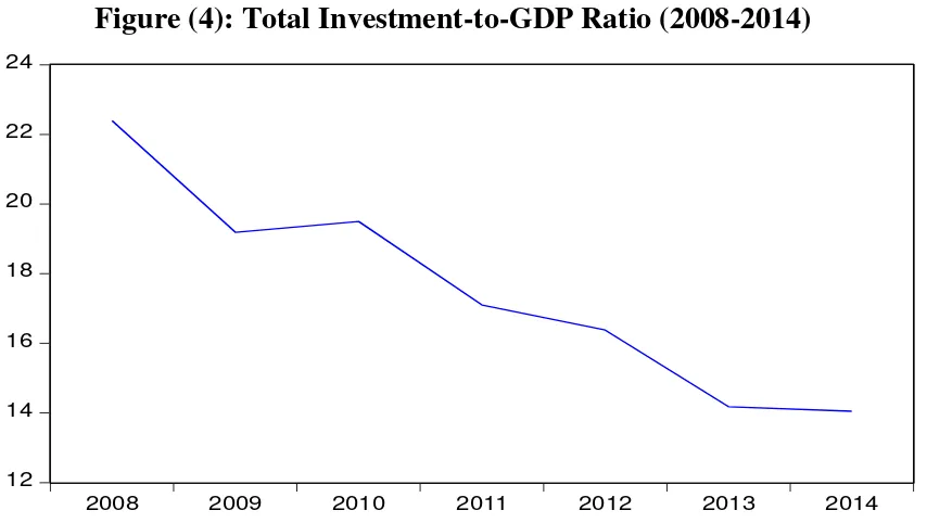
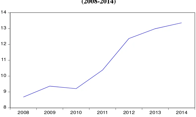
The Egyptian economy has witnessed deterioration in its main

macroeconomic indicators over the period (2008-2014). Real GDP

growth rates over this period recorded an average of about 3.6 percent,

while growth rates exhibited a significant fall starting from 2011 as the

average real GDP growth rate during (2008-2010) was around 5.7 percent

(Figure 1), also real GDP per capita declined after 2011(Figure 2). Both

(4)

after 2011 and recoded around 13.2 percent and 14 percent in 2014,

respectively (Figures 3 & 4). In tandem with a significant increase in

structural budget deficit-to- potential GDP ratio, which increased from

8.3 percent in 2010 to 13 percent in 2014 (Figure 5). Unemployment rate

has also increased from 8.3 percent in 2010 to 13 percent in 2014. To sum

up, the Egyptian economy suffers problems in its macroeconomic

fundamentals and structural reforms needs to be undertaken to put the

economy on a sustainable growth path.

Figure (1): Real GDP Growth Rates (2008-2014)

Source: International Monetary Fund. World Economic Outlook.

Figure (2): Real GDP Per Capita (1000 LE) (2008-2014)

1 2 3 4 5 6 7 8

2008 2009 2010 2011 2012 2013 2014

18.2 18.4 18.6 18.8 19.0 19.2 19.4

[image:4.595.103.494.278.485.2] [image:4.595.99.500.534.744.2]

(5)

Figure (3): National Saving-to- GDP Ratio (2008-2014)

Figure (4): Total Investment-to-GDP Ratio (2008-2014)

10 12 14 16 18 20 22 24

2008 2009 2010 2011 2012 2013 2014

12 14 16 18 20 22 24

[image:5.595.92.510.106.357.2] [image:5.595.89.516.424.665.2]

(6)

Figure (5): Structural Government Budget Balance-to-potential GDP Ratio (2008-2014)

Figure (6): Unemployment Rate in the Egyptian Economy

(2008-2014)

-14 -13 -12 -11 -10 -9 -8 -7 -6

2008 2009 2010 2011 2012 2013 2014

8 9 10 11 12 13 14

[image:6.595.92.499.116.336.2] [image:6.595.100.496.437.674.2]

(7)

3.

Empirical Methodologies to Estimate Potential

Output

All commonly used methodologies to estimate the potential output

involve filtering of the macroeconomic time series to extract the

unobservable underlying potential output level from cyclical variations in

the output series. There are three main methodologies which are

commonly used to estimate potential output, which are singlevariate,

multivariate, and hybrid methods.



Singlevariate Statistical Methods:

Hodrick Prescott (HP) filter has become the most commonly used

statistical method to estimate potential output due to its flexibility in

tracking the fluctuations of trend output and decomposing the aggregate

output into both trend and cyclical components. The HP filter estimates

potential output by minimizing the sum, over the sample period, of

squared distances between actual and potential output at each point in

time, subject to a restriction on the variation of potential output. The

restriction parameter λ captures the importance of cyclical shocks to

output relative to trend output shocks, and thereby controls the

smoothness of the series of potential output; a smaller value of λ indicates a smaller weight of cyclical shocks and leads to a more volatile series of

potential output.

The singlevariate (SV) methods provide an easy tool to estimate potential

output. However, these methods are purely statistical techniques, which

filter the actual GDP data to extract the trend component as its estimate of

potential output. The most common SV filter is the Hodrick-Prescott

(8)

series (output). However, the HP filter does not take into consideration

the information available from other economic indicators such as

inflation or labor market indicators, to guide its estimate of potential

output.



Hybrid Methods:

The Production Function (PF) approach is better than a SV filter

because it allows for more detailed examination of the drivers of potential

output. A downside of this approach is that it assumes capital is always at

its potential. The hybrid approach also suffers from the end of-sample

problems. This approach takes into consideration the contribution of

labor, capital, and total factor productivity to potential output. This

approach will be used in this paper to estimate Egypt's potential output.



Multivariate Methods:

Multivariate (MV) filtering methodologies are used in the literature to

estimate potential output. Some examples are models of Laxton and

Tetlow (1992), Kuttner (1994), Benes and others (2010), Fleischman and

Roberts (2011), and Blagrave and others (2015). MV filtering involves

separating potential output from cyclical fluctuations, through the use of

data and relationships between output and other macroeconomic

variables, such as inflation, labor market indicators, capital formation

indicators, etc. This approach adds economic structure to estimates by

conditioning them on some basic theoretical relationships, such as the

Phillip’s curve equation which expresses the relationship between inflation and output gap. MV filtering methodologies are more

complicated than SV filtering methodologies and require more data, but

are at the same time more reliable because they use more information

(9)

The MV filtering approach needs a long time series data. However it

provides the advantage of imposing well-known empirical relationships.

4.

Econometric Analysis

The Production Function Approach



Methodology:

Following a standard application in the literature (Konuki. 2008) and

(Epstein and Macchiarelli. 2010).the Egyptian economy is assumed to be

characterized by a Cobb-Douglas production function with constant

returns to scale (CRS) (α+β =1).

Y

t

= A

t

L

tα

K

t β

(1)

where Y t is output and Lt, Kt and

A

t are labor and capital, and total

factor productivity (TFP), respectively; and the output elasticities sum up

to one under the assumption of constant returns to scale (CRS).

The Terms on the right hand side of equation (1) are defined as follows:  The labor input: it is defined as the number of people employed

in the economy.

 The capital stock: this series is constructed from total investment assuming perpetual inventories, hence:

K

t

= K

t-1

(1-µ)+ I

t

(2)

capital stock in each period is estimated using the previous-period

stock (net of depreciation) augmented with new investment flows.

Consistent with previous studies, the depreciation rate (

µ)

ranges

(10)

stock an initial value is needed for a reference year, which could be

estimated by the following formula:

K

t

= K

t

/ (µ + i) (3)

Where (i) is the average growth rate of investment over the sample

period included in the analysis.

 The total factor productivity term is obtained from equation (1) as a Solow residual as expressed by equations (4) and (5).

A

t

= Y

t

/ (L

tα

K

tβ

), where:

α= 1

-

β

(4)

Ln At= Ln Yt – (

1-

β

) Ln L

t

–

β Ln K

t

(5)

 Output elasticities to inputs of labor and capital are needed to estimate total factor productivity (TFP), we will estimate them

using the following OLS regression models:

Ln Yt= Ln At +

(1-

β

) Ln L

t

+

β Ln K

t (6)

(LnYt – Ln Lt)= Ln At

+β (Ln K

_t-

Ln L

t) (7)

Equation (7) could be estimated by an OLS regression model to

estimate

β

and

α

, where

(α= 1

-

β

).

 Potential Values of K, A, and L: potential values of capital, labor, and total factor productivity are needed in order to estimate

potential output using the following equation:

Y

* t

= A

*

t

L

*

tα

K

t β

(8)

As for the potential utilization of the capital stock, a capacity

utilization series is not available. In this regard, and consistent with

(11)

capital. Such a simplification mostly relies on the assumption that,

given the perpetual inventories rule, the capital stock can be

regarded as an indicator for the overall capacity of the economy.

Potential values of both total factor productivity and labor could be

estimated by Hodrick Prescott (HP) filter to derive their trend

components from their actual values.



Data and Variables:

o _{Real GDP (Real Output)}_{: real gross domestic product was}

estimated using data for gross domestic product at market prices

deflated by the GDP deflator.

o _{Employed People (Labor):}_{employed people in millions.}

o _{Real Investment:}_{total investment was deflated by the GDP}

deflator.

All data used are from the IMF World Economic Outlook database and

covering the period (1990-2014).



Model Estimation:

o _{The elasticities of output to labor and capital inputs could be}

estimated using the following regression model:

(LnYt

–

Ln Lt)= Ln At

+β (Ln K

t

–

Ln L

t

) (1)

Both the dependent and the explanatory variables were tested

for stationarity using Augmented Dickey Fuller (ADF) unit root

test, they were found to be integrated of order one (Table 1).

The output of the regression model is summarized by (Table 2),

and diagnostic tests were used and it was found that the model

does not suffer any serial correlation, hetroscedsaticity, and

(12)

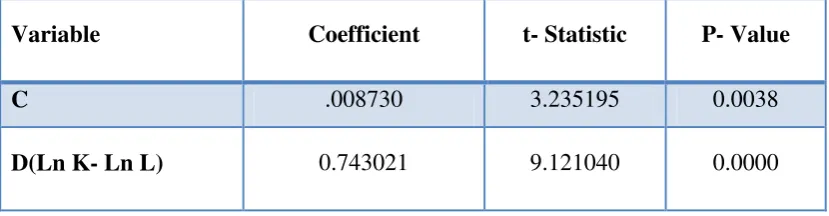
diagnostic tests are in the appendix. The elasticities of output to

capital and labor inputs were found to equal 0.74 and 0.26,

respectively.

Table (1): ADF Unit Root Test for Variables of Equation (1)

Variable t-Statistic P- Value Order of Integration

(LnY – Ln L) -4.241 .0174 I(1)

(Ln K- Ln L) -3.60 .0569 I(1)

Source: Researcher's calculations

Table (2): Elasticity of Output to Capital and Labor Inputs

Variable Coefficient t- Statistic P- Value

C .008730 3.235195 0.0038

D(Ln K- Ln L) 0.743021 9.121040 0.0000

Table (3): Results of Diagnostic Tests

Variable Test Statistic P- Value

Jarque Bera Test of Normality 0.2715 0.8730

Breusch-Godfrey Serial

Correlation LM Test 2.167666 0.1406

Heteroskedasticity Test:

Breusch-Pagan-Godfrey 3.143538 0.0901

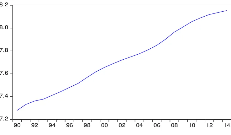
[image:12.595.89.510.205.319.2] [image:12.595.91.506.408.516.2] [image:12.595.91.508.579.753.2]

(13)

o _{Capital Stock was estimated according to equations (2 &3)}

(Figure 7), and total factor productivity was calculated as a solow residual using the following equation (Figure 8):

Ln A

t

= Ln Y

t

–

(1-

β

) Ln L

t

–

β Ln K

t

(2)

Figure (7): The Natural Logarithm of Estimated Capital Stock

(1990-2014)

Figure (8): The Natural Logarithm of Estimated Total Factor

Productivity (1990-2014)

7.2 7.4 7.6 7.8 8.0 8.2

90 92 94 96 98 00 02 04 06 08 10 12 14

.25 .30 .35 .40 .45 .50 .55

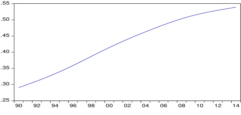
[image:13.595.113.482.247.462.2] [image:13.595.117.478.550.751.2]

(14)

o _{In order to estimate potential output level (Y*), the potential}

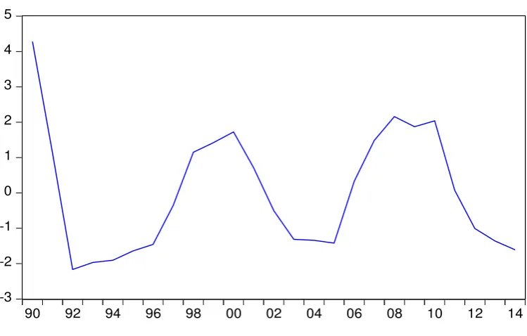
levels of both labor employed (L*) and total factor productivity (A*) were derived as the Hodrick Prescott filtered series of the aggregate series of actual labor and TFP (Figures 9&10). Potential output was estimated using the production function approach (Y*) and was compared to potential output level estimated by the HP filter (YHP*) (Figure 11). Output gap was also estimated, it is important to mention that the Egyptian economy exhibited negative output gaps starting from 2012 (Figure 12).

Figure (9): The Natural Logarithm of Potential Employment

(1990-2014)

Figure (10): The Natural Logarithm of Potential Total Factor Productivity (1990-2014)

2.6 2.7 2.8 2.9 3.0 3.1 3.2 3.3

90 92 94 96 98 00 02 04 06 08 10 12 14

.25 .30 .35 .40 .45 .50 .55

[image:14.595.106.490.319.501.2] [image:14.595.103.492.554.739.2]

(15)

Figure (11): Potential Output Estimates for the Egyptian Economy (1990-2014)

Figure (12): Output Gap Estimates for the Egyptian Economy

(1990-2014)

6.2 6.4 6.6 6.8 7.0 7.2 7.4 7.6

90 92 94 96 98 00 02 04 06 08 10 12 14

Y* YHP*

-3 -2 -1 0 1 2 3 4 5

[image:15.595.98.500.118.369.2] [image:15.595.111.486.488.727.2]

(16)

5.

Contributions to Potential GDP Growth Rates in

Egypt

The production function framework enables us to estimate the

contribution of each factor of production to potential GDP growth.

Changes in these contributions can be assessed as a signal for structural

changes in the economy. The contributions of labor and capital inputs to

potential GDP growth rate were estimated, accounting for their respective

shares in output. Contributions are computed as year-on-year percentage

changes (Epstein and Macchiarelli, 2010). Labor, capital and TFP

contributions sum up to potential GDP growth rates, as according to

equation (1) it is accepted that the sum of percentage changes in labor,

capital , and total factor productivity equals the percentage change in

output "GDP Growth".

The contributions of Labor, capital and TFP to potential GDP growth

rates were estimated (Figure 13). It could be easily visualized that capital

stock was the dominant factor contributing to GDP growth in Egypt over

the period (1991-2014), while the share of both labor and total factor

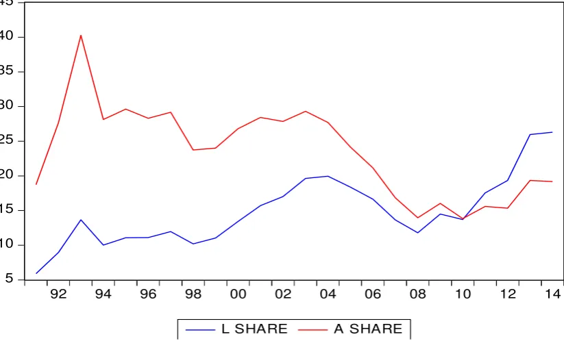
productivity in GDP growth rate has been fluctuating over time. As for

labor and TFP, it is noticed that the relative importance of both of them in

GDP potential growth rate has changed over the period (1991-2014); the

contribution of TFP to potential GDP growth rate over the period

(1991-2010) has been outweighing that of labor, while starting from 2011 the

contribution of labor to potential GDP growth rate exceeded that of TFP

(Figure 14). The average share of labor and TFP in potential GDP growth

rate over the period (2011-2014) recorded 22.3% and 17.4%,

(17)

Figure (13): Contributions to Potential GDP Growth Rates in Egypt (1991-2014)

Source: Researcher's calculation

Figure (14): The Relative Share of Labor and TFP's Contributions to Potential GDP Growth Rates in Egypt (1991-2014)

0 1 2 3 4 5 6 7

92 94 96 98 00 02 04 06 08 10 12 14

L Share K Share A Share

5 10 15 20 25 30 35 40 45

92 94 96 98 00 02 04 06 08 10 12 14

[image:17.595.92.507.120.366.2] [image:17.595.94.506.474.723.2]

(18)

6.

Factors Affecting Egypt's Output Gap

In order to identify the economic factors that might affect output gap in

the Egyptian economy, we will depend on selected sub indices which

falls under the umbrella of the Global Competitiveness Index, and Egypt's

rankings in them were used to identify their relationship with output gap.

The indices used were intellectual property protection, efficiency of legal

framework in settling disputes, strength of investor protection, quality of

overall infrastructure, government budget balance-to-GDP ratio, quality

of the education system, intensity of local competition, pay and

productivity in labor market, availability of financial services and

capacity for innovation.

Data used for these indices are covering the period (2010-2014), and

output gap estimates for the same period were derived from the

production function analysis conducted in section four. It could be

visualized that the rankings of Egypt in all the variables mentioned

earlier are inversely related to output gap; which means that better

rankings of the Egyptian economy in these sub indices implies the

convergence of actual output to potential output or exceeding it with the

(19)

Figure (15): Relationship between Intellectual Property Protection and Output

Gap (2010-2014)

Source: Researchers' Calculations.

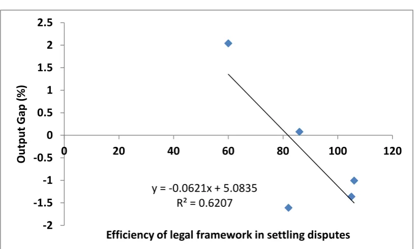
Figure (16): Relationship between Efficiency of Legal Framework in Settling Disputes and Output Gap (2010-2014)

y = -0.0941x + 8.5658 R² = 0.7567 -2

-1.5 -1 -0.5 0 0.5 1 1.5 2 2.5

0 20 40 60 80 100 120

O

u

tp

u

t

Gap

(%)

Intellectual property protection

y = -0.0621x + 5.0835 R² = 0.6207

-2 -1.5 -1 -0.5 0 0.5 1 1.5 2 2.5

0 20 40 60 80 100 120

O

u

tp

u

t

Gap

(%)

[image:19.595.92.500.123.337.2] [image:19.595.91.501.432.677.2]

(20)

Figure (17): Relationship between Strength of Investor Protection and Output Gap (2010-2014)

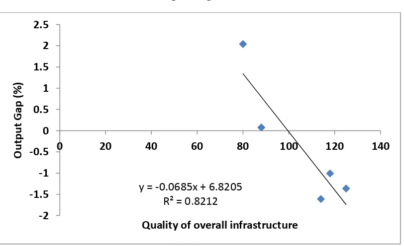
Figure (18): Relationship between Quality of Overall Infrastructure

and Output Gap (2010-2014)

y = -0.0445x + 3.5848 R² = 0.5773

-2 -1.5 -1 -0.5 0 0.5 1 1.5 2 2.5

0 20 40 60 80 100 120 140

O

u

tp

u

t

Gap

(%)

Strength of investor protection

y = -0.0685x + 6.8205 R² = 0.8212

-2 -1.5 -1 -0.5 0 0.5 1 1.5 2 2.5

0 20 40 60 80 100 120 140

O

u

tp

u

t

Gap

(%)

[image:20.595.93.501.108.359.2] [image:20.595.94.500.457.705.2]

(21)

Figure (19): Relationship between Government budget balance/GDP (%)

Figure (20): Relationship between Quality of the Education System

y = -0.211x + 29.204 R² = 0.5418

-2 -1.5 -1 -0.5 0 0.5 1 1.5 2 2.5

130 132 134 136 138 140 142 144 146 148

O

u

tp

u

t

Gap

(%)

Government budget balance/GDP (%)

y = -0.2924x + 40.502 R² = 0.5051 -2.5

-2 -1.5 -1 -0.5 0 0.5 1 1.5 2 2.5

134 136 138 140 142 144 146

O

u

tp

u

t

Gap

(%)

[image:21.595.93.497.115.370.2] [image:21.595.90.503.470.706.2]

(22)

Figure (21): Relationship between Intensity of Local Competition

Figure (22): Relationship between Pay and Productivity

y = -0.1785x + 22.014 R² = 0.8745 -2

-1.5 -1 -0.5 0 0.5 1 1.5 2 2.5

110 115 120 125 130 135

O

u

tp

u

t

Gap

(%)

Intensity of local competition

y = -0.0949x + 10.937 R² = 0.9214

-2 -1.5 -1 -0.5 0 0.5 1 1.5 2 2.5

0 20 40 60 80 100 120 140

O

u

tp

u

t

Gap

(%)

[image:22.595.95.503.134.376.2] [image:22.595.97.500.459.722.2]

(23)

Figure (23): Relationship between Availability of Financial Services

and Output Gap (2010-2014)

Figure (24): Relationship between Capacity for Innovation

y = -0.06x + 6.0735 R² = 0.8614

-2 -1.5 -1 -0.5 0 0.5 1 1.5 2 2.5

0 20 40 60 80 100 120 140

O

u

tp

u

t

Gap

(%)

Availability of financial services

y = -0.0494x + 4.9583 R² = 0.7165

-2 -1.5 -1 -0.5 0 0.5 1 1.5 2 2.5

0 20 40 60 80 100 120 140

O

u

tp

u

t

Gap

(%)

[image:23.595.92.503.136.387.2] [image:23.595.90.504.474.707.2]

(24)

According to the global competitiveness report (2015/2016), the factors

adversely affecting doing business in Egypt include policy instability,

inefficient government bureaucracy, poor work ethics in labor force,

inadequately educated work force, access to finance, inadequate supply of

infrastructure, foreign currency regulations, government instability,

inflation, and other factors (Figure 25).

Figure (25): Factors Negatively Affecting Doing Business in Egypt

Source: World Economic Forum. "Global Competitiveness Report: (2015-2016)".

7.

Conclusion

The Egyptian economy has witnessed deterioration in its main

macroeconomic indicators over the period (2008-2014), including real

GDP growth rate, GDP per capita, saving-to-GDP ratio,

investment-to-GDP ratio, unemployment rate and structural government budget

balances. Under these conditions, it is crucial to stimulate investment in

order to allow actual output to converge to its potential level and avoid

the existence of spare capacity in the economy. 1

1.5 3.2

3.9 4.1

4.4 4.5 5

6.1 7

7.2 9.2

10.1 10.4

10.5 11.8

0 2 4 6 8 10 12 14

Poor Public Health Insufficient Capacity to Innovate Tax Rates Complexity of Tax Regulations Corruption Restrictive Labor Regulations Crime and Theft Inflation Government Instability Foreign Currency Regulations Inadequate Supply of Infrastructure Access to Finance Inadequately Educated Work Force Poor Work Ethics in Labor Force Inefficient Government Bureaucracy Policy Instability

[image:24.595.90.507.240.527.2]

(25)

The main purpose of the paper was to estimate Egypt's potential output

and identify the relationship between selected economic variables and the

estimated output gap, trying to identify the factors that might be

responsible for the existence of negative output gaps witnessed in Egypt

starting from 2012.

The paper shaded light on different methodologies used in the literature

to estimate potential output, and focused on the production function

approach which was used to estimate potential output. The contributions

of labor, capital stock and total factor productivity to potential GDP

growth rates in Egypt over the period (1991-2014) were calculated.

Output gap estimates were also derived and used to visualize their

relationship with selected economic indicators.

The results of the analysis revealed that capital stock was the dominant

factor contributing to GDP growth in Egypt over the period (1991-2014),

while the share of both labor and total factor productivity in GDP growth

rate has been fluctuating over time. The relative importance of labor and

TFP in contributing to GDP potential growth rate has changed over the

period (1991-2014); the contribution of TFP to potential GDP growth rate

over the period (1991-2010) has been outweighing that of labor, while

starting from 2011 the contribution of labor to potential GDP growth rate

exceeded that of TFP.

Intellectual property protection, efficiency of legal framework in settling

disputes, strength of investor protection, quality of overall infrastructure,

government budget balance-to-GDP ratio, quality of the education

system, intensity of local competition, pay and productivity in labor

(26)

exhibited a strong positive relationship with output gap in Egypt over the

period (2010-2014).

It is important for the Egyptian government to exert efforts to promote

investment and facilitate doing business to allow actual output to

approach its potential levels. It is important to promote intellectual

property protection, improve the efficiency of the legal system in settling

disputes, improve the quality of overall infrastructure with more

government expenditure on infrastructural projects, ensuring fiscal

consolidation and low structural budget deficits, improving the quality of

the education system with policies targeting the education- occupation

mismatch problem, ensuring competition in the domestic market and

curbing monopoly practices, improving the skills of the labor force in

order to improve the link between wages and productivity levels,

promoting capital market development to attract foreign direct investment

(27)

References

Epstein,N. and Macchiarelli, C.,2010, "Estimating Poland’s Potential Output: A Production Function Approach". IMF Working Paper No.10/15.

KonukiT., 2008, "ESTIMATING POTENTIAL OUTPUT AND THE OUTPUT GAP IN SLOVAKIA ". IMF Working Paper No. 8/275.

Blagrave, b., R. Garcia-Saltos, D. Laxton, and F. Zhang, 2015, " A Simple Multivariate Filter for Estimating Potential Output". IMF Working Paper No. 15/79.

Laxton, D., and R. Tetlow, 1992, “A Simple Multivariate Filter for the

Measurement of Potential Output,” Technical Report no. 59 (Ottawa: Bank of

Canada).

Kuttner, K. N., 1994, “Estimating Potential Output as a Latent Variable”

Journal of Business and Economic Statistics, Vol. 12, pp. 361–68.

(28)

Appendix

ADF test for (Ln K- Ln L):

Null Hypothesis: LN_K__LN_L has a unit root Exogenous: Constant, Linear Trend

Lag Length: 5 (Automatic - based on SIC, maxlag=5)

t-Statistic Prob.*

Augmented Dickey-Fuller test statistic -3.364543

0.0862

Test critical values: 1% level -4.532598 5% level -3.673616 10% level -3.277364

*MacKinnon (1996) one-sided p-values.

Warning: Probabilities and critical values calculated for 20 observations and may not be accurate for a sample size of 19

Augmented Dickey-Fuller Test Equation Dependent Variable: D(LN_K__LN_L)

Method: Least Squares Date: 05/18/16 Time: 17:09 Sample (adjusted): 1996 2014 Included observations: 19 after adjustments

Variable Coefficient Std. Error t-Statistic Prob. LN_K__LN_L(-1) -1.113173 0.330854 -3.364543 0.0063 D(LN_K__LN_L(-1)) 0.664965 0.252684 2.631609 0.0233 D(LN_K__LN_L(-2)) 0.509315 0.239396 2.127501 0.0568 D(LN_K__LN_L(-3)) 0.621437 0.270473 2.297592 0.0422 D(LN_K__LN_L(-4)) 0.339400 0.207679 1.634253 0.1305 D(LN_K__LN_L(-5)) -0.360083 0.161029 -2.236134 0.0470 C 5.187647 1.530806 3.388833 0.0060 @TREND(1990) 0.010417 0.003507 2.970479 0.0127 R-squared 0.709832

Mean dependent var 0.010094

Adjusted R-squared 0.525179

S.D. dependent var 0.024385

S.E. of regression 0.016803

Akaike info criterion

-5.038943

(29)

ADF test for the first differenced series of (Ln K- Ln L):

Null Hypothesis: D(LN_K__LN_L) has a unit root Exogenous: Constant, Linear Trend Lag Length: 4 (Automatic - based on SIC, maxlag=5)

t-Statistic Prob.*

0.0569

Augmented Dickey-Fuller Test Equation Dependent Variable: D(LN_K__LN_L,2) Method: Least Squares Date: 05/18/16 Time: 17:10 Sample (adjusted): 1996 2014 Included observations: 19 after adjustments

Variable Coefficient Std. Error t-Statistic Prob. D(LN_K__LN_L(-1)) -1.731597 0.480829 -3.601270 0.0036 D(LN_K__LN_L(-1),2) 0.776825 0.395853 1.962406 0.0733 D(LN_K__LN_L(-2),2) 0.709977 0.354013 2.005512 0.0680 D(LN_K__LN_L(-3),2) 0.634470 0.257250 2.466351 0.0297 D(LN_K__LN_L(-4),2) 0.504041 0.211721 2.380689 0.0347 C 0.037389 0.018635 2.006435 0.0679 @TREND(1990) -0.001074 0.001085 -0.990036 0.3417 R-squared 0.637934

Mean dependent var -0.000580

Akaike info criterion -4.436612

(30)

ADF test for (Ln Y- Ln L):

Null Hypothesis: LN_Y__LN_L has a unit root Exogenous: Constant, Linear Trend

Lag Length: 0 (Automatic - based on SIC, maxlag=5)

t-Statistic Prob.*

0.5105

Augmented Dickey-Fuller Test Equation Dependent Variable: D(LN_Y__LN_L)

Method: Least Squares Date: 05/18/16 Time: 17:11 Sample (adjusted): 1991 2014 Included observations: 24 after adjustments

Variable Coefficient Std. Error t-Statistic Prob. LN_Y__LN_L(-1) -0.342989 0.161938 -2.118020 0.0463 C 1.303880 0.599595 2.174600 0.0412 @TREND(1990) 0.005945 0.003399 1.749210 0.0949 R-squared 0.257577

(31)

ADF test for the first differenced series of (Ln Y- Ln L):

Null Hypothesis: D(LN_Y__LN_L) has a unit root Exogenous: Constant, Linear Trend Lag Length: 4 (Automatic - based on SIC, maxlag=5)

t-Statistic Prob.*

0.0174

Augmented Dickey-Fuller Test Equation Dependent Variable: D(LN_Y__LN_L,2) Method: Least Squares Date: 05/18/16 Time: 17:11 Sample (adjusted): 1996 2014 Included observations: 19 after adjustments

Variable Coefficient Std. Error t-Statistic Prob. D(LN_Y__LN_L(-1)) -2.257717 0.532249 -4.241842 0.0011 D(LN_Y__LN_L(-1),2) 1.181528 0.454856 2.597584 0.0233 D(LN_Y__LN_L(-2),2) 1.057122 0.400820 2.637396 0.0217 D(LN_Y__LN_L(-3),2) 1.009124 0.323499 3.119401 0.0089 D(LN_Y__LN_L(-4),2) 0.806991 0.249072 3.239992 0.0071 C 0.075820 0.021173 3.580948 0.0038 @TREND(1990) -0.002029 0.000983 -2.064062 0.0613 R-squared 0.727947

Mean dependent var -0.000966

(32)

Regression Model

Dependent Variable: D(LN_Y-LN_L,1) Method: Least Squares Date: 05/18/16 Time: 17:13 Sample (adjusted): 1991 2014 Included observations: 24 after adjustments

Variable Coefficient Std. Error t-Statistic Prob. C 0.008730 0.002699 3.235195 0.0038 D(LN_K-LN_L,1) 0.743021 0.081462 9.121040 0.0000 R-squared 0.790861

Sum squared resid 0.003016 Schwarz criterion -5.879204 Log likelihood 73.72851 Hannan-Quinn criter. -5.951331 F-statistic 83.19337 Durbin-Watson stat 1.081988 Prob(F-statistic) 0.000000

Diagnostic Tests for the Regression Model

Normality Test 0 1 2 3 4 5 6 7

-0.02 -0.01 0.00 0.01 0.02

Series: Residuals Sample 1991 2014 Observations 24

Mean -1.81e-18

Median 0.000665

Maximum 0.024707

Minimum -0.021824

Std. Dev. 0.011451

Skewness -0.218889

Kurtosis 2.717390

(33)

Serial Correlation Test

Breusch-Godfrey Serial Correlation LM Test:

F-statistic 2.167666 Prob. F(2,20) 0.1406 Obs*R-squared 4.275593 Prob. Chi-Square(2) 0.1179 Test Equation: Dependent Variable: RESID Method: Least Squares Date: 05/18/16 Time: 17:14 Sample: 1991 2014

Included observations: 24 Presample missing value lagged residuals set to zero.

Variable Coefficient Std. Error t-Statistic Prob. C 0.000420 0.002574 0.163115 0.8721 D(LN_K-LN_L,1) -0.031964 0.079382 -0.402654 0.6915 RESID(-1) 0.438141 0.225180 1.945733 0.0659 RESID(-2) -0.016571 0.225023 -0.073639 0.9420 R-squared 0.178150

Mean dependent var -1.81E-18

(34)

Hetroscedasticity Test

Heteroskedasticity Test: Breusch-Pagan-Godfrey

F-statistic 3.143538 Prob. F(1,22) 0.0901 Obs*R-squared 3.000569 Prob. Chi-Square(1) 0.0832

Scaled explained SS 2.165037

Prob. Chi-Square(1) 0.1412

Test Equation: Dependent Variable: RESID^2 Method: Least Squares Date: 05/18/16 Time: 17:15 Sample: 1991 2014

Included observations: 24

Variable Coefficient Std. Error t-Statistic Prob. C 9.51E-05 3.71E-05 2.565518 0.0176 D(LN_K-LN_L,1) 0.001985 0.001119 1.773002 0.0901 R-squared 0.125024