Algorithms for Differential Equations with Oscillatory Solutions

Algorithms for Differential Equations with

Oscillatory Solutions

Mohamed K. El Daou

Abstract— In this paper, an Exponentially weighted Legendre-Gauss Tau Method (ELGT) for solving or-dinary differential equations (ODEs) with oscillatory solutions is developed. An algorithm for ELGT is build up by combining three apparantly different numerical techniques: The classical Legendre-Gauss spectral Tau Method, exponential fitting and piece-wise coefficients perturbation methods. Numerical examples illustrating the efficiency and the high ac-curacy of my established results are presented.

Keywords: oscillatory functions, Legendre polynomi-als, interpolation

1

Introduction

The solution of second order ODEs has played a fun-damental role in the evolution of mathematical physics, starting with the eigenvibrations of a string, and culmi-nating in the atomic vibrations of Schr¨odinger wave equa-tions. While the solution of this class of ODEs cannot be given in a closed form except in special cases, it is possi-ble to obtain accurate approximate solutions by means of numerical procedures with high degree of accuracy. But a challenging problem continues to face numerical analysists and computational physicists is the approxi-mation of ODEs with highly oscillatory solutions. In the past there has been much interest in standard numerical methods such as Numerov, Runge-Kutta or de Vogelaere (see [6]). But due to the unsatisfactory performance of those standard methods in detecting the strong oscilla-tions exhibited by the soluoscilla-tions, efforts have concentrated on modern techniques that have proven to be highly ac-curate and more effective in approximating this class of ODEs. Among those techniques are procedures based on piecewise coefficients perturbation methods and on expo-nential fitting (see [4] and [5]).

The present work is a contribution to this line of re-search. The specific aim of this paper is to develop an algorithm that combines three apparantly different tech-niques: Legendre-Gauss Tau Method (LGT), exponential fitting and coefficients perturbation methods.

∗_{Mohamed K. El Daou acknowledges financial support form}

Kuwait Foundation for the Advancment of Sciences. Address: College of Technological Studies, POB 64287 Shuwaikh/B, 70453 Kuwait Tel:+965-798-7917. Email: [email protected]

Section 2 is intended to give a brief description of LGT. We try to get insight into the behavior of this method by solving a simple ODE with a highly oscillatory solu-tion. The unsatisfactory numerical results suggest that a combination of the coefficients perturbation method with LGT could result in a modified version of LGT that can be more effective in detecting the sharp variations in the oscillatory solutions. The main features of LGT are re-called in section 3. Section 4 is devoted to develop a modified LGT, called Exponentially weighted Legendre-Gauss Tau Method (ELGT), and to formulate its algo-rithms. Section 5 is concerned with analysing the error of ELGT and to propose a reference correction procedure that allows to increase the degree of accuracy. Numerical examples supporting our results will be given in Section 6. In the last section, ELGT is extended to solve nonlin-ear problems and to present some illustrative examples.

2

Legendre-Gauss Tau Method

LGT was invented by Lanczos [7] and later developed by Ortiz [9] and by Gottlieb and Orszag [3] to treat problems with different degrees of complexities.

2.1

The Main Features of LGT

Let us consider the initial value problem (IVP),

(Dy)(x) :=

ν

i=0 Pi(x)

di_y

dxi =f(x), x∈[a, b], (1)

y(k)(a) =αk ∈R, k= 0,1,· · ·, ν−1, (2)

where {Pi(x), i = 0,1,· · ·, ν} are continuous functions

withPν(x) not vanishing inI:= [a, b].

LGT seeks an approximationyN fory of the form

y_N =

N+ν−1

i=0

a_iL_i(x),

where{a_i;i= 0,1, . . . , n+ν−1}are determined by

• imposing the supplementary conditions (2) ony_N,

y(_Nk)(a) =α_k; k= 0,1,· · ·, ν−1,

span{L0(x), L1(x), . . . , LN−1(x)},

b

a

R_N(t)(t)L_k(t)dt= 0, l= 0,1,2, . . . , N−1,

• or, by forcing RN(x) to vanish at theN LG points

{zi;i= 1,2, . . . , N} ⊂I,

R_N(z_i) =f(z_i), i= 1,2,3, ..., N.

In the piecewise version of LGT we consider a partition a=x0< x1< . . . < xM =bof [a, b];hi =xi−xi−1, and

we use LGT(N) to solve the followingM IVPs,

(Dyi)(x) =f(x), x∈[xi−1, xi], i= 1,2, . . . , M, y(_ik)(x_i−1) =y(_i−k)₁(x_i−1), y(₁k)(x0) =α_k, k= 0,1.(3)

Throughout, LGT(M,N) will stand for piecewise LGT. WhenM = 0, LGT(0,N)=LGT(N).

2.2

Numerical Experiment

To see the performance of LGT(M,N), let us apply it to the following IVP,

y+ 4x2y= 2 cosx2, x∈[0,40], (4) y(0) = 0, y(0) = 0,

whose the exact solution, y = sinx2, is highly oscilla-tory for largex(see Figure 1). The exact errors at some

{x_i, i = 0,1, . . . ,800} committed by LGT(M,N) with M = 800,h= 0.05 andN = 2 are listed in Table 1.

i x_i err(x_i) err(x_i)

err2+ err2 0 0.05 6.51E -10 -8.68E -9 8.70E -9 100 5. 1.18E -4 5.42E -4 5.55E -4 200 10 6.07E -3 7.99E -2 8.02E -2 300 15 2.67E -2 2.01 2.01 400 20 -2.14E -1 9.48 9.48 500 25 -7.70E -1 -3.00E+1 3.00E+1 600 30 -8.67E -1 1.17E+1 1.17E+1 700 35 -3.84E+5 9.81E+8 9.81E+8 800 40. -2.91E+5 -7.19E+8 7.19E+8

Table 1: LGT(800,2) error fory= sinx2 in [0,40].

It is clearly seen, that the accuracy of LGT(M,N) deteri-orates as we approach the end point.

In this paper we develop a modified LGT by introducing in the desired approximate solution exponential weights of the form eωx _{in a way that, for suitably chosen}

fre-quencies ω, those weights will detect the strong oscilla-tions throughout the domain of integration. The main tool to achieve this goal will be the piecewise perturba-tion method that will be presented in the next secperturba-tion.

3

Piecewise Coefficients Perturbation

This technique has been essentially devised to approxi-mate second order ODE of the form

(Dy)(x) := y+b(x)y= 0, x∈[a, b], (5)

y(a) =α0, y(a) =α1.

The basic idea of the piecewise coefficient pertrubation method (PPM) is as follows: Consider a partition a = x0 < x1< . . . < xM =b of [a,b], and on each [xi−1, xi], i= 1,2, . . . M, replaceb(x) by an approximation ˜b_i(x) in a way that the followingM IVPs:

y_0i+ ˜bi(x)y0i= 0, x∈[xi−1, xi], (6)

y(_0i)(x_i−1) =y₀(_,i)₋₁(x_i−1), y₀₀()(x0) =α, i= 1,2, . . . , M, = 0,1,

can be solvedanalytically. For eachi= 1,2, . . . , M, the accuracy of y0i (called reference) can be increased by

addingcorrections{yki(x);k= 1,2, . . .}that are defined

by the following sequence of IVPs

y_ki + ˜b_i(x)y_ki=δb_i(x)y_k−1,i, (7)

y_k()(x_i−1) = 0, k≥1, = 0,1,

where δbi(x) := ˜bi(x)−b(x). We call a PPM mth

ap-proximation ofy on subinterval [xi−1, xi], the finite sum

Ymi:=y0i+y1i+. . .+ymi. (8)

When ˜b(x) is constant, the method is calledCP-Method.

When ˜b(x) is linear, it is calledLP-method.

3.1

Strucrure of CP-Method Residual

In this section indicesiwill be spressed andX will des-ignatexi. Adding up the reference equation (6) and the

firstm correction equations (7), we find that

Y_m+b(x)Y_m=−δb y_m, x∈[X, X+h], (9) Ym(X) =η0, Y_m(X) =η1,

where {η0, η1} are generic values available from the ap-proximation computed on subinterval [x_i−2, xi−1].

Comparing (9) with the given IVP (5), we observe that Y_m is the exact solution of a perturbed version of the original one where the perturbation occurs in the right hand side as a residual of the form

R(x) =−δb ym. (10)

In particular, if ˜b(x)≡¯bis constant withω=−¯b, then

• the CP-referencey0 is given as

y0(x) =p10eωx+p20e−ωx,

where {p10, p20}are constants fixed in terms of the initial conditions associated with (6),

• thekth CP-correction has the form

y_k(x) =p1k(x)eωx+p2k(x)e−ωx,

for some polynomials {p1k, p2k} that involve two

constants fixed in terms of the initial conditions yk(X) =y

• the CP-approximant Ym := y0+y1+. . .+ym can

be written as,

Ym=Pm1(x)eωx+Pm2(x)e−ωx,

• the CP-residul (10) takes the form

R(x) =−(δb p1,m)eωx−(δb p2m)e−ωx. (11)

This structure of CP-residual will be very constructive in assuring the close dependence between the error func-tion and the quality of perturbafunc-tion measured byδb(x). Subsequently this will allow to propose a technique that reduces the error substantially.

3.2

Analyzing the CP-Error

Letem(x) :=y(x)−Ym(x) denote themth error function.

The difference between (5) and (9), taking into account (11), yields the error equation,

e_m+b(x)em= (δb p1m)eωx+ (δb p2m)e−ωx, em(X) =m, e

m(X) =

m

wherex∈[X, X+h]. em(x) is formally represented as

e_m(x)=

x

X

G∗(x, t)δb(t)dt+G(x, X)_m+G_x(x, X)_m. (12)

G(x, t) being the Green function associated withD and

G∗(x, t) :=G(x, t)p1,m(t)eωt+p2,m(t)e−ωt

.

For the local truncation error (l.t.e.), letm=

m= 0 and

take norms in (12), to get, for some constantκ=κ(ω).

em ≤κδb, where G∗ ≤κ.

As far as CP-method is concerned, in the uniform norm

._∞ the smallest δb_∞ is realized when ¯b is the best zeroth approximation ofb(x),

¯_b=b(X+h

2), ω=

−b(X+h 2).

Alternatively, for theL2-norm, .2, the smallest δb2 is achieved if ¯b is the best zeroth approximation ofb(x) inL2[X, X+h],

¯ b=

1

0 b(X+ht)dt.

Hence, whether._∞or .2is adopted, we have

δb(x) =L1,h(x)×function ofx.

We conclude that the residual (11) can be written as

R(x) =L1,h(x)τ1(x)eωx+L1,h(x)τ2(x)e−ωx. (13)

This result suggests that there could be a PPM version other than CPM that would lead to a residual whose

the same structure as (13), except that the coefficients of the exponentials e±ωx _{must be multiples of higher order}

Legendre polynomial, L_N,h(x) say. In other words, we wish to find a method whose the residual is of the form

RN(x) =LN,h(x)τ1(x)eωx+LN,h(x)τ2(x)e−ωx. (14)

Next section demonstrates that LGT can be extended to achieve this goal.

4

Exponentially Weighted LGT

In this section, two cases will be investigated:

4.1

Case 1:

y

+

a

(

x

)

y

+

b

(

x

)

y

= 0

For eachω ∈C, associate toDu:=u+a(x)u+b(x)u the auxiliary operatorDω defined as

Dωu:=u

+ (2ω+a(x))u+ (ω2+a(x)ω+b(x))u.

We can now, by means of operatorsDω, give a new

char-acterisation for the exact solution of 2nd order ODE:

Theorem 1. _{The exact solution of}

Dy:=y+a(x)y+b(x)y(x) = 0 (15)

is expressible as a linear combination of{eω1x_,eω2x_},

y=φ1(x)eω1x_+φ2(x)eω2x_,

where frequencies{ω1, ω2}are the (real of complex) roots

of the quadratic equation

ω2+a( ¯X)ω+b( ¯X) = 0, X¯ =X+h/2,

and where{φ1(x), φ2(x)} are exact solutions of

Dωjφ=φ

j + (2ωj+a(x))φ

j+ (ωjδa+δb)φ= 0. (16)

The proof of Theorem 1 is based on this technical lemma:

Lemma 1. _{For any constants{ωi, ci; i= 1,2},}

{D_ωiφ_i= 0, i= 1,2} ⇒ D[c1φ1eω1x+c2φ2eω2x] = 0.

Theoretically,y(x) can be found, once{φ1, φ2}are avail-able, and the constants c1 and c2 in y =c1φ1(x)eω1x+ c2φ2(x)eω2x are fixed according to the given initial con-ditions. Analytically, solving (16) is not easier, however, than solving the original problem (15). But, computa-tionally, numerical methods that approximate the smooth solutions of (16) could be more successful than approxi-mating (15) directly, specially wheny(x) exhibits sharp variations. Next I will propose an algorithm for LGT that can effectively generate approximations{φ˜1,φ˜2}for

{φ1, φ2} defined by (16) and subsequently construct an approximation ˜y=c1φ˜1eωx+c2φ˜2e−ωxfory.

Algorithm 1 – _{Follows is an ELGT(M,N) algorithm} that approximates IVPs of the from

y+a(x)y+b(x)y(x) = 0, x∈[a, b], y(a) =α0, y)(a) =α1,

1. construct a partitiona=x0< x1< . . . < xM =bof

[a, b]; sethi=xi−xi−1.

2. provide{zk}Nk=1, theN LG points in [0,1],

3. fori= 1,2, . . . , M repeat (a)-(d)

(a) compute{ω1i, ω2i}for [xi−1, xi] by solving ω2+a(¯xi)ω+b(¯xi) = 0,, ¯xi=xi−1+h₂i,

(b) construct φ_N,i,1 = N_j=0ajiLji(x) whose the

coefficients{a_ji}of satisfy the linear system,

(Dω1iφN,i,1)(xi−1+hizk) = 0 φN,i,1(xi−1) = 1, k= 1,2, ..., N,

(c) construct φN,i,2 = N_j=0bjiLji(x) whose the

coefficients{bji} satisfy the linear system,

(D_ω2iφ_N,i,2)(xi−1+hizk) = 0, φ_N,i,2(xi) =−1, k= 1,2, ..., N,

(d) construct yN i =c1iφN,i,1eω1ix+c2iφN,i,2eω2ix;

{c1i, c2i} are fixed by left-end conditions

y_{N i}()(x_i−1) =y_N,i()₋₁(x_i−1), = 0,1.

Let us identify now the residual resulting from ELGT(M,N).

Theorem 2. _{ELGT(M,N) approximant yN,i produces}

a residual of the form

RN(x) =LN,i(x)τ1(x)eω1x+LN,i(x)τ2(x)eω1x (17)

which is identical to (17)fora(x)≡0.

Proof - Parts (b) and (c) imply respectively that

(D_ω1iφ_N,i,1)(x) =L_{N i}(x)×ρ1(x), (D_ω2iφ_N,i,2)(x) =L_{N i}(x)×ρ2(x).

Therefore, ifD is operated onyN,igiven in (d) we get

DyN,i = D[c1iφN,i,1eω1ix+c2iφN,i,2eω2ix],

= c1iLN i(x)ρ1(x)eω1ix+c2iLN i(x)ρ2(x)eω2ix.

4.2

Case 2:

y

+

a

(

x

)

y

+

b

(

x

)

y

=

f

(

x

)

Let us extend ELGT to nonhomogenous 2nd order ODE

Dy=y+a(x)y+b(x)y=f(x), x∈[a, b], (18)

y(a) =α0, y(a) =α1.

The general solution of (18) is written as

y= const1u1(x) + const2u2(x) +Y(x),

where {u1, u2} are two particular solutions of Dy = 0 andY(x) is a particular solution ofDy=f.

The ELGT solution takes the form,

y_N =c1φ1,N(x)eω1x+c2φ2,N(x)eω2x+YN(x),

wherec1andc2are fixed by the initial conditions. To gen-erate this approximation, replace, in Algorithm 1, step (d) by (d)-(e):

Algorithm 2 – _{Algorithm 1 +}

(d) compute the coefficients{cji, j= 0,1, . . . , N+ 1}of

YN,i= N/2

j=0

cjiLji(x)eω1ix+ N/2

j=0

cN/2+1+j,iLji(x)eω2ix

by solving

(DY_N,i)(x_i−1+hizk) =f(xi−1+hizk), YN,i(xi−1) = 0, YN,i (xi−1) = 1, k= 1,2, . . . , N,

(e) computey_{N i}=c1iφN,i,1eω1ix+c2iφN,i,2eω2ix+YN,i

where {c1i, c2i}are fixed by left-end conditions

y_{N i}()(xi−1) =yN,i()−1(xi−1), = 0,1.

5

Error Analysis

5.1

Exactness of ELGT(M,N)

Definition 1_{Call ELGT(M,N) exact for a functionu(x)}

if ELGT(M,N) produces u(x) exactly when applied to some equationu+a(x)u+b(x)u(x) =f(x), whoseuis the exact solution.

Based on this definition, it is obvious to see that,

Theorem 3. _{By its very construction, ELGT is exact}

for functions of the form{xk_eωx_{; k= 0,1,2, . . .},ω∈C.} Proof. For anyωandk,y:=xk_eωx_{satisfies exactly ODE}

y−ω2y=k(k−1)xk−2eωx+ 2ωxk−1eωx. (19)

Thus, Theorem 3 holds true because (19) has constant coefficients.

5.2

Error Estimation of ELGT(N)

Reconsider the nonhomogenous 2nd order ODE (18). Omit indicesi and let [X, X+h]≡[x_i−1, xi] andYN ≡ y_{N i}, the ELGT(M,N) approximant in [X, X+h].

Definition 2. _{CallYN :=yN i Reference.}

Let eN(x) := y(x)−YN(x) be the error function in

In [2], I gave an infinite series representation e(x), re-called in Theorem 4. In order to formulate it we need to introduce the following recursions: For allk≥2 let

ak+1(x) := a

k(x) +bk(x)−a(x)ak(x), bk+1(x) := b

k(x)−b(x)ak(x),

with

a0(x) := 0, a1(x) := 1, a2(x) :=−a(x), b0(x) := 1, b1(x) := 0, b2(x) :=−b(x).

LetF(x) :=f(x)−RN(x) whereRN(x) is given by (17).

Theorem 4. _{If a(x) and b(x)belong to C}∞_{[X, X+h]}

then, for= 0,1

e()_{(x) =} k≥0

1

k! Fk(x) + (x−X)

k_Δ k+(X)

for allx∈[X, X+h], where

Δk(X) = [ak(X)e

(X) +bk(X)e(X)],

Fk(x) :=

x

X

a_k+(t)(x−t)kF(t)dt, Fk :=Fk0.

Consequently, the exact solution of (18) has the expan-sion

y()(x) = Y_N()(x) +δ₀()(x) +δ(₁)(x) +δ₂()(x) +. . .

where{δk, δ

k}are called corrections and given by

δ(_k)(x) = 1

k! Fk(x) + (x−X)

k_Δ k+(X)

.

Notation.

• ELGT(M,N,K) stands for ELGT(M,N) with K+1 corrections{δ0, δ1, . . . , δK}.

• Accordingly, ELGT(M,N,K) approximation is

Y_N,K=Y_N +δ0+δ1+. . .+δK.

• The error function of ELGT(M,N,K):

eN,K:=y(x)−YN K(x).

Theorem 5. _{Under the above assumptions and}

nota-tions, we have

eN,K(X+h) =

O(h2N+1_{) ifk≤N,}

O(h2N+d+1_{) ifk > N with d=N-k.}

Proof. The accuracy ofY_{N K} is measured by the order of δ_K+1 in terms ofhbecauseeN,K=δK+1+δK+2+. . . .

Assume X = 0. Find the order of δ_k(x) at the left-end pointx=h. Thenδ_k(h) reduces to

δk(h) =

1 k!Fk(h).

AnalyseFk(h):

Fk(h) =

h

0

a_k(t)(h−t)kR(t)dt

=

h

0 ak(t)(h−t)

k_[τ1(t)eω1t_L N i(t)

+τ2(t)eω2t_L

N i(t)]dt= 1+ 2.

For ∈ { 1, 2}:

=

r

j=0 τ_j

h

0

a_k(t)(h−t)ktjeωtL_{N i}(t)dt

∼ τ0

h

0 ak(t)(h−t)

k_eωt_L N i(t)dt

∼ τ0

a_k(t)(h−t)keωt L_{N i}

∼

τ0O(hN) =O(h2N+1) ifk≤N, τ0O(hk) =O(hN+k+1) ifk > N.

The last assertion follows from Lemma 2. Thus,

1 and 2∼

O(h2N+1_{) ifk≤N,}

O(h2N+d+1_{) ifk > N withd=N−k.}

Lemma 2.

1. Iff(t)= ∞

m=0

f_mL_m,h(t),t∈[0, h], thenf_m=O(hm_).

2. If, further,f(t)=(h−t)k_{g(t), then}

f_m=

O(hm_)ifk≤m, O(hk_{)ifk > m.}

6

Numerical Examples

Example 1. _{The IVP}

y+y= 0.001 cos(x), x≥0, y(0) = 1, y(0) =ω,

has the exact solution y(x) = cos(x) + 0.0005xsin(x). This problem can be solved exactly by ELGT(M,N,0) for N≥2 and arbitrary M.

Example 2. _{The IVP}

y−2y+ 101y=₅₀₀1 ex_(cos(10x)− 1

25xsin(10x)), x≥0, y(0) = 0, y(0) = 10,

whosey(x) = ex_{(sin(10x) +} 1

1000x2cos(10x)) is the exact solution, can be solved exactly by ELGT(M,N,0) forN ≥ 4 and any M.

Example 3. _{z(x) = e}ix_{(1−0.005ix) ∈ C is the exact}

solution of IVP,

z+z= 0.001eix,

5 10 15 20 x

1

0.5 0.5 1 sin x2

2 4 6 8 10Xm 2

4 6 8 10 12 14 16 Log2

errXm, 2h _errX m, h

Figure 1: Left (Eq. 4): Plot of sinx2 in [0,20]. Right (Example 5): Plot of log2global err[800global err[400,,44,,P]P] at points x_m for ELGT(M,N,P) with M=400,800, N=4 and P=0(bottom), 6(middle), 10(top). Note that for P>2N, or-der[ELGT(M,N,P)] is N+P.

It can be reproduced exactly by ELGT(M,N,0) forN≥2 and arbitrary M.

Example 4. _{Reconsider IVP (4) and let us solve it by} ELGT(800,2). The errors of ELGT(800,2) along those of classical LGT(800,2) are listed Table 2. One can easily appreciate the significant improvement throughout the interval of integration and at right end point.

k x_k ω_k er(x_k) er(x_k)

er2+ er2

1 0.05 0.05i -1.26E-9 -7.71E-8 -7.71E-8 100 5.00 9.95i 1.70E-6 4.48E-5 4.48E-5 200 10.00 19.95i -3.01E-5 1.33E-3 1.33E-3 300 15.00 29.95i -3.43E-4 4.26E-3 4.28E-3 400 20.00 39.95i -1.01E-3 -2.45E-2 2.45E-2 500 25.00 49.95i 3.89E-4 -1.35E-1 1.35E-1 600 30.00 59.95i 5.55E-3 4.23E-2 4.27E-2 700 35.00 69.95i -2.26E-3 4.54E-1 4.53E-1

800 40.00 79.95i -9.92E-3 -6.42E-1 6.42E-1

Classical LGT(800,2) result:

800 40.00 -2.91E+5 -7.19E+8 7.19E+8

Table 2: (Example 4) ELGT(800,2) error in approximat-ing sinx2 in [0,40] compared to classical LGT(800,2).

Example 5. _{Consider the nonhomogenous linear IVP}

y+ 4x2y= (4x2−ω2) sin(ωx)−2 sin(x2),0≤x≤10, (20) y(0) = 1, y(0) =ω,

with exact solutiony(x) = sin(ωx) + cos(x2). Let {0 = x0< x1. . . < xM = 10} be a uniform partition of [0,10].

We applied ELGT(M,N,P) with M=400, 800, N=4 and P=0, 6, 10. The global errors atx_mare displayed Table 3. Note that the last 3 columns assure that for P>2N, the order of ELGT(M,N,P) is N+P.

Variations of ELGT error in termsN. To see the varia-tions of the ELGT error at points{xm; m= 1,2, . . . , M}

with respect toN, the order ofLN(x), we report in Table

4 the exact errors when (20) is solved by ELGT(M,N)

Method order i _xi ELGT(100,4,0) ELGT(200,4,0) _h8

ELGT(100,4,6) ELGT(200,4,6) h10 ELGT(100,4,10) ELGT(200,4,10) h14 60 3 1.77E-09 5.83E-12 8

7.39E-11 6.97E-14 10 7.53E-15 4.88E-19 14 80 4 2.41E-09 9.81E-12 8

1.83E-10 1.52E-13 10 5.16E-15 4.90E-19 13 100 5 1.28E-09 5.66E-12 8

1.60E-10 7.89E-14 11 1.12E-14 1.52E-18 13 160 8 1.03E-06 3.69E-09 8

1.35E-07 1.63E-10 10 2.94E-10 2.52E-14 14 180 9 3.59E-06 1.25E-08 8

7.59E-07 8.20E-10 10 3.12E-09 2.21E-13 14 200 10 6.25E-06 2.12E -08 8

2.17E-06 2.11E-09 10 1.46E-08 9.10E-13 14

Table 3: (Example 5) Comparison of the global error at some x_m obtained by ELGT(M,N,P) for M=100, 200, N=4 and P=0, 6, 10.

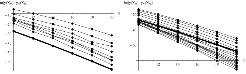
with M = 10 (i.e. h = 1), and N = 10,12, . . . ,20. To explain the dependence between the global error and N, we plot in Fig. 2 the pairs {(N,ln|er_N(x_m)|);N = 10,12, . . . ,20}, for each m= 1,2, . . . ,M, (M=10 and 20). It is observed that the error decays exponentially with respect to N, in accordance with an earlier result given in [1], i.e.

error of ELGT(M,N)∼ 1 N!cN

N

wherecN

N is the leading coefficient of LN(x) in [0,1].

7

Nonlinear Differential Equations

Consider nonlinear ODEs of the form

12 14 16 18 20 N

60

50

40

30

20

10 lnyXmyNXm

12 14 16 18 20 N

60

40

20 lnyXmyNXm

Figure 2: (Example 5.) The order of ELGT(M,N) vis-avis N: Variations with N of ln|y(xm)−yN(xm)|compared to

the (heavy) plot of ln|_N!1_cN

N|, N=10,12, . . . ,20 and m=1,2,...,8 and M=10 (left), M=20 (right).

xm er_N(x_m)

N=10 N=12 N=14 N=16 N=18 N=20

1 7.34E-9 -9.62E-13 -8.55E-16 -4.45E-20 1.03E-23 4.45E-28 2 -9.81E-8 -1.70E-11 1.43E-14 5.34E-18 3.83E-22 -4.76E-26 3 3.19E-7 2.01E-10 1.45E-14 -3.03E-17 -1.14E-20 -1.57E-24 4 -3.05E-7 -4.79E-10 -2.90E-13 -5.93E-17 -9.77E-22 8.48E-26 5 -8.71E-7 7.85E-10 3.56E-12 1.86E-15 -1.79E-18 -5.04E-22 6 2.54E-6 1.40E-8 -2.58E-11 -1.42E-13 1.18E-17 1.69E-19 7 -1.87E-4 4.89E-7 -3.51E-9 1.09E-11 8.77E-15 4.90E-18 8 2.34E-2 -2.70E-4 1.72E-6 -5.94E-9 1.33E-11 -1.95E-14 9 1.30E-1 1.03E-4 -2.30E-5 2.89E-7 -1.74E-9 6.02E-12 10 -4.98E1 -4.31E-1 9.78E-3 -1.26E-4 9.98E-7 -5.03E-9

Table 4: (Example 5.) Exact error er_N(x_m) at some pointsxmforh= 1 forN = 10,12, ...,20.

y(a) =α0, y(a) =α1.

To approximate the exact solutiony by means of ELGT we follow the following procedure:

Take a partition a =x0 < x1 < . . . < xM = b of [a,b]

and seth=xi−xi−1.

On each [x_i−1, xi], apply ELGT iteratively to linear IVPs,

y_k−f_yy_k−f_yy_k=f(x, y_k−1, y_k−1)−fyy

k−1−fyyk−1+O(e2), wheree(x) =y−y_k−1, and{f_y, f_y, f_yy, f_yy, f_yy}are

evaluated at (y_k−1, y_k−1).

For smallh, one can safely dropO(e2).

For each cycle, constructyk. Repeat the process until a

prescribed convergence toleranceis satisfied.

Example 6. _{Consider the nonlinear problem [5]}

y+y+y3= (cosx+ sin(10x))3−99sin(10x), x≥0, y(0) = 1, y(0) = 10,

whose the exact solution is y(x) = cosx+sin(10x). I solved this problem over [0,200] and measured the error atx= 100 andx= 200. The results are given in Table 3.

M h x_m ELGT[M,4,0] ELGT[M,4,6]

400 0.5 100.0 1.96E-5 1.60E-6 800 0.25 100.0 2.31E-8 6.20E-10 1600 0.125 100.0 6.90E-11 2.74E-13

400 0.5 200.0 9.04E-6 8.31E-7 800 0.25 200.0 1.16E-8 4.68E-10 1600 0125 200.0 3.36E-11 2.18E-13

Table 5: (Example 6.) The error at the mid-point and end-point of [0,200] obtained by ELGT[M,4,K] forM = 400,800,1600 and K= 0,6.

Example 7. _{The following nonlinear problem was} stud-ied in Papeorgiou et al [10]

y+ 100y= siny, x≥0, y(0) = 0, y(0) = 1.

Exact y(x) is not available, but exact y(20π) = 0.000392823991. We applied ELGT in [0,20π] and re-ported the errors atx= 20πin Table 6.

ELGT(M,4) Papageorgiou Tsitouras and

et al[10] Simos [13] M steps Error M steps Error F. Ev. Error

100 2.66E-4 2400 5.63E-4 200 9.13E-6 4800 9.29E-6

400 6.04E-8 7200 8.24E-7 12000 2.6E-11 800 2.69E-10 14000 3.6E-11 1600 1.50E-12 16000 5.8E-12

Table 6: (Example 7.) The error at x = 20π for the ELGT and [10].

Example 8. _{(Duffing problem). The exact solution of}

y+y+y3=Fcos(Ωx), x≥0, y(0) =yG(0), y

is given byyG(x) =

_∞

i=0α2i+1cos((2i+ 1)Ωx), where α1 = 0.200179477536, α3 = 0.246946143E−3, α5 = 0.304014E−6,α7= 0.374E−9,α9, α11, . . . <10−12.

I solved this problem in [0,20π] withF = 0.002 and Ω = 1.001 for M=50, 100 and 200. The maximum errors over [0,20π] were computed and listed in Table 7. My results are compared to those obtained by the five stage method introduced in [10]. I also solved the Duffing problem in

ELGT(M,4) Papageorgiou_{et al}[10] M steps Error M steps Error

50 5.41E-06 600 4.31E-07 100 2.25E-08 1200 6.56E-09 200 9.15E-11 2400 1.05E-10

Table 7: (Example 8.) Maximum errors over [0,20π] for ELGT compared to those given in [10].

interval [0,300] with several number of steps. The results are listed in Table 8.

Error at_x= 300

M steps ELGT Ixaru and Vanden Simos [13] Berghe [5]

300 6.25E-7 1.10E-3 1.70E-3 600 2.78E-9 5.42E-5 1.88E-4 1200 1.31E-11 1.86E-6 1.37E-5 2400 6.19E-8 8.70E-7 4800 2.40E-9 5.41E-8

Table 8: (Example 8.) The Euclidean norm of the global error at the end-pointx= 300 of [0,300] for ELGT and EFERKM of Ixaru and Vanden Berghe [5] and by Simos’s method given in Simos [13], [14].

8

Conclusions and Future Work

In this paper, an exponentially weighted Legendre-Gauss Tau Method for approximating ODEs with strongly oscil-latory solution is developed. ELGT involves some weights with frequencies {ω} being the roots of the quadratic equation associated with the constant reference equation. The new method is capable of detecting the sharp vari-ations of the function throughout a considerably large interval of integration. The accuracy of ELGT can be measured either in terms of the step sizeh or in terms ofN, the degree Legendre polynomialL_N. In the former we obtain an error of orderO(h2m_{) and the latter results}

in error of orderO(_N1_!).

ELGT needs to be tested on Sturm-Liouville problems, both regular and irregular. A comprehensive treatment for systems of nonlinear ODEs is not presented here, but it is possible using Alekseev-G´obner lemma.

References

[1] El-Daou, M.K. and Ortiz, E.L.,“Error analysis of the tau method: dependence of the error on the degree and on the length of the interval of approximation”,

Comput. Math. ApplsV25, pp.33-45, 1993.

[2] El-Daou, M.K., “Computable error bounds for coef-ficients perturbation methods”,ComputingV69, pp. 305-317, 2002.

[3] Gottlieb, D. and Orszag, S.A.,Numerical Analysis of Spectral Methods: Theory and Applications, Series in Appl. Math., SIAM, Philadelphia, Pa., 1977.

[4] Ixaru, L.Gr., Numerical Methods for Differential Equations and Applications, D.Reidel Publishing Co, Dordrecht, 1984.

[5] Ixaru, L.Gr., Vanden Berghe, G., Exponential Fit-ting, Kluwer Academic Publishers, Dordrecht, 2004

[6] Lambert, J.D.,Computational Methods in Ordinary Differential Equations, John Wiley and Sons, Lon-don, 1973.

[7] Lanczos, C.,Applied Analysis, Prentice-Hall, Engle-wood Cliffs, New Jersy, 1956.

[8] Ledoux, V., Rizea, M., Ixaru, L.Gr., Vanden Berghe, G., Van Daele, M., “Solution of the Schr¨odinger equation by a high order perturbation method based on linear reference potential”,Comput. Phys. Com-mun., N175, pp. 424-439, 2006.

[9] Ortiz, E.L., “The Tau Method”, SIAM J. Numer. Anal., V6, pp. 480-492, 1969.

[10] Papageorgiou, G., Famelis, I.Th., Tsitouras, Ch., “A P-stable diagonally implicit Runge-Kutta-Nystr¨om method” Numerical Algorithms, V17 pp. 345-353, 1998.

[11] Pruess S., “Estimating the eigenvalues of Sturm-Liouville problems by approximating the differential equations”,SIAM J. Numer. Anal.V10, pp. 55-68, 1973.

[12] Pryce, J.D.,Numerical Solution of Sturm-Liouville Problems, Clarendon Press, Oxford Science Publi-cations, 1993.

[13] Simos T.E., “An exponentially-fitted Runge-Kutta method for the numerical integration of initial-value problems with periodic or oscillating solutions”,

Comput. Phys. Comm.,V115, pp. 1-8, 1998.