Abstract—Conventional neural network training methods find a single set of values for network weights by minimizing an error function using some gradient descent-based technique. In contrast, the Bayesian approach infers the posterior distribution of weights, and makes predictions by averaging the predictions over a sample of networks, weighted by the posterior probability of the network given the data. The integrative nature of the Bayesian approach allows it to avoid many of the difficulties inherent in conventional approaches. This paper reports on the application of Bayesian MLP techniques to the problem of predicting the direction in the movement of the daily close value of the Australian All Ordinaries financial index. Predictions made over a 13 year out-of-sample period were tested against the null hypothesis that the mean accuracy of the model is no greater than the mean accuracy of a coin-flip procedure biased to take into account non-stationarity in the data. Results show that the null hypothesis can be rejected at the 0.005 level, and that the t-test p-values obtained using the Bayesian approach are smaller than those obtained using conventional MLPs methods.
Index Terms—Direction-of-change forecasting, Financial time series, Markov Chain Monte Carlo, Neural Networks.
I. INTRODUCTION
Predicting the future value of a time series based on historical values is usually approached as an auto-regression problem in which the parameters of the model are first optimized using in-sample data; the model is then used to make forecasts on a set of out-of-sample data; and the accuracy of the forecasts is finally measured by comparing the forecast values with the realized (i.e., actual) values. In many cases, however, correctly predicting the direction of the change (i.e., up or down) is a more important measure of success. For example, if a trader is to make buy/sell decisions on the basis of forecast values, it is more important to be able to correctly predict the direction of change than it is to achieve, say, a small mean squared error. We call this direction-of-change forecasting, and its importance has been acknowledged in several recent papers [1]-[4].
Clearly, if one has made a prediction for the future value of a time-series, then that prediction can trivially be converted into a direction-of-change prediction by simply predicting up/down if the forecast value is greater/smaller than the present value. There may, however, be advantages in predicting the direction-of-change directly (i.e., without explicitly predicting the future value of the series). For
Manuscript received March 13, 2008. A. Skabar is with the Department of Computer Science and Computer Engineering, La Trobe University, Bundoora, Australia. (phone: (+61) 3 9479 2598; fax: (+61) 3 9479 3060; e-mail: [email protected]).
example, traders base their decisions primarily on their opinion of whether the price of a commodity will rise or fall, and to a lesser extent on their opinion of the degree to which it will rise or fall. This may create in financial systems an underlying dynamic that allows the direction of change to be predicted more reliably than the value of the series. In this paper, we perform direction-of-change forecasting using Multilayer Perceptrons (MLPs) as binary classifiers.
Conventional MLP training methods attempt to find a single set of values for the network weights by minimizing an error function using some gradient descent based technique. The error function is usually chosen such that the resulting network represents the most probable network given the data, and following Bishop (1995), we refer to this as the maximum likelihood (ML) approach [5]. In order to prevent overfitting, and thus achieve good predictive performance on holdout data, the network should have an appropriate number of hidden layer units, and the error function should usually include a regularization term. Model parameters such the number of hidden units and the value of the regularization coefficients should be determined before the final network is trained, and a validation procedure is usually used to determine these values.
In contrast to the ML approach, Bayesian MLP methods [6-8] do not attempt to find a single ‘best’ weight vector;but rather, they attempt to infer the posterior distribution of the weights, given the data. Samples can then be taken from this distribution, each sample representing a distinct MLP. Given some novel example, each of the sampled networks can be applied to the example, with the resulting prediction being the average prediction over the sample of networks weighted by the posterior probability of the network given the training data. Thus, whereas the conventional approach optimizes over parameters, the Bayesian approach integrates over parameters, and this allows it to avoid many of the difficulties that conventional approaches have in avoiding overfitting.
This paper reports on the application of Bayesian MLP methods to the financial prediction problem, and expands on preliminary results that have been presented in [9]. Section 2 describes the neural network approach to the problem of financial prediction, and highlights some of the problems that conventional MLP approaches have in this domain. Section 3 describes the Bayesian MLP approach, and Section 4 presents empirical results of applying Bayesian MLP techniques to predicting the direction of change in daily close value of the Australian All Ordinaries index. The results are discussed in Section 5, and Section 6 concludes the paper.
Direction-of-Change Financial Time Series
Forecasting using Bayesian Learning for MLPs
II. MLPS FOR FINANCIAL PREDICTION
A multilayer perceptron (MLP) is a function of the following form:
0 1
0 0
( ) ( ) where
N N
n n
kj ji i
j i
f h u u w g w x
= =
= =
∑
∑
x (1)
where N0 is the number of inputs (i.e., the dimensionality of the input feature vector), N1is the number of units in a hidden layer, wji is a numerical weight connecting input unit i with hidden unit j, wkj is the weight connecting hidden unit j with output unit k, h(u) = σ(u) ≡ (1 + exp(−u))−1 (i.e., a sigmoid function), and g(u) is either a sigmoid, or some other continuous, differentiable, nonlinear function. Thus, an MLP with some given architecture, and weight vector w, provides a mapping from an input vector x to a predicted output y given by y = f (x, w). Given some data, D, consisting of n independent items (x1, y1), …, (xN, yN), the objective is to find asuitable w.
In the case of financial prediction, the raw data usually consists of a series of values measured at regular time intervals; e.g. the daily close value of a financial index such as the Australian All Ordinaries. The input vector, xN, corresponds to the Nth value of the series, and usually consists of the current value, in addition to time lagged values, or quantities which can be derived from the series, such as moving averages.
One approach is to use the MLP to predict the next value of the series. This is a regression problem, as the objective is to predict a continuous-valued quantity; i.e., the price of a stock, or the close value of an index. In this case, the appropriate error function to be minimized is the quadratic error between target and predicted outputs. This is justified under the assumption that the training examples are normally distributed around the target function with zero mean and constant variance.
The other approach, and the approach taken in this paper, is to predict only the direction of the change. In order to do this, one could simply take the regression approach described above, and compare the predicted (continuous) value against the current value to determine the direction of change. However, an alternative approach is to treat the problem as a binary classification problem. In this case, the training examples are labelled with binary target values representing the direction of change from the previous day’s value. In order for the MLP to represent the probability of an upwards change (target value of 1), the MLP should be trained so as to minimize the cross-entropy error, and is described in greater detail in the next section.
The conventional approach to finding the weight vector w
is to use a gradient-descent method to find a weight vector that minimizes the error between the network output value, f (x,
w), and the target value, y. This approach is generally referred to as the maximum likelihood (ML) approach because it attempts to find the most probable weight vector, given the training data. This weight vector, wML, is then used to predict the output value corresponding to some new input vector xn+1.
One of the main difficulties in applying MLPs to the
financial prediction domain concerns the very high level of noise in the data, and thus the danger of overfitting the network. The main issue is how to optimize model parameters, such as the number of hidden units and regularization coefficient, so as to minimize the degree of overfitting on the training data. One approach is to use an independent validation set to optimize these parameters. The main difficulty here is how to select examples for the validation set. For example, if these are chosen to be adjacent to, but between, the training and test sets, then any patterns found in the training data may have dissipated before the model is applied to the test data. Moreover, because the validation set is itself noisy, there will be considerable uncertainty in whether the parameters values chosen are indeed optimal. An alternative approach is to omit the validation set, and select parameters that provide the best results on the test data, but in this case we can never be sure that we have not simply optimized these parameters to the test set.
III. BAYESIAN METHODS FOR MLPS
In contrast to the ML approach, Bayesian methods for MLPs do not attempt to find a single ‘best’ weight vector w; rather, they infer p(w|D), the posterior distribution of the weights given the data. The predicted output corresponding to some input vector xn is then obtained by performing a weighted sum of the predictions over all possible weight vectors, where the weighting coefficient for a particular weight vector depends on p(w|D). Thus,
ˆn ( n ( | )
y =
∫
f x w), p w D dw (2)where f(xn, w) is the MLP output. The fact that p(w|D) is a probability density function allows us to express the integral in Equation 2 as the expected value of f(xn, w) over this density:
( | )
1
( , ) ( | ) ( , )
1
( , ) w
x w w w x w
x w
n n
p D N
n i
f p D d E f
f N =
=
∫
∑
≃
(3)
Thus, the integral can be estimated by drawing N samples from the density p(w|D), and averaging the predictions due to these samples. This process is known as Monte Carlo integration.
The density p(w|D) can be estimated using the fact that
( ) ( | ) ( )
pw |D ∝p D w pw , where p(w| D) is the likelihood, and p(w) is the prior weight distribution. If the target values are binary, then the likelihood can be expressed as
{
}
( |w) exp nln (xn,w) (1 ) ln(1n (xn,w))
n
p D =
∑
t f + −t −f (4)The prior weight distribution, p(w), should reflect any prior knowledge that we have about the complexity of the MLP. To reflect the fact that we want it to be a smooth function, p(w) is commonly assumed to be Gaussian with zero mean and inverse variance α, giving preference to weights with smaller magnitudes; i.e.,
/ 2
2
( ) exp
2 2
m m
i i=1
p α α w
π
= −
∑
w (5)
where m is the number of weights in the network [12]. However, we usually do not know what variance to assume for the prior distribution, and for this reason it is common to set a distribution of values. As α must be positive, a suitable form for its distribution is the gamma distribution [12]. Thus,
/ 2 / 2 1
( / 2 )
( ) exp( / 2 )
( / 2) a
a a
p a
a
µ
α = α − −α µ
Γ (6)
where the a and µ are respectively the shape and mean of the gamma distribution, and are set manually. Note that a single α need not be used for all weights and biases. For example, it is common to use separate values of α for input-hidden-layer weights, input-to-hidden-layer biases, hidden-to-output layer weights, and hidden-to-output layer biases, which is the approach taken in this paper, and in which we denote the respective weight groupings as α1, α2, α3, and α4 respectively. Note that each weight grouping will have its own distribution parameterised by ai and µi, where ai and µi represent the shape and mean for the respective group. We discuss methods for selecting appropriate values for a and µ in the next section.
Because the prior depends on α, Equation 2 should be modified such that it includes the posterior distribution over the α parameters:
ˆn ( n ( , | )
y =
∫
f x w), p wα D d dw α (7)where
( , ) ( | ) ( , )
p wα|D ∝p D w p wα (8)
Monte Carlo integration depends on the ability to obtain samples from the posterior distribution. The objective is to sample preferentially from the region where p(w,α| D) is large. The Metropolis algorithm [10] achieves this by generating a sequence of vectors in such a way that each successive vector depends on the previous vector as well as having a random component; i.e., wnew = wold + ε, where ε is a small random
vector. Preferential sampling is then achieved using the criterion:
new old
new
new old
old
if ( | ) ( | ) accept
( | )
if ( | ) ( | ) accept with probability
( | )
p D p D
p D
p D p D
p D
> <
w w
w
w w
w
The difficulty in using the Metropolis algorithm to estimate the integrals for neural networks stems from the strong
correlations in the posterior weight distribution; i.e., the great majority of the candidate steps generated in the random walk will be rejected as they lead to a decrease in p(w|D) [5]. The Hybrid Monte Carloalgorithm [11] reduces the random walk behaviour by using gradient information, which, in the case of MLPs, can be readily calculated. While the Hybrid Monte Carlo algorithm allows for the efficient sampling of parameters (i.e., weights and biases), the posterior distribution for αshould also be determined. In this paper we use Neal’s (1996) approach, and use Gibbs sampling [12] for the αs.
IV. EMPIRICAL RESULTS
The experimental results reported in this section were obtained by applying the techniques described previously to the daily close values of the Australian All Ordinaries Index (AORD) for the period from November 1990 to December 2004. The task is to predict the direction of movement (up or down) of the close value on day t+1 from historical close values. Specifically, we are interested in the proportion of test examples for which the direction in movement is predicted correctly, and we refer to this as the sign correctness proportion (SCP). The SCP is defined as follows:
1
1
k k
N t o k SCP
N =δ
=
∑
(9)where N is the number of test examples in the prediction period, tk and ok are the binary target and network outputs respectively, and δij = 1 if i = j, and 0 otherwise. Note that because the network output represents the probability of an upward movement, the binary output, ok, is obtained by thresholding the output at 0.5.
The time series is shown in Figure 1, in which days 0 and above are those for which prediction were made, and days prior to day 0 were used for preprocessing. In total, 3600 predictions were made. Note that the series is clearly non-stationary.
A. Feature Selection and Preprocessing
Almost invariably, successful financial forecasting requires that some preprocessing be performed on the raw data. This usually involves some type of transformation of the data into
-500 0 500 1000 1500 2000 2500 3000 3500 1000
1500 2000 2500 3000 3500 4000 4500
day
v
a
lu
[image:3.595.316.539.620.758.2]e
new variables more amenable to learning from. Thus, rather than using, for example, the past prices of a stock, transformed variables might include the absolute change in the price, (pt – pt –1), the rate of change of price, (pt – pt –1) / pt
–1, or the price or change in price relative to some index or
other baseline such as a moving average [3]. The advantage of using variables based on changes in price (either relative or absolute) is that they help to remove non-stationarity from the time series.
In this study, the input variables used are the relative change in close value from the previous day to the current day (r1), and the 5, 10, 30 and 60 day moving averages (ma5, ma10, ma30, ma60). The moving averages are calculated by simply averaging the x previous closing values, where x is the period of the moving average. Thus, the input to the network is the vector ( r1(t), ma5(t), ma10(t), ma30(t), ma60(t) ) where
(
)
( ) /
n t t n t
r t = p −p− p (10)
and
1 ( )
t
n t
t n
ma t p
n −
=
∑
(11)Note that there would almost certainly exist some other combination of inputs and preprocessing steps that might lead to better performance than that which can be achieved using this particular combination. However, in this paper we are not concerned with optimizing this choice of inputs; rather, we are concerned with comparing the performance of the Bayesian approach with that of the ML approach. If the Bayesian approach is found to give superior performance, this is very unlikely to be due to this particular choice of inputs.
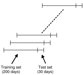
B. Training and Prediction Windows
A prediction window period of 30 days was used in this study, with the training set for each 30-day prediction period consisting of data for the 200 trading days immediately preceding the test period. A total of 120 30-day predictions were made (i.e., 3600 days), with the training and test windows advanced by 30 days after each 30-day prediction period. This is depicted in Figure 2.
The choice of 200 days for training was based on the assumption that patterns that exist in the training may dissipate after some time, and hence that data temporally far removed from the prediction period may not be useful. In principle, the test window could consist of a single prediction, but this would increase the computational cost 30-fold. Also, the particular hypothesis testing scheme that we use requires that the test window consists of multiple predictions (see below).
C. Hypothesis Testing
Assuming that a return series is stationary, then a coin-flip decision procedure for predicting the direction of change would be expected to result in 50% of the predictions being correct. We would like to know whether our model can produce predictions which are statistically better than 50%.
Training set (200 days)
[image:4.595.356.491.49.171.2]Test set (30 days)
Fig. 2. Training and test windows. Windows are advanced by 30 days after each 30-day prediction is made
However, a problem is that many financial return series are not stationary, as evidenced by the tendency for commodity prices to rise over the long term. This is clearly visible in Fig 1, where there is a clear upward trend over the period shown, suggesting that the total number of upwards movements is greater than the number of downward movements.Thus it may be possible to achieve an accuracy significantly better than 50% by simply biasing the model to always predict up.
A better approach is to compensate for this non-stationarity, and this can be done as follows. Let xa represent the fraction of days in an out-of-sample test period for which the actual movement is up, and let xp represent the fraction of days in the test period for which the predicted movement is up. Therefore under a coin-flip model the expected fraction of days corresponding to a correct upward prediction is (xa × xp), and the expected fraction of days corresponding to a correct downward prediction is (1−xa) × (1−xp). Thus the expected fraction of correct predictions is
aexp = (xa×xp) + ((1−xa) × (1−xp)) (12)
We wish to test whether amod (the accuracy of the predictions of our model) is significantly greater than aexp (the compensated coin-flip accuracy). Thus, our null hypothesis may be expressed as follows:
Null Hypothesis: H0 : amod≤aexp H1 : amod > aexp
The null hypothesis can be tested by performing a paired t-test of the samples obtained from each of the 120 30-day prediction periods, comparing the means of amod and aexp.
D. Setting the Prior Distribution
The Bayesian approach requires that we specify the prior weight distribution, p(w). Recall that p(w) is assumed to be Gaussian, with inverse variance α, and that α is assumed to be distributed according to a Gamma distribution with shape a and mean µ., which remain to be specified. In order to gain some insight into the range of values may be suitable for these parameters, we conducted a number of trials using the ML approach, with weight optimization performed using the scaled conjugate gradients algorithm.
obtained through performing the t-test. Italics show best performance.
Figure 3 plots training and test set accuracies against the α value. Low values for α, such as 0.01, impose a small penalty for large weights, and result in overfitting; i.e., high accuracy on training data, but low accuracy on test data. In this case, the null hypothesis cannot be rejected at the 0.05 level. In contrast, when αis very high (e.g., 10.0), large weights will penalised more heavily, leading to weights with small magnitudes. In this case the MLP will be operating in its linear region and the MLP will display a strong bias towards predictions that are in the same direction as the direction of the majority of changes on the training data. Thus, if the number of upward movements on the training data is greater than the number of negative movements, the MLP will be biased towards making upwards predictions on the test data; however, this is not likely to lead to a rejection of the null hypothesis because the null hypothesis takes the non-stationarity of the data into account. It can be seen from Figure 3 that a local maximum for the test set accuracy occurs
TABLE I.
TRAIN ACCURACY,TEST ACCURACY AND P-VALUE FOR VARIOUS α VALUES
α value Train. Acc. Test. Acc. p-value (Ho)
0.010 0.725 0.490 0.402
0.100 0.701 0.501 0.459
0.500 0.608 0.516 0.169
0.750 0.593 0.520 0.070
1.000 0.585 0.524 0.007
1.500 0.570 0.521 0.038
2.000 0.562 0.518 0.587
5.000 0.549 0.526 0.528
10.00 0.542 0.525 0.479
0.45 0.50 0.55 0.60 0.65 0.70 0.75
0.0 1.0 2.0 3.0 4.0 5.0 6.0 7.0 8.0 9.0 10.0
alpha (inverse variance of w eights)
A
c
c
u
ra
c
y
Average Training Accuracy Average Testing Accuracy
Fig. 3. Training and test set accuracy averaged over 120 training/test set pairs. A local maximum test accuracy corresponds to an α value of approximately 1.0
0 0.5 1 1.5 2 2.5 3
0 0.5 1 1.5
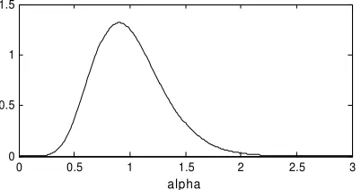
[image:5.595.70.271.671.777.2]alpha
Fig. 4. Gamma distribution with mean 1.0 and shape parameter value 10
for an α value of 1.0, and in this case the null hypothesis can clearly be rejected at the 0.01 level.
The range of α values for which the null hypothesis can be rejected is very narrow, and ranges from a lower α value in the vicinity of 0.5 to 0.75, to a an upper α value in the vicinity of 1.5 to 2.0. After visualizing the pdf for Gamma distributions with mean 1.0 and various values for the shape parameter, a shape parameter of 10 was chosen. The pdf is shown in Figure 4. Note that the pdf conforms roughly to the α value identified in the Table I as leading to a rejection of the null hypothesis.
E. MCMC sampling
We now describe the application of the Bayesian approach, which relies on MCMC sampling to draw weight vectors from the posterior weight distribution.
Monte Carlo sampling must be allowed to proceed for some time before the sampling converges to the posterior distribution. This is called the burn-in period. In the results presented below, we allowed a burn-in period of 1000 samples, following which we then saved every tenth sample until a set of 100 samples was obtained. Each of the 100 samples was then applied to predicting the probability of an upwards change in the value of the index on the test examples, and the probabilities were then averaged over the 100 samples. The resulting p-values are shown in Table II, together with the results from Table I corresponding to an α value of 1.0; i.e., the performance of the best network trained using the conventional approach. Note that the p-values are now much smaller, indicating increased confidence in the rejection of the null hypotheses, and that the average test accuracy has increased from 52.4% to 52.8%. Also note that the average training accuracy for the Bayesian approach is less than that for the ML approach, thereby supporting the claim that the Bayesian approach is better at avoiding overfitting.
V. DISCUSSION
The superior performance of the Bayesian approach can be attributed to its integrative nature: each individual weight vector has its own bias, and by integrating over many weight vectors, this bias is decreased, thus reducing the likelihood of inferior generalization performance resulting from overfitting on the training data.
The Bayesian technique assumes that the MCMC sampling has proceeded for a sufficient time such that the convergence to the true posterior distribution has been achieved; however, there are currently no adequate techniques available for testing convergence. We experimented with starting the MCMC sampling from various starting weight vectors. Specifically, we compared the results of starting the sampling
TABLE II
TRAIN ACCURACY,TEST ACCURACY AND P-VALUE FOR CONVENTIONALLY TRAINED (SCG) AND BAYESIAN-TRAINED (MCMC)MLPS Method Train. Acc. Test. Acc. p-value (Ho)
SCG 0.585 0.524 0.0068
[image:5.595.311.541.747.778.2]from a random point, with results of sampling from a minima found by applying the ML approach, and found that after the 1000 sample burn-in period there was no significant difference in results. While this is not conclusive evidence that the sampling has converged, it does indicate that the 1000 sample burn-in period is sufficient to bring the sampling into the region of weight space corresponding to a local minimum, and probably close to the global minimum.
The most important decision to be made in using the Bayesian approach is the choice of prior. In this study, we used a relatively narrow distribution for α, the parameter controlling the degree of regularization present in the error function. This choice was made based on experimenting with different α values within the ML approach. The criticism could be made that this prior distribution was selected based on the same data that we had used for testing, and hence that the significance of our results may be overstated; however, this is unlikely to be the case, as the prior depends on factors such as the degree of noise in the data, and this is relatively constant over different periods of the same index. Consequently, it is very unlikely that using a different set of data would have resulted in a significantly prior. Moreover, the fact that we need only select parameters describing the distribution of α, rather than specific value for α, further diminishes the possibility that our prior is biased towards the particular dataset that we have used.
One of the advantages of the Bayesian approach is its inherent ability to avoid overfitting, even when using very complex models. Thus, although the results presented in this paper were based on MLPs with six hidden units, the same performance could, in principle, have been achieved using a more complex network. It is not clear, however, whether we should expect any coupling between the number of hidden layer units and the prior distribution. For this reason, we would recommend preliminary analysis using the ML approach to ascertain the appropriate range for α and selection of priors based on values which lead to significant predictive ability.
VI. CONCLUSION
Bayesian Learning for MLPs has been applied to predicting the next day’s close value of the Australian All Ordinaries index over a period of approximately 13 years. Predictions were tested against the null hypothesis that the mean accuracy of the model is no greater than the mean accuracy of a coin-flip procedure biased to take into account non-stationarity in the data. Results show that the null hypothesis can be rejected at the 0.005 level, and that the t-test p-values obtained using the Bayesian approach are approximately one fifth the value of those obtained using MLPs trained using the conventional ML approach. The superior performance of the Bayesian approach is due to its integrative nature, and its inherent ability to avoid overfitting.
REFERENCES
[1] Y. Kajitani, A.I. Mcleod, K.W. Hipel, "Forecasting nonlinear time series with feed-forward neural networks: a case study of Canadian lynx data," Journal of Forecasting 24, 2005, pp. 105–117, [2] J. Chung, Y. Hong, "Model-free evaluation of directional
predictability in foreign exchange markets,".Journal of Applied Econometrics 22, 2007, pp. 855–889.
[3] P.F. Christoffersen, F.X. Diebold, "Financial asset returns, direction-of-change forecasting, and volatility dynamics," PIER Working Paper Archive 04-009, Penn Institute for Economic Research, Department of Economics, University of Pennsylvania, 2003.
[4] S. Walczak, "An empirical analysis of data requirements for financial forecasting with neural networks," Journal of Management Information Systems, 17 (4), 2001, pp. 203-222.
[5] C. Bishop, Neural networks for pattern recognition, Oxford University Press, Oxford, 1995.
[6] D.J.C. MacKay, "A practical Bayesian framework for back propagation networks," Neural Computation, 4(3), 1992, pp. 448-472.
[7] R.M. Neal, "Bayesian Training of Backpropagation Networks by the Hybrid Monte Carlo Method," Technical Report CRG-TR-92-1, Department of Computer Science, University of Toronto, 1992. [8] R.M. Neal, Bayesian Learning for Neural Networks, New York:
Springer-Verlag, 1996.
[9] A. Skabar, "Application of Bayesian Techniques for MLPs to Financial Time Series Forecasting," Proceedings of 16th Australian Conference on Artificial Intelligence (AI 2005), 2005, pp. 888-891. [10] N.A. Metropolis, A.W. Rosenbluth, M.N. Rosenbluth, A. Teller and
E. Teller, "Equation of State Calculations by Fast Computing Machines," Journal of Chemical Physics 21(6), 1953, pp. 1087-1092. [11] S. Duane, A.D. Kennedy, B.J. Pendleton and D. Roweth, "Hybrid
Monte Carlo". Physics Letters B. 195(2), 1987, pp. 216-222. [12] S. Geman and G. Geman, G, "Stochastic Relaxation, Gibbs