Muli label Text Categorization with Hidden Components

Muli-label Text Categorization with Hidden Components

Li Li Longkai Zhang Houfeng Wang

Key Laboratory of Computational Linguistics (Peking University) Ministry of Education, China [email protected], [email protected], [email protected]

Abstract

Multi-label text categorization (MTC) is supervised learning, where a documen-t may be assigned widocumen-th muldocumen-tiple cadocumen-tegories (labels) simultaneously. The labels in the MTC are correlated and the correlation re-sults in some hidden components, which represent the ”share” variance of correlat-ed labels. In this paper, we propose a method with hidden components for MTC. The proposed method employs PCA to capture the hidden components, and incor-porates them into a joint learning frame-work to improve the performance. Experi-ments with real-world data sets and evalu-ation metrics validate the effectiveness of the proposed method.

1 Introduction

Many real-world text categorization applications are multi-label text categorization (Srivastava and Zane-Ulman, 2005; Katakis et al., 2008; Rubin et al., 2012; Nam et al., 2013), where a docu-ments is usually assigned withmultiplelabels si-multaneously. For example, as figure 1 shows, a newspaper article concerning global warming can be classified into two categories, Environmen-t, and Science simultaneously. Let X = Rd

be the documents corpus, and Y = {0,1}m _be

the label space with m labels. We denote by {(xxx111,yyy111),(xxx222,yyy222), ...,(xxxnnn,yyynnn)}the training set of ndocuments. Each document is denoted by a vec-torxxxi = [xi,1, xi,2, ..., xi,d]ofddimensions. The

labeling of thei-th document is denoted by vector

yyyi = [yi,1, yi,2, ..., yi,m], whereyil is 1 when the i-th document has thel-th label and 0 otherwise. The goal is to learn a functionfff :X → Y. Gener-ally, we can assume fff consists ofmfunctions, one for a label.

fff = [f1, f2, ..., fm]

Figure 1: A newspaper article concerning global warming can be classified into two categories, En-vironment, andScience.

The labels in the MLC are correlated. For ex-ample, a ”politics” document is likely to be an ”e-conomic” document simultaneously, but likely not to be a ”literature” document. According to the latent variable model (Tabachnick et al., 2001), the labels with correlation result in some hidden components, which represent the ”share” variance of correlated labels. Intuitively, if we can capture and utilize these hidden components in MTC, the performance will be improved. To implement this idea, we propose a multi- label text categorization method with hidden components, which employ PCA to capture the hidden components, and then incorporates these hidden components into a joint learning framework. Experiments with various da-ta sets and evaluation metrics validate the values of our method. The research close to our work is ML-LOC (Multi-Label learning using LOcal Cor-relation) in (Huang and Zhou, 2012). The

ences between ours and ML-LOC is that ML-LOC employs the cluster method to gain the local cor-relation, but we employ the PCA to obtain the hid-den code. Meanwhile, ML-LOC uses the linear programming in learning the local code, but we employ the gradient descent method since we add non-linear function to the hidden code.

The rest of this paper is organized as follows. Section 2 presents the proposed method. We con-duct experiments to demonstrate the effectiveness of the proposed method in section 3. Section 4 concludes this paper.

2 Methodology

2.1 Capturing Hidden Component via Principle Component Analysis

The first step of the proposed method is to capture hidden components of training instances. Here we employ Principal component analysis (PCA). This is because PCA is a well-known statistical tool that converts a set of observations of possibly correlat-ed variables into a set of values of linearly uncorre-lated variables called principle components. These principle components represent the inner structure of the correlated variables.

In this paper, we directly employ PCA to con-vert labels of training instances into their principle components, and take these principle components as hidden components of training instances. We denote byhhhithe hidden components of thei-th

in-stance captured by PCA.

2.2 Joint Learning Framework

We expand the original feature representation of the instancexxxiby its hidden component code

vec-torccci. For simplicity, we use logistic regression as

the motivating example. Letwwwldenote weights in

thel-th functionfl, consisting of two parts: 1)wwwxl

is the part involving the instance features. 2)wwwc l

is the part involving the hidden component codes. Henceflis:

fl(xxx,ccc) = _{1 + exp(−xxxT}1_wwwx

l −cccTwwwcl) (1)

whereCCC is the code vectors set of all training in-stances.

The natural choice of the code vector ccc is hhh. However, when testing an instance, the labeling is unknown (exactly what we try to predict), conse-quently we can not capturehhhwith PCA to replace the code vectorcccin the prediction function Eq.(1).

Therefore, we assume a linear transformationMMM

from the training instances to their independent components, and useMMMxxxas the approximate in-dependent component. For numerical stability, we add a non-linear function (e.g., the tanh function) toMMMxxx. This is formulated as follows.

ccc=tanh(MMMxxx) (2)

Aiming to the discrimination fitting and the in-dependent components encoding, we optimize the following optimization problem.

min

WWW ,C n X

i=1

m X

l=1

`(xxxi,ccci, yil, fl) +λ1Ω(fff)

+λ2Z(CCC) (3)

The first term of Eq.(3) is the loss function. `

is the loss function defined on the training data, andWWW denotes all weights in the our model, i.e.,

www1, ...,wwwl, ...,wwwm. Since we utilize the logistic

re-gression in our model, the loss function is defined as follows.

`(xxx,ccc, y, f)

= −ylnf(xxx,ccc)−(1−y)ln(1−f(xxx,ccc)) (4)

The second term of Eq.(3) Ω is to punish the model complexity, which we use the `2 regular-ization term.

Ω(fff) =

m X

l=1

||wwwl||2. (5)

The third term of Eq.(3)Zis to enforce the code vector close to the independent component vector. To obtain the goal, we use the least square error between the code vector and the independent com-ponent vector as the third regularized term.

Z(C) =Xn

i=1

||ccci−hhhi||2. (6)

By substituting the Eq.(5) and Eq.(6) into Eq.(3) and changingccctotanh(MMMxxx)(Eq.(2)), we obtain the following optimization problem.

min

W WW ,MMM

n X

i=1

m X

l=1

`(xxxi, tanh(MMMxxxi), yil,fff)

+λ1

m X

l=1

||wwwl||2+λ2

n X

i=1

||MMMxxxi−hhhiii||2

2.3 Alternative Optimization method

We solve the optimization problem in Eq.(7) by the alternative optimization method, which opti-mize one group of the two parameters with the other fixed. When theMMM fixed, the third term of Eq.(7) is a constant and thus can be ignored, then Eq.(7) can be rewritten as follows.

min

W W W

n X

i=1

m X

l=1

`(xxxi, tanh(MMMxxxi), yil, fl)

+λ1

m X

l=1

||wwwl||2 (8)

By decomposing Eq.(8) based on the label, the e-quation Eq.(8) can be simplified to:

min

w wwl

n X

i=1

`(xxxi, tanh(MMMxxxi), yil, fl) +λ1||wwwl||2 (9)

Eq.(9) is the standard logistic regression, which has many efficient optimization algorithms.

When WWW fixed, the second term is constan-t and can be omiconstan-tconstan-ted, constan-then Ep.(7) can rewriconstan-tconstan-ten to Eq.(10). We can apply the gradient descen-t medescen-thod descen-to opdescen-timize descen-this problem.

min

M M M

n X

i=1

m X

l=1

`(xxxi, tanh(MMMxxxi), yil, fl)

+λ2

n X

i=1

||MMMxxxi−hhhiii||2

(10)

3 Experiments

3.1 Evaluation Metrics

Compared with the single-label classification, the multi-label setting introduces the additional de-grees of freedom, so that various multi-label eval-uation metrics are requisite. We use three differen-t muldifferen-ti-label evaluadifferen-tion medifferen-trics, include differen-the ham-ming loss evaluation metric.

The hamming loss is defined as the percentage of the wrong labels to the total number of labels.

Hammingloss= _m1|h(xxx)∆yyy| (11)

where∆denotes the symmetric difference of two sets, equivalent to XOR operator in Boolean logic.

mdenotes the label number.

The multi-label 0/1 loss, also known as subset accuracy, is the exact match measure as it requires any predicted set of labelsh(xxx)to match the true set of labels Sexactly. The 0/1 loss is defined as follows:

0/1loss=I(h(xxx)6=yyy) (12)

Letaj andrjdenote the precision and recall for

thej-th label. The macro-averaged F is a harmon-ic mean between precision and recall, defined as follows:

F = _m1

m X

i=j

2∗aj∗rj

aj+rj (13)

3.2 Datasets

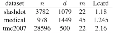
We perform experiments on three MTC data sets: 1) the first data set is slashdot (Read et al., 2011). The slashdot data set is concerned about science and technology news categorization, which pre-dicts multiply labels given article titles and partial blurbs mined from Slashdot.org. 2) the second da-ta set is medical (Pestian et al., 2007). This dada-ta set involves the assignment of ICD-9-CM codes to ra-diology reports. 3) the third data set is tmc2007 (S-rivastava and Zane-Ulman, 2005). It is concerned about safety report categorization, which is to la-bel aviation safety reports with respect to what types of problems they describe. The characteris-tics of them are shown in Table 1, wherendenotes the size of the data set,ddenotes the dimension of the document instance, andmdenotes the number of labels.

dataset n d m Lcard

slashdot 3782 1079 22 1.18

medical 978 1449 45 1.245

tmc2007 28596 500 22 2.16

Table 1: Multi-label data sets and associated statis-tics

The measure label cardinality Lcard, which is one of the standard measures of ”multi-label-ness”, defined as follows, introduced in (T-soumakas and Katakis, 2007).

Lcard(D) =

P_n

i=1Pmj=1yji n

whereDdenotes the data set, li

j denotes thej-th

3.3 Compared to Baselines

To examine the values of the joint learning frame-work, we compare our method to two baselines. The baseline 1 eliminates the PCA, which just adds an extra set of non-linear features. To im-plement this baseline, we only need to setλ2 = 0. The baseline 2 eliminates the joint learning frame-work. This baseline captures the hidden compo-nent codes with PCA, trains a linear regression model to fit the hidden component codes, and u-tilizes the outputs of the linear regression model as features.

For the proposed method, we set λ1 = 0.001 andλ2 = 0.1. For the baseline 2, we employ l-ogistic regression with 0.001 `2 regularization as the base classifier. Evaluations are done in ten-fold cross validation. Note that all of them pro-duce real-valued predictions. A thresholdtneeds to be used to determine the final multi-label setyyy

such thatlj ∈yyywherepj ≥t. We select threshold t, which makes theLcardmeasure of predictions for the training set is closest to the Lcard mea-sure of the training set (Read et al., 2011). The thresholdtis determined as follows, whereDtis

the training set and a multi-label model Ht

pre-dicts for the training set under thresholdt.

t= argmin

t∈[0,1] |Lcard(Dt)−Lcard(Ht(Dt))| (14)

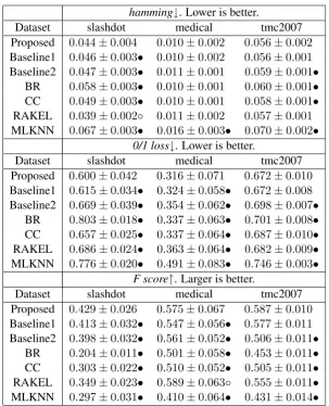
Table 2 reports our method wins over the base-lines in terms of different evaluation metrics, which shows the values of PCA and our join-t learning framework. The hidden componenjoin-t code only fits the hidden component in the baseline method. The hidden component code obtains bal-ance of fitting hidden component and fitting the training data in the joint learning framework.

3.4 Compared to Other Methods

We compare the proposed method to BR, C-C (Read et al., 2011), RAKEL (Tsoumakas and Vlahavas, 2007) and ML-KNN (Zhang and Zhou, 2007). entropy. ML-kNN is an adaption of kNN algorithm for multilabel classification. methods. Binary Revelance (BR) is a simple but effective method that trains binary classifiers for each label independently. BR has a low time complexity but makes an arbitrary assumption that the labels are independent from each other. CC organizes the classifiers along a chain and take predictions pro-duced by the former classifiers as features of the

latter classifiers. ML-kNN uses kNN algorithms independently for each label with considering pri-or probabilities. The Label Powerset (LP) method models independencies among labels by treating each label combination as a new class. LP con-sumes too much time, since there are 2m _label

combinations with m labels. RAndom K labEL (RAKEL) is an ensemble method of LP. RAKEL learns several LP models with random subsets of sizekfrom all labels, and then uses a vote process to determine the final predictions.

For our proposed method, we employ the set-up in subsection 3.3. We utilize logistic regression with 0.001`2 regularization as the base classifier for BR, CC and RAKEL. For RAKEL, the num-ber of ensemble is set to the numnum-ber of label and the size of the label subset is set to 3. For MLKN-N, the number of neighbors used in the k-nearest neighbor algorithm is set to 10 and the smooth pa-rameter is set to 1. Evaluations are done in ten-fold cross validation. We employ the threshold-selection strategy introduced in subsection 3.3

Table 2 also reports the detailed results in terms of different evaluation metrics. The mean metric value and the standard deviation of each method are listed for each data set. We see our proposed method shows majorities of wining over the other state-of-the-art methods nearly at all data sets un-der hamming loss, 0/1 loss and macro f score. E-specially, under the macro f score, the advantages of our proposed method over the other methods are very clear.

4 CONCLUSION

Many real-world text categorization applications are multi-label text categorization (MTC), where a documents is usually assigned withmultiplelabels simultaneously. The key challenge of MTC is the label correlations among labels. In this paper, we propose a MTC method via hidden components to capture the label correlations. The proposed method obtains hidden components via PCA and incorporates them into a joint learning framework. Experiments with various data sets and evaluation metrics validate the effectiveness of the proposed method.

Acknowledge

Tech-hamming↓. Lower is better.

Dataset slashdot medical tmc2007

Proposed 0.044±0.004 0.010±0.002 0.056±0.002 Baseline1 0.046±0.003• 0.010±0.002 0.056±0.001 Baseline2 0.047±0.003• 0.011±0.001 0.059±0.001•

BR 0.058±0.003• 0.010±0.001 0.060±0.001• CC 0.049±0.003• 0.010±0.001 0.058±0.001• RAKEL 0.039±0.002◦ 0.011±0.002 0.057±0.001 MLKNN 0.067±0.003• 0.016±0.003• 0.070±0.002•

0/1 loss↓. Lower is better.

Dataset slashdot medical tmc2007

Proposed 0.600±0.042 0.316±0.071 0.672±0.010 Baseline1 0.615±0.034• 0.324±0.058• 0.672±0.008 Baseline2 0.669±0.039• 0.354±0.062• 0.698±0.007•

BR 0.803±0.018• 0.337±0.063• 0.701±0.008• CC 0.657±0.025• 0.337±0.064• 0.687±0.010• RAKEL 0.686±0.024• 0.363±0.064• 0.682±0.009• MLKNN 0.776±0.020• 0.491±0.083• 0.746±0.003•

F score↑. Larger is better.

Dataset slashdot medical tmc2007

Proposed 0.429±0.026 0.575±0.067 0.587±0.010 Baseline1 0.413±0.032• 0.547±0.056• 0.577±0.011 Baseline2 0.398±0.032• 0.561±0.052• 0.506±0.011•

BR 0.204±0.011• 0.501±0.058• 0.453±0.011• CC 0.303±0.022• 0.510±0.052• 0.505±0.011• RAKEL 0.349±0.023• 0.589±0.063◦ 0.555±0.011• MLKNN 0.297±0.031• 0.410±0.064• 0.431±0.014•

Table 2: Performance (mean±std.) of our method and baseline in terms of different evaluation metrics. •/◦indicates whether the proposed method is statistically superior/inferior to baseline (pairwiset-test at 5%significance level).

nology Research and Development Program of China (863 Program) (No.2012AA011101), Na-tional Natural Science Foundation of China (No.91024009), Major National Social Science Fund of China (No. 12&ZD227). The contac-t aucontac-thor of contac-this paper, according contac-to contac-the meaning given to this role by Key Laboratory of Computa-tional Linguistics, Ministry of Education, School of Electronics Engineering and Computer Science, Peking University, is Houfeng Wang

References

Sheng-Jun Huang and Zhi-Hua Zhou. 2012. Multi-label learning by exploiting Multi-label correlations local-ly. InAAAI.

Ioannis Katakis, Grigorios Tsoumakas, and Ioannis Vlahavas. 2008. Multilabel text classification for automated tag suggestion. In Proceedings of the

ECML/PKDD.

Jinseok Nam, Jungi Kim, Iryna Gurevych, and Jo-hannes F¨urnkranz. 2013. Large-scale multi-label text classification-revisiting neural networks. arXiv preprint arXiv:1312.5419.

John P Pestian, Christopher Brew, Paweł Matykiewicz, DJ Hovermale, Neil Johnson, K Bretonnel Cohen, and Włodzisław Duch. 2007. A shared task involv-ing multi-label classification of clinical free text. In Proceedings of the Workshop on BioNLP 2007: Bio-logical, Translational, and Clinical Language Pro-cessing, pages 97–104. Association for Computa-tional Linguistics.

Jesse Read, Bernhard Pfahringer, Geoff Holmes, and Eibe Frank. 2011. Classifier chains for multi-label classification.Machine learning, 85(3):333–359. Timothy N Rubin, America Chambers, Padhraic

S-myth, and Mark Steyvers. 2012. Statistical topic models for multi-label document classification. Ma-chine Learning, 88(1-2):157–208.

regard-ing complex space systems. In Aerospace Confer-ence, 2005 IEEE, pages 3853–3862. IEEE.

Barbara G Tabachnick, Linda S Fidell, et al. 2001. Us-ing multivariate statistics.

Grigorios Tsoumakas and Ioannis Katakis. 2007. Multi-label classification: An overview. Interna-tional Journal of Data Warehousing and Mining (I-JDWM), 3(3):1–13.

Grigorios Tsoumakas and Ioannis Vlahavas. 2007. Random k-labelsets: An ensemble method for mul-tilabel classification. Machine Learning: ECML 2007, pages 406–417.